HAL Id: hal-01587544
https://hal.archives-ouvertes.fr/hal-01587544
Submitted on 8 Oct 2020
HAL is a multi-disciplinary open access
archive for the deposit and dissemination of
sci-entific research documents, whether they are
pub-lished or not. The documents may come from
teaching and research institutions in France or
abroad, or from public or private research centers.
L’archive ouverte pluridisciplinaire HAL, est
destinée au dépôt et à la diffusion de documents
scientifiques de niveau recherche, publiés ou non,
émanant des établissements d’enseignement et de
recherche français ou étrangers, des laboratoires
publics ou privés.
(HIPPO) to evaluate model and remote sensing
estimates of atmospheric carbon dioxide
Christian Frankenberg, Susan S. Kulawik, Steven C. Wofsy, Frédéric
Chevallier, Bruce Daube, Eric A. Kort, Christopher O'dell, Edward T.
Olsen, Gregory Osterman
To cite this version:
Christian Frankenberg, Susan S. Kulawik, Steven C. Wofsy, Frédéric Chevallier, Bruce Daube, et al..
Using airborne HIAPER Pole-to-Pole Observations (HIPPO) to evaluate model and remote sensing
estimates of atmospheric carbon dioxide. Atmospheric Chemistry and Physics, European Geosciences
Union, 2016, 16 (12), pp.7867 - 7878. �10.5194/acp-16-7867-2016�. �hal-01587544�
www.atmos-chem-phys.net/16/7867/2016/ doi:10.5194/acp-16-7867-2016
© Author(s) 2016. CC Attribution 3.0 License.
Using airborne HIAPER Pole-to-Pole Observations (HIPPO)
to evaluate model and remote sensing estimates of
atmospheric carbon dioxide
Christian Frankenberg1,2, Susan S. Kulawik3, Steven C. Wofsy4, Frédéric Chevallier5, Bruce Daube4, Eric A. Kort6, Christopher O’Dell7, Edward T. Olsen2, and Gregory Osterman2
1Division of Geology and Planetary Sciences, California Institute of Technology, Pasadena, CA, USA 2Jet Propulsion Laboratory, California Institute of Technology, Pasadena, CA, USA
3Bay Area Environmental Research Institute, Sonoma, CA 95476, USA 4Harvard University, Cambridge, MA, USA
5Laboratoire des Sciences du Climat et de l’Environnement (LSCE), Gif sur Yvette, France 6Climate and Space Sciences and Engineering, University of Michigan, Ann Arbor, MI, USA 7Cooperative Institute for Research in the Atmosphere (CIRA), Fort Collins, CO, USA
Correspondence to:Christian Frankenberg (cfranken@caltech.edu)
Received: 25 November 2015 – Published in Atmos. Chem. Phys. Discuss.: 19 January 2016 Revised: 10 May 2016 – Accepted: 26 May 2016 – Published: 27 June 2016
Abstract. In recent years, space-borne observations of atmo-spheric carbon dioxide (CO2) have been increasingly used
in global carbon-cycle studies. In order to obtain added value from space-borne measurements, they have to suf-fice stringent accuracy and precision requirements, with the latter being less crucial as it can be reduced by just en-hanced sample size. Validation of CO2 column-averaged
dry air mole fractions (XCO2) heavily relies on
measure-ments of the Total Carbon Column Observing Network (TC-CON). Owing to the sparseness of the network and the re-quirements imposed on space-based measurements, inde-pendent additional validation is highly valuable. Here, we use observations from the High-Performance Instrumented Airborne Platform for Environmental Research (HIAPER) Pole-to-Pole Observations (HIPPO) flights from 01/2009 through 09/2011 to validate CO2measurements from
satel-lites (Greenhouse Gases Observing Satellite – GOSAT, Ther-mal Emission Sounder – TES, Atmospheric Infrared Sounder – AIRS) and atmospheric inversion models (CarbonTracker CT2013B, Monitoring Atmospheric Composition and Cli-mate (MACC) v13r1). We find that the atmospheric models capture the XCO2variability observed in HIPPO flights very
well, with correlation coefficients (r2) of 0.93 and 0.95 for CT2013B and MACC, respectively. Some larger
discrepan-cies can be observed in profile comparisons at higher lati-tudes, in particular at 300 hPa during the peaks of either car-bon uptake or release. These deviations can be up to 4 ppm and hint at misrepresentation of vertical transport.
Comparisons with the GOSAT satellite are of comparable quality, with an r2 of 0.85, a mean bias µ of −0.06 ppm, and a standard deviation σ of 0.45 ppm. TES exhibits an r2 of 0.75, µ of 0.34 ppm, and σ of 1.13 ppm. For AIRS, we find an r2of 0.37, µ of 1.11 ppm, and σ of 1.46 ppm, with latitude-dependent biases. For these comparisons at least 6, 20, and 50 atmospheric soundings have been averaged for GOSAT, TES, and AIRS, respectively. Overall, we find that GOSAT soundings over the remote Pacific Ocean mostly meet the stringent accuracy requirements of about 0.5 ppm for space-based CO2observations.
1 Introduction
Space-borne measurements of atmospheric carbon dioxide (CO2) can provide unique constraints on carbon exchanges
between land, ocean, and atmosphere on a global scale. Re-sults from the SCanning Imaging Absorption spectroMe-ter for Atmospheric CHartograpHY (SCIAMACHY) (e.g.,
HIPPO 1S HIPPO 1N HIPPO 2S HIPPO 2N HIPPO 3S HIPPO 3N HIPPO 4S HIPPO 4N HIPPO 5S HIPPO 5N −6 −4 −2 0 2 4 6 8
HIPPO XCO2(ppm) (normalized by 50S average)
−50 0 50
Figure 1. Left: Overview of the 5 HIPPO campaigns, taken place in January 2009 (1), November 2009 (2), March/April 2010 (3), June/July 2011 (4) and August/September 2011 (5). Campaigns are separated by Southbound (S) and Northbound (N) and each dot in-dicates a separate HIPPO vertical profile. Right: Latitudinal gradients of column-averaged CO2mixing ratios with the campaign average at 50S subtracted. Above the highest HIPPO flight altitude, profiles have been extended with CarbonTracker CT2013B in order to compute the column average.
Schneising et al., 2014) and the Greenhouse Gases Observ-ing Satellite (GOSAT) (Lindqvist et al., 2015) have shown that they can reproduce the seasonal cycle as well as the sec-ular trend of total column CO2abundances reasonably well
(Kulawik et al., 2015). However, accuracy requirements are very stringent (Miller et al., 2007), warranting large-scale biases of less than 0.5–1 ppm, being less than 0.3 % of the global background concentration. This is one of the most challenging remote sensing measurements from space as we want to reproduce not only known average seasonal cycles and trends but also small inter-annual deviations, resolved to subcontinental scales. There have been successes in doing so (e.g., Basu et al., 2014; Guerlet et al., 2013) but controver-sies regarding overall retrieval accuracy on the global scale still remain (Chevallier, 2015) and can neither be fully re-futed nor confirmed with validations against the Total Col-umn Carbon Observing Network (TCCON) (e.g., Kulawik et al., 2015). In addition, total uncertainties might be a mix of measurement and modeling biases (Houweling et al., 2015), for which uncertainties in vertical transport can play a crucial role (Stephens et al., 2007; Deng et al., 2015).
In this manuscript, we use the term accuracy to refer to systematic errors that remain after infinite averaging and can vary in space and time. Globally constant systematic errors
are easy to correct but those with spatio-temporal dependen-cies can have a potentially large impact on flux inversions.
Given the importance of the underlying scientific ques-tions regarding the global carbon cycle and the challeng-ing aspect of both the remote senschalleng-ing aspect as well as the atmospheric inversion, every additional independent val-idation beyond ground-based data can be crucial. Here, we use measurements from the High-Performance Instrumented Airborne Platform for Environmental Research (HIAPER) Pole-to-Pole Observations (HIPPO) program (Wofsy, 2011) to evaluate both atmospheric models as well as remotely sensed estimates of atmospheric CO2.
2 Data description
2.1 HIPPO
The HIPPO project, a sequence of five global aircraft mea-surement programs, sampled the atmosphere from (almost) the North Pole to the coastal waters of Antarctica, from the surface to 14 km a.g.l., spanning the seasons (Wofsy, 2011). This enables a comparison of individual sub-columns of air but also of CO2 column-averaged dry air mole
frac-tions, denoted XCO2, if the profile can be reliably extended
variabil-ity in XCO2, errors induced by extending profiles are
sup-posed to be small. The campaigns covered different years as well as different seasons, namely HIPPO 1: 8–30 January 2009, HIPPO 2: 31 October–22 November 2009, HIPPO 3: 24 March–16 April 2010, HIPPO 4: 14 June–11 July 2011, and HIPPO 5: 9 August–9 September 2011.
Figure 1 shows an overview of the locations of the HIPPO profiles taken during different campaigns. As the five cam-paigns covered the years 2009 through 2011, we normalized the latitudinal cross section plot by subtracting the average XCO2around 50◦S. In the Southern Hemisphere, the shape
of the latitudinal gradients only changes marginally between seasons while the amplitude at the higher latitudes in the Northern Hemisphere spans about 10 ppm, with the strongest drawdown during August/September for HIPPO 5 and the highest concentrations during HIPPO 3 in March/April. The data set thus covers a wide range of atmospheric CO2
pro-files especially in the Northern Hemisphere where the strong biogenic cycle causes strong seasonality in CO2fluxes.
2.2 Atmospheric models
For the comparison of HIPPO against model data as well as for a more robust comparison of HIPPO against total col-umn satellite CO2observations, we use two independent
at-mospheric models that provide four-dimensional (4-D) CO2
fields (space and time) that are consistent with in situ mea-surements of atmospheric CO2. The two main differences
between these models are the use of a different inversion scheme and underlying transport model. In addition, both models were used to extend individual HIPPO profiles from the highest flight altitude to the top of atmosphere when com-pared to total column estimates from the satellite.
2.2.1 CarbonTracker CT2013B
CarbonTracker (Peters et al., 2007 with updates documented at http://carbontracker.noaa.gov) is a CO2modeling system
developed by the NOAA Earth System Research Labora-tory. CarbonTracker (CT) estimates surface emissions of car-bon dioxide by assimilating in situ data from NOAA ob-servational programs, monitoring stations operated by Envi-ronment Canada, and numerous other international partners using an ensemble Kalman filter optimization scheme built around the TM5 atmospheric transport model (Krol et al., 2005; http://www.phys.uu.nl/~tm5/). Here we use the latest release of CarbonTracker, CT2013B, which provides CO2
mole fraction fields globally from 2000 to 2012. In this study, we interpolate modeled CO2mole fractions to the times and
locations of individual HIPPO observations.
2.2.2 MACC v13r1
Monitoring Atmospheric Composition and Climate (MACC; http://www.copernicus-atmosphere.eu/) is the European Union-funded project responsible for the development of the
pre-operational Copernicus atmosphere monitoring service. Its CO2 atmospheric inversion product relies on a
varia-tional Bayesian formulation, developed by LSCE (Labora-toire des Sciences du Climat et de l’Environnement), which estimates 8-day grid-point daytime/nighttime CO2fluxes and
the grid point total columns of CO2 at the initial time step
of the inversion window. It uses the global tracer trans-port model LMDZ (Laboratoire de Météorologie Dynamique Zoom, Hourdin et al., 2006), driven by the wind analy-ses from the ECMWF (European Centre for Medium-Range Weather Forecasts). Version 13r1 of the MACC product cov-ers the period from 1979 to 2013, at horizontal resolution 3.75◦×1.9◦ (longitude–latitude). It assimilated the dry air mole fraction measurements from 131 CO2stations over the
globe in a unique 35-year assimilation window (see the list of sites in Tables S1 and S2 of Chevallier, 2015). For this study, the model simulation has been interpolated to the time and location of the individual observations using the subgrid parametrization of the LMDZ advection scheme in the three dimensions of space (Hourdin and Armengaud, 1999). For the sake of brevity, we refer to MACC version 13r1 simply as MACC.
2.3 Satellite data
We use remotely sensed CO2 observations from three
dif-ferent instruments, namely GOSAT, the Thermal Emis-sion Sounder (TES), and the Atmospheric Infrared Sounder (AIRS). As most HIPPO profiles took place over the oceans, SCIAMACHY was not included in the analysis because it lacks a dedicated Glint Mode measurement. While GOSAT CO2 is representative of the column-averaged dry air mole
fraction (XCO2), both TES and AIRS are most sensitive to
the atmosphere around 500 and 300 hPa, respectively. 2.3.1 GOSAT (ACOS B3.5)
GOSAT takes measurements of reflected sunlight in three shortwave infrared bands with circular footprints (diam-eter of 10.5 km) at nadir (Hamazaki et al., 2005; Kuze et al., 2009). Science data started in July 2009. In this work, we use XCO2 retrievals produced by NASA’s
Atmospheric CO2 Observations from Space (ACOS)
project, version 3.5 (see O’Dell et al., 2012 for re-trieval details), which is very similar to the B3.4 ver-sion described in https://co2.jpl.nasa.gov/static/docs/v3.4_ DataUsersGuide-RevB_131028.pdf. The data and bias cor-rection as used here is identical to the data set investigated in Kulawik et al. (2015).
2.3.2 TES
TES is on the Earth Observing System Aura (EOS-Aura) satellite and makes high spectral resolution nadir measure-ments in the thermal infrared (660–2260 cm−1, with un-apodized resolution of 0.06 cm−1 and apodized resolution
of 0.1 cm−1). TES was launched in July 2004 in a sun-synchronous orbit at an altitude of 705 km with an equato-rial crossing time of 13:38 (local mean solar time) and with a repeat cycle of 16 days. From September 2004 to June 2011, TES collected global survey observations, averaging ≈500 good quality CO2day/night and land/ocean
observa-tions with a cloud optical depth less than 0.5 between 40◦S and 45◦N. The peak sensitivity of CO2 is about 500 hPa,
with full-width half-maximum sensitivity between 200 and 800 hPa. TES CO2requires averaging to reduce random
er-rors, which can approach ≈ 6 ppm for a single observation to ≈1.3 ppm for monthly regional scales. For more details on TES CO2, see Kulawik et al. (2013).
2.3.3 AIRS (v5)
The AIRS version 5 tropospheric CO2product is a retrieval
of the weighted partial-column dry volume mixing ratio char-acterizing the mid- to upper-tropospheric CO2concentration.
The product is derived by the technique of vanishing partial derivatives (VPD) described in Chahine et al. (2005) and is reported at a nominal nadir resolution of 90 km × 90 km over the globe over the latitude range of 60◦S to 90◦N and time span of September 2002 to present.
The VPD method assumes a CO2profile that is a linearly
time-dependent global average constant volume mixing ra-tio throughout the atmosphere. Using that prior profile, the VPD derives CO2 by shifting the CO2, T, q, and O3
pro-files and minimizing the residuals between the cloud-cleared radiances and those resulting from the forward calculation for channel subsets selected to avoid contamination by sur-face emission (except in regions of high topography). Fur-ther, it localizes the maximum sensitivity to variations of CO2concentration to the pressure regime spanning from 300
to 700 hPa.
In normal practice, the AIRS level 2 products ingested by the CO2 post-processing retrieval stage are retrieved using
the combination of the infrared instrument and a compan-ion Advanced Microwave Sounding Unit (AMSU). The 5– 7-year expected lifetime of AMSU based on NOAA experi-ence is much shorter than that of the AIRS instrument, so an alternate level 2 retrieval using only the infrared radiances (AIRS_Only) was developed. The VPD retrieval normally ingests the combined Infrared/Mid Wave (IR/MW) retrieval system products. Beginning in January 2011 the degradation of the AMSU channel 5 noise figure significantly reduced the IR/MW L2 product yield so that the ingest was shifted to the IR-only L2 product.
Olsen and Licata (2014) compare the IR/MW-based and IR-only-based CO2retrievals over the globe for 2010–2011
and for collocations with the deep-dip HIPPO 2, HIPPO 3, HIPPO 4 and HIPPO 5 profiles. Their global analysis re-veals that the zonal monthly average difference rarely ex-ceeds 0.5 ppm except at the high northern latitudes in January and October, where fluctuations resulting from small number
statistics dominate. Their analysis against HIPPO employs only the deep-dip measured profiles, i.e., those in which the aircraft reached the 190 hPa pressure level. This ensures good in situ measurement coverage of the AIRS sensitivity pro-file and minimizes the error introduced by their simple ap-proximation of extending the aircraft profile into the strato-sphere by replicating the highest altitude measurement. Dur-ing the HIPPO 2 and HIPPO 3 campaigns the AMSU channel 5 noise figure was acceptable, whereas during the HIPPO 4 and HIPPO 5 campaigns it progressively degraded at a rapid rate. For all campaigns, the two sets of collocations, averag-ing AIRS retrievals within ±24 h and 500 km of the aircraft profile, exhibit the same bias and root mean square (rms) to within 1 ppm for |lat| ≤ 60◦. The current study extends the in situ measurements to higher altitude by the means of Carbon-Tracker and MACC model output thereby allowing for the use of all HIPPO profiles rather than only the deep-dip pro-files. Our results are statistically consistent with the latitude-dependent biases reported by Olsen and Licata (2014) and give a more detailed view of the scatter as a function of lati-tude.
3 HIPPO – model inter-comparisons
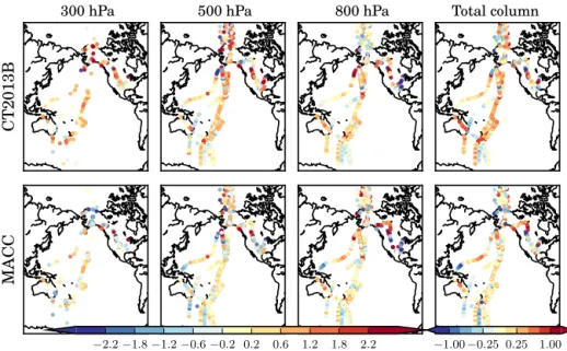
Figure 2 shows an overview of model–HIPPO differences at three pressure levels as well as XCO2, the total column
av-erage. For the differences in XCO2, the respective model has
been used to extend the HIPPO profiles from its highest alti-tude to the top of atmosphere; hence, part of the smaller dif-ferences observed in XCO2comparisons can stem from the
fact that the model contributes slightly to the HIPPO-based XCO2 as well, though the tropospheric variability should
dominate. As can be seen in the left panels, not all HIPPO profiles extend up to 300 hPa.
Unsurprisingly, model-data mismatches at individual lev-els are substantially higher than in the total column, about a factor of 2. Many differences are not consistent between the two models, for example during HIPPO 4N, extending from West Papua northwards. In MACC, there is first a substantial underestimation throughout the profile and then an overesti-mation further north. In CT2013B, no obvious discrepancies can be observed. In other areas, such as the same HIPPO 4N path south of Alaska, MACC appears rather consistent but CT2013B is much higher at 800 hPa but much lower at 500 hPa, with a slight underestimation in the total column.
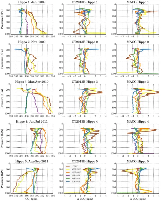
Figure 3 provides an in-depth review of HIPPO – model comparisons for profiles averaged by latitudinal bands and campaign. In most cases, profiles agree to within 1 ppm with a few notable exceptions, mostly at higher latitudes during the drawdown or respiration maximum in HIPPO 5 and 3, respectively. These are typically associated with steep verti-cal gradients around 300 hPa, both in HIPPO 5 and 3, albeit with different signs. In most other cases, the differences even in the profiles are usually below 1 ppm, underlining the
strin-CT2013B
300 hPa 500 hPa 800 hPa Total column
MACC
−2.2 −1.8 −1.2 −0.6 −0.2 0.2 0.6 1.2 1.8 2.2 ∆CO2(ppm), model-HIPPO
−1.00 −0.25 0.25 1.00 ∆XCO2(ppm), model-HIPPO
Figure 2. Top row, from left to right: CT2013B–HIPPO differences at 300, 500, 800 hPa, and column-averaged mixing ratio of CO2. Bottom
row: as for the top row but for the MACC model. Note the change in color scale between layer and total column differences. All HIPPO campaigns are included.
gent accuracy requirements for space-based CO2
measure-ments, as atmospheric models optimized with respect to the ground-based network already model oceanic background concentrations fairly well. However, the caveat is that these ground-based stations are also located in remote regions, ide-ally not affected by local sources. On smaller spatial scales near sources, space-based measurements can provide valu-able information even in the presence of potential large-scale biases.
Figure 4 shows an in-depth comparison of the largest model–HIPPO discrepancies, namely the high latitude pro-files during HIPPO 3 and 5. As one can see in the left panels, the seasonal cycles in the mid-troposphere and at 200 hPa can be opposite, with large CO2values in the upper atmosphere
during the largest CO2drawdown and vice versa during the
peak of respiration. Model–HIPPO mismatches are most ob-vious and similar between models in HIPPO 3 (March/April 2010), with differences reaching up to 4 ppm at 300 hPa. This is consistent with a comparison against the GEOS-Chem model by Deng et al. (2015), who studied the impact of dis-crepancies in stratosphere–troposphere exchange on inferred sources and sinks of CO2. In HIPPO 5, at the end of the
growing season, the situation is reversed as the profile slopes change sign after the large CO2uptake during summer. For
HIPPO 5, the deviations for CT2013B are somewhat smaller but it can be seen that most models suffer from these po-tential biases if large vertical gradients exist. Overall, both CT2013B as well as MACC show a good agreement with HIPPO over the oceans.
4 Comparisons of column-averaged mixing ratios Here, we look at XCO2, derived using absorption
troscopy of reflected sunlight recorded by near-infrared spec-trometers such as SCIAMACHY, GOSAT, or Orbiting Car-bon Observatory-2 (OCO-2). In this paper, we only used data from GOSAT as it is the only instrument having sampled in Glint mode during the HIPPO investigation. SCIAMACHY data have not been used as it has no dedicated glint mode and the SCIAMACHY products (e.g., Reuter et al., 2011) are limited to retrievals over land.
For the comparison of column-averaged mixing ratios, we need to extend the HIPPO profiles to the top of atmo-sphere. For this, we use the respective atmospheric model for comparison. In addition, we computed the average HIPPO XCO2for each campaign using all the data and subsequently
removed it from individual measurements, both from the HIPPO, model and satellite data. This ensures that observed correlations are driven predominantly by spatial gradients within a campaign period and not by the secular trend. For the HIPPO comparison against GOSAT data, we take the in-strument sensitivity into account by applying the averaging kernel to the difference of the true profile (using the model-extended HIPPO data set as truth) and the respective a priori profile. We perform this correction using both model exten-sions independently and then use the average of the two. 4.1 Atmospheric models
In terms of XCO2, both atmospheric models used here
com-pare well against HIPPO, as can be seen in Figs. 5 and 6. Even after normalization with the campaign average, the
cor-380 382 384 386 388 390 392 394 396 0 200 400 600 800 1000 Pr es su re [h Pa ] Hippo 1; Jan. 2009 −4 −3 −2 −1 0 1 2 3 4 0 200 400 600 800 1000 CT2013B-Hippo 1 −4 −3 −2 −1 0 1 2 3 4 0 200 400 600 800 1000 MACC-Hippo 1 380 382 384 386 388 390 392 394 396 0 200 400 600 800 1000 Pr es su re [h Pa ] Hippo 2; Nov. 2009 −4 −3 −2 −1 0 1 2 3 4 0 200 400 600 800 1000 CT2013B-Hippo 2 −4 −3 −2 −1 0 1 2 3 4 0 200 400 600 800 1000 MACC-Hippo 2 380 382 384 386 388 390 392 394 396 0 200 400 600 800 1000 Pr es su re [h Pa ] Hippo 3; Mar/Apr 2010 −4 −3 −2 −1 0 1 2 3 4 0 200 400 600 800 1000 CT2013B-Hippo 3 −4 −3 −2 −1 0 1 2 3 4 0 200 400 600 800 1000 MACC-Hippo 3 380 382 384 386 388 390 392 394 396 0 200 400 600 800 1000 Pr es su re [h Pa ] Hippo 4; Jun/Jul 2011 −4 −3 −2 −1 0 1 2 3 4 0 200 400 600 800 1000 CT2013B-Hippo 4 −4 −3 −2 −1 0 1 2 3 4 0 200 400 600 800 1000 MACC-Hippo 4 380 382 384 386 388 390 392 394 396 CO2(ppm) 0 200 400 600 800 1000 Pr es su re [h Pa ] Hippo 5; Aug/Sep 2011 −4 −3 −2 −1 0 1 2 3 4 ∆CO2(ppm) 0 200 400 600 800 1000 CT2013B-Hippo 5 >70N 45N-70N 15N-45N 15S-15N 45S-15S 70S-45S −4 −3 −2 −1 0 1 2 3 4 ∆CO2(ppm) 0 200 400 600 800 1000 MACC-Hippo 5
Figure 3. Summary of averaged CO2 HIPPO profiles in ppm (left column) and model–HIPPO differences (middle and right column), separated by latitudinal bands (color coded) and HIPPO campaign (separate rows).
relation coefficients and slopes are r2=0.93 (slope = 0.95) for CT2013B and r2=0.95 (slope = 1.00) for MACC. South of 20◦N, almost all data points lie within ±1 ppm with some outliers of up to 3 ppm at higher latitudes, mostly over the continents (see Fig. 2).
These numbers should not be used to compare the mod-els against each other because, as evident in Fig. 2, there are regions where either one or the other model is in bet-ter agreement with HIPPO. In conclusion, one can state that most model mismatches are below 1 ppm in remote areas, such as the oceans, and can reach 2–3 ppm over the conti-nents with potentially higher values in under-sampled areas with high CO2uptake such as the US corn belt. In addition,
it should be mentioned that both models ingest a multitude
of CO2measurements at US ground-based stations and areas
further away might be less well modeled. However, the excel-lent agreement provides a benchmark against which satellite retrievals have to be measured.
4.2 GOSAT
The comparison of GOSAT satellite data against HIPPO is somewhat more complicated because there is not necessarily a matching GOSAT measurement with each HIPPO profile. For coincidence criteria, we follow exactly Kulawik et al. (2015), based on the dynamic co-location criteria detailed in Wunch et al. (2011) and Keppel-Aleks et al. (2011, 2012). In addition, we require that the difference of CT2013B sampled at the HIPPO and the actual GOSAT location is less than
375 380 385 390 395 0 200 400 600 800 1000 Pr es su re [h Pa ] Hippo 5 MACC CT2013B HIPPO 375 380 385 390 395 CO2[ppm] 0 200 400 600 800 1000 Pr es su re [h Pa ] Hippo 3 −8 −6 −4 −2 0 2 4 6 8 0 200 400 600 800 1000 pressure [hP a] Hippo 5 MACC-HIPPO CT2013B-HIPPO −8 −6 −4 −2 0 2 4 6 8 ∆CO2[ppm] 0 200 400 600 800 1000 pressure [hP a] Hippo 3
Figure 4. Averaged HIPPO and matched model profiles for latitudes > 70◦N during HIPPO 3 and 5, respectively. The left panels show model and HIPPO profiles and the right panels show model–HIPPO average differences as well as their range in the thinner and somewhat transparent colors. −4 −2 0 2 4 HIPPO XCO2(ppm) −4 −2 0 2 4 CT2013B XCO 2 (ppm) Slope= 0.95 r2= 0.93 HIPPO 1S HIPPO 1N HIPPO 2S HIPPO 2N HIPPO 3S HIPPO 3N HIPPO 4S HIPPO 4N HIPPO 5S HIPPO 5N −80 −60 −40 −20 0 20 40 60 80 100 Latitude −3 −2 −1 0 1 2 3 ∆ XCO 2 (ppm) Mean= 0.10 SD= 0.51
Figure 5. Left: scatter plot of normalized (with campaign aver-age) XCO2 computed from individual HIPPO profiles (x axis)
against corresponding CT2013B data. Right: difference plot of XCO2against latitude. Campaigns as well as north and southbound
tracks are color coded.
0.5 ppm, thereby bounding the error introduced by the spa-tial mismatch between HIPPO and respective GOSAT sound-ings. For each match, the standard error in the GOSAT XCO2
average is computed using the standard deviation of all cor-responding GOSAT co-locations divided by the square root of the number of co-locations.
For the GOSAT comparison, we require at least five co-located GOSAT measurement per HIPPO profile, all of which are subsequently averaged before comparison against HIPPO. HIPPO XCO2is computed as the average of MACC
−4 −2 0 2 4 HIPPO XCO2(ppm) −4 −2 0 2 4 MACC XCO 2 (ppm) Slope= 1.00 r2= 0.95 HIPPO 1S HIPPO 1N HIPPO 2S HIPPO 2N HIPPO 3S HIPPO 3N HIPPO 4S HIPPO 4N HIPPO 5S HIPPO 5N −80 −60 −40 −20 0 20 40 60 80 100 Latitude −3 −2 −1 0 1 2 3 ∆ XCO 2 (ppm) Mean= 0.06 SD= 0.43
Figure 6. Left: scatter plot of normalized (with campaign average) XCO2computed from individual HIPPO profiles (x axis) against
corresponding MACC data. Right: difference plot of XCO2against
latitude. Campaigns as well as north and southbound tracks are color coded.
and CT2013B extended HIPPO profiles with the difference between the two used as uncertainty range for HIPPO.
In Fig. 7, the scatter plot of HIPPO vs. GOSAT is depicted. It is obvious that the data density is far lower than that of the models because (a) HIPPO 1 is not overlapping in time and (b) only a subset of HIPPO profiles is matched with enough co-located GOSAT soundings. This gives rise to a reduced dynamic range in XCO2, from about a −1.5 to 3 ppm
differ-ence to the campaign average. However, both slope and r2 are also in excellent agreement with HIPPO and only very few points are exceeding a 1 ppm difference. Those that are
−3 −2 −1 0 1 2 3 HIPPO XCO2(ppm) −3 −2 −1 0 1 2 3 GOSA T XCO 2 (ppm) Slope= 0.99 r2= 0.85 HIPPO 2S HIPPO 2N HIPPO 3S HIPPO 3N HIPPO 4S HIPPO 4N HIPPO 5S HIPPO 5N −60 −40 −20 0 20 40 60 Latitude −2.0 −1.5 −1.0 −0.5 0.0 0.5 1.0 1.5 2.0 ∆ XCO 2 (ppm) Mean= -0.06 SD= 0.45 CT2013B-HIPPO MACC-HIPPO
Figure 7. Left: scatter plot of normalized (with campaign average) XCO2computed from individual HIPPO profiles (x axis) against
corresponding GOSAT data. Right: difference plot of XCO2against
latitude. Campaigns as well as north and southbound tracks are color coded. For comparison, the right panel also shows the model– HIPPO differences in smaller symbols without error bar (MACC as “+”, CT2013B as “x”).
< −1 ppm are also associated with larger uncertainties in-duced by model extrapolation, as seen in the larger error bars for HIPPO in the left panel (in particular for HIPPO 2S). The right panel shows the discrepancies for the models as well, just for the subset that could be compared against GOSAT and using the model sampled at the GOSAT locations.
One can see that it is hard to make a clear statement on whether GOSAT or the models compare better with HIPPO. Figure 8 shows this comparison in more detail, plotting model–HIPPO differences on the x axis and GOSAT–model differences on the y axis. As before, the error bar for GOSAT is derived as the standard error in the mean and the model er-ror bar by using the variability of HIPPO XCO2using the two
different models to extrapolate to the top-of-atmosphere (and the average of the two is defined as HIPPO XCO2. The center
box spans a range from −0.5 to 0.5 ppm, a strict requirement for systematic biases (GHG-CCI, 2014). The green and red shaded areas indicated regions where either the GOSAT data meet the 0.5 ppm requirement but the models do not (green) or vice versa (red). Given the small amount of samples, it is premature to draw strong conclusions but it appears that somewhat more points lie in the green area. It also has to be pointed out that pure measurement unsystematic noise also contributes to the scatter in GOSAT.
For MACC, there is even a noticeable correlation between MACC–HIPPO and GOSAT–HIPPO with an r2of 0.26. This can hint at either small-scale features caught by HIPPO and missed by both GOSAT and models or small systematic vari-ability between the exact HIPPO and GOSAT co-location. Most of the samples causing the high r2are located in the lower left quadrant, underestimated by GOSAT as well as both models and apparently all within HIPPO 2S, located be-tween 40 and 20◦S. −1.5−1.0−0.5 0.0 0.5 1.0 1.5 CT2013B-HIPPO XCO2(ppm) −1.5 −1.0 −0.5 0.0 0.5 1.0 1.5 Slope= 0.33 r2= 0.10 −1.5−1.0−0.5 0.0 0.5 1.0 1.5 MACC-HIPPO XCO2(ppm) −1.5 −1.0 −0.5 0.0 0.5 1.0 1.5 GOSA T-HIPPO XCO 2 (ppm) Slope= 0.53 r2= 0.26
Figure 8. Left: scatter plot of 1 XCO2 (CT-HIPPO) against 1
XCO2 (GOSAT–HIPPO), using just the GOSAT subsets. Right:
same as left but using MACC instead of CT2013B. The inner box represents the area where both model and GOSAT are within 0.5 ppm compared to HIPPO, which corresponds to the very strin-gent accuracy requirement. The green and red shaded areas corre-spond to regions where the satellite deviates less than the models and is within 0.5 ppm (green) as well as where the models deviate less than GOSAT (red). The white cells on the outer edges indicate areas where both deviate more than 0.5 ppm overall.
200 300 400 500 600 700 800 900 1000 Pr es su re (h P a )
HIPPO campaign No. 2 southbound
−50 −45 −40 −35 −30 −25 −20 −15 −10 Latitude 200 300 400 500 600 700 800 900 1000 Pr es su re (h P a ) −2.0 −1.6 −1.2 −0.8 −0.4 0.0 0.4 0.8 1.2 1.6 2.0 ∆ X CO 2 [ppm] 32 40 48 56 64 72 80 88 96 HIPPO CO [ppb]
Figure 9. Top: MACC–HIPPO CO2differences (ppm) as a function of latitude and pressure level during the HIPPO 2 southbound cam-paign, recorded on 10–11 November 2009. Bottom: corresponding HIPPO CO measurements (ppb).
Figure 9 depicts the HIPPO 2S campaign in more detail, showing the exact flight patterns and the differences with respect to MACC (MACC–HIPPO) at each measurement point (upper panel). For the sake of simplicity, we only show MACC here. The measured CO concentrations are shown in
the lower panel. There is enhanced carbon monoxide (CO) at higher altitudes, indicating long-range transport of biomass burning at the time of overflight, which can explain the ap-parent model–HIPPO mismatch. The features span several degrees of latitude, excluding coarse model resolution as a reason for missing the plume. Thus, we hypothesize that the mismatch is caused by either underestimated CO emissions from the Global Fire Emissions Database (GFED, Randerson et al., 2013; which is used by both models) or transport er-rors in the models. For GOSAT, the mismatch is most likely caused by too lenient coincidence criteria, missing most of the biomass burning plume.
Overall, it can be concluded that GOSAT measurements can provide valuable and accurate information on the global CO2distribution and meets the 0.5 ppm bias criterion in most
cases over the ocean. However, small sampling sizes pre-cludes an in-depth analysis of potential large-scale biases in the data sets. In the future, OCO-2 with its much higher sam-pling density will help to disentangle measurement and mod-eling bias and guide inversion studies.
5 Comparisons of mid- to upper-tropospheric CO2
5.1 TES (∼ 510 hPa)
For the comparison with TES, we use the 510 hPa retrieval layer and apply averaging kernel corrections using model-extended HIPPO data as truth, using both models indepen-dently and averaging results after averaging kernel correc-tion. Coincidence criteria are identical to the GOSAT analy-sis but we require at least 20 valid TES soundings per HIPPO profile to reduce measurement noise. Similar to before, the TES error bars are empirically derived using the standard de-viation of the co-located soundings.
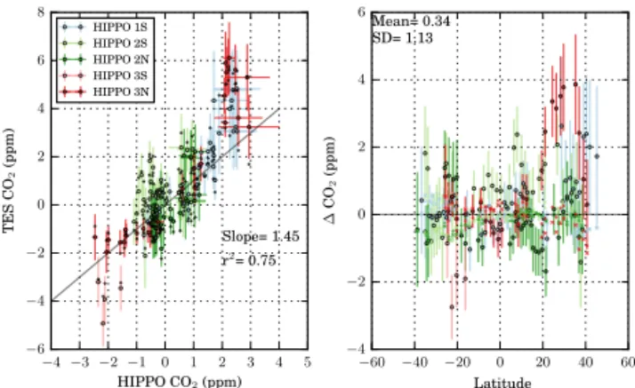
Figure 10 shows the comparison of TES against HIPPO in the same way it was for GOSAT. The correlation (r2) is somewhat lower than for GOSAT but still very significant. Some differences exceed 2 ppm, albeit with a relatively high standard error, i.e., barely significant at the 2-σ level (see right panel, error bars indicate 1-σ ).
Given the larger standard error in TES data, differences may be purely noise driven and not necessarily a hint at large-scale biases even though the clustering of positive anoma-lies, in particular in HIPPO 3 at higher latitudes, is apparent. As evident from Fig. 3, there are stronger vertical gradients at 15–45◦N during HIPPO3 because they are close to the peak CO2 value caused by wintertime respiration. This can
cause potential mismatches as gradients can be strong and co-location criteria might have to be more strict. In addition, the HIPPO profiles are extended by models to the top of at-mosphere and are thus not entirely model independent.
−4 −3 −2 −1 0 1 2 3 4 5 HIPPO CO2(ppm) −6 −4 −2 0 2 4 6 8 TES CO 2 (ppm) Slope= 1.45 r2= 0.75 HIPPO 1S HIPPO 2S HIPPO 2N HIPPO 3S HIPPO 3N −60 −40 −20 0 20 40 60 Latitude −4 −2 0 2 4 6 ∆ CO 2 (ppm) Mean= 0.34 SD= 1.13
Figure 10. Left: scatter plot of normalized (with campaign average) CO2from individual HIPPO profiles (x axis) against corresponding
TES data. Right: difference plot of CO2against latitude. Campaigns
as well as north and southbound tracks are color coded, model– HIPPO differences are plotted as well. Please refer to Fig. 7 for a detailed legend. −6 −4 −2 0 2 4 6 HIPPO CO2(ppm) −6 −4 −2 0 2 4 6 AIRS CO 2 (ppm) Slope= 0.66 r2= 0.37 −60 −40 −20 0 20 40 60 Latitude −4 −2 0 2 4 6 ∆ CO 2 (ppm) Mean= 1.11 SD= 1.46
Figure 11. Left: scatter plot of normalized (with campaign aver-age) CO2from individual HIPPO profiles (x axis) against
corre-sponding AIRS data. Right: difference plot of CO2against latitude.
Campaigns as well as north and southbound tracks are color coded, model–HIPPO differences are plotted as well. Please refer to Fig. 7 for a detailed legend.
5.2 AIRS (∼ 300 hPa)
For the comparison with AIRS (Fig. 11), the sensitivity max-imum varies around 300 hPa and we apply the averaging ker-nels similar to TES. Owing to the large data density and high single measurement noise of AIRS, we use a minimum of 50 co-locations for a comparison, still leaving many more data points than for the GOSAT and TES comparison. As coinci-dence criteria, we use data within 5◦ latitude and longitude and 24 h time difference.
Even though the correlations are significant, a bias depen-dence on latitude can be observed, which hampers incorpo-ration of AIRS data into flux inversions. The reason for these biases is currently unknown but may be related to changes in peak sensitivity altitude as a function of latitude. A full
Table 1. Summary of all HIPPO comparisons. No. of profiles shows how many HIPPO profiles were used for the comparison. Correlation coefficients, fitted slope, mean difference µ, and standard deviation σ of the difference compared to HIPPO of all comparisons are computed using measurements normalized by the respective campaign average. For comparison, σ of model–HIPPO for the satellite co-locations and respective sensitivity are provided as well.
No. profiles r2 slope µ(ppm) σ(ppm) σCT σMACC
GOSAT 94 0.85 0.99 −0.06 0.45 0.42 0.36 TES 135 0.75 1.45 0.34 1.13 0.36 0.3 AIRS 200 0.37 0.66 1.11 1.46 0.63 0.47 CT2013B 676 0.93 0.95 0.10 0.51 N/A N/A MACC 674 0.95 1.00 0.06 0.43 N/A N/A
characterization of averaging kernels per sounding would alleviate these concerns. Given the observed larger model– HIPPO CO2 differences at higher altitudes, a fully
charac-terized AIRS CO2product could be worthwhile for the flux
community. However, requirements for systematic biases in partial columns are even stricter than for the total column (Chevallier, 2015).
6 Conclusions
In this study, we compared atmospheric models as well as satellite data of CO2 against HIPPO profiles. Table 1
pro-vides a high-level overview of the derived statistics. Both atmospheric models compare very similarly, both showing a very high correlation with respect to HIPPO, even when subtracting the campaign average XCO2, as is done
through-out all comparisons. The largest discrepancies are found near 300 hPa at higher latitudes during peak wintertime CO2
ac-cumulation as well as the summer uptake period. These may be related to steep vertical gradients poorly resolved by the models. In addition, a biomass burning event in the South-ern Hemisphere seems to have been underestimated by the models, causing discrepancies of around 1 ppm.
For GOSAT comparisons, results are comparable to those with models but the sample size is much smaller. OCO-2 could largely improve on GOSAT’s data density over the oceans but did not overlap with the HIPPO measurement campaign period. The new Atmospheric Tomography Mis-sion (ATom), selected as one of NASA’s Earth Venture air-borne missions, will potentially allow for similar compar-isons to OCO-2 in the future and should provide enough data to draw more robust conclusions than using GOSAT.
In general, GOSAT compares very well to HIPPO, fol-lowed by TES and AIRS. For TES, most deviations can be explained by pure measurement noise but AIRS appears to exhibit some latitudinal biases that would need to be ac-counted for if used for source-inversion studies. On the other hand, systematic model transport errors that can affect source inversions (Deng et al., 2015) were confirmed here for both atmospheric models used. Despite initial skepticism towards using remotely sensed CO2data for global carbon-cycle
in-version, we are now reaching a state where potential sys-tematic errors in both remote sensing as well as atmospheric modeling can play an equally crucial part. Innovative meth-ods to characterize and ideally minimize both of these error sources will be needed in the future. One option is to ap-ply flux inversion schemes that co-retrieve systematic biases alongside fluxes, such as in Bergamaschi et al. (2007), using prior knowledge on potential physical insight into systematic biases, such as aerosol interference, land/ocean biases or air mass factors.
7 Data availability
CarbonTracker CT2013B data are available at http:// carbontracker.noaa.gov. MACC data are available at https: //atmosphere.copernicus.eu. TES data are available at http: //tes.jpl.nasa.gov/data/. HIPPO data are available at http: //hippo.ornl.gov. AIRS data are available at http://disc.sci. gsfc.nasa.gov/uui/datasets?keywords=AIRS. GOSAT data processed by NASA/JPL as well as a general CO2repository
are available at http://co2.jpl.nasa.gov.
Acknowledgements. Funded by NASA Roses ESDR-ERR 10/10-ESDRERR10-0031, “Estimation of biases and errors of CO2
satellite observations from AIRS, GOSAT, SCIAMACHY, TES, and OCO-2”. We thank the entire HIPPO team for making these measurements possible and the NIES and JAXA GOSAT teams for designing and operating the GOSAT mission and generously sharing L1 data with the ACOS project. Andy Jacobson (NOAA ESRL, Boulder, Colorado) provided CarbonTracker CT2013B results and advised in data usage and interpretation.
References
Basu, S., Krol, M., Butz, A., Clerbaux, C., Sawa, Y., Machida, T., Matsueda, H., Frankenberg, C., Hasekamp, O., and Aben, I.: The seasonal variation of the CO2flux over Tropical Asia estimated
from GOSAT, CONTRAIL, and IASI, Geophys. Res. Lett., 41, 1809–1815, 2014.
Bergamaschi, P., Frankenberg, C., Meirink, J. F., Krol, M., Dentener, F., Wagner, T., Platt, U., Kaplan, J. O., Körner, S., Heimann, M., Dlugokencky, E. J., and Goede, A.: Satellite chartography of atmospheric methane from SCIA-MACHY on board ENVISAT: 2. Evaluation based on inverse model simulations, J. Geophys. Res.-Atmos., 112, D02304, doi:10.1029/2006JD007268, 2007.
Chahine, M., Barnet, C., Olsen, E. T., Chen, L., and Maddy, E.: On the determination of atmospheric minor gases by the method of vanishing partial derivatives with application to CO2, Geophys.
Res. Lett., 32, L22803, doi:10.1029/2005GL024165, 2005. Chevallier, F.: On the statistical optimality of CO2 atmospheric
inversions assimilating CO2 column retrievals, Atmos. Chem.
Phys., 15, 11133–11145, doi:10.5194/acp-15-11133-2015, 2015. Deng, F., Jones, D. B. A., Walker, T. W., Keller, M., Bowman, K. W., Henze, D. K., Nassar, R., Kort, E. A., Wofsy, S. C., Walker, K. A., Bourassa, A. E., and Degenstein, D. A.: Sensitivity anal-ysis of the potential impact of discrepancies in stratosphere-troposphere exchange on inferred sources and sinks of CO2,
Atmos. Chem. Phys., 15, 11773–11788, doi:10.5194/acp-15-11773-2015, 2015.
GHG-CCI: User Requirements Document for the GHG-CCI project of ESA’s Climate Change Initiative, 38 pp., version 2, 28 Aug. 2014, Tech. rep., ESA, available at: http://www.esa-ghg-cci.org/ ?q=webfm_send/173, 2014.
Guerlet, S., Basu, S., Butz, A., Krol, M., Hahne, P., Houweling, S., Hasekamp, O., and Aben, I.: Reduced carbon uptake during the 2010 Northern Hemisphere summer from GOSAT, Geophys. Res. Lett., 40, 2378–2383, 2013.
Hamazaki, T., Kaneko, Y., Kuze, A., and Kondo, K.: Fourier transform spectrometer for greenhouse gases observing satellite (GOSAT), in: Proceedings of SPIE, vol. 5659, p. 73, 2005. Hourdin, F. and Armengaud, A.: The use of finite-volume methods
for atmospheric advection of trace species – Part I: Test of var-ious formulations in a general circulation model, Mon. Weather Rev., 127, 822–837, 1999.
Hourdin, F., Musat, I., Bony, S., Braconnot, P., Codron, F., Dufresne, J.-L., Fairhead, L., Filiberti, M.-A., Friedlingstein, P., Grandpeix, J.-Y., Krinner, G., LeVan, P., Li, Z.-X., and Lott, F.: The LMDZ4 general circulation model: climate performance and sensitivity to parametrized physics with emphasis on tropical convection, Clim. Dynam., 27, 787–813, doi:10.1007/s00382-006-0158-0, 2006.
Houweling, S., Baker, D., Basu, S., Boesch, H., Butz, A., Cheval-lier, F., Deng, F., Dlugokencky, E. J., Feng, L., Ganshin, A., Hasekamp, O., Jones, D., Maksyutov, S., Marshall, J., Oda, T., O’Dell, C. W., Oshchepkov, S., Palmer, P. I., Peylin, P., Poussi, Z., Reum, F., Takagi, H., Yoshida, Y., and Zhuravlev, R.: An in-tercomparison of inverse models for estimating sources and sinks of CO2using GOSAT measurements, J. Geophys. Res.-Atmos., 120, 5253–5266, doi:10.1002/2014JD022962, 2015.
Keppel-Aleks, G., Wennberg, P. O., and Schneider, T.: Sources of variations in total column carbon dioxide, Atmos. Chem. Phys., 11, 3581–3593, doi:10.5194/acp-11-3581-2011, 2011.
Keppel-Aleks, G., Wennberg, P. O., Washenfelder, R. A., Wunch, D., Schneider, T., Toon, G. C., Andres, R. J., Blavier, J.-F., Con-nor, B., Davis, K. J., Desai, A. R., Messerschmidt, J., Notholt, J., Roehl, C. M., Sherlock, V., Stephens, B. B., Vay, S. A., and Wofsy, S. C.: The imprint of surface fluxes and transport on vari-ations in total column carbon dioxide, Biogeosciences, 9, 875– 891, doi:10.5194/bg-9-875-2012, 2012.
Krol, M., Houweling, S., Bregman, B., van den Broek, M., Segers, A., van Velthoven, P., Peters, W., Dentener, F., and Bergamaschi, P.: The two-way nested global chemistry-transport zoom model TM5: algorithm and applications, Atmos. Chem. Phys., 5, 417– 432, doi:10.5194/acp-5-417-2005, 2005.
Kulawik, S. S., Worden, J. R., Wofsy, S. C., Biraud, S. C., Nassar, R., Jones, D. B. A., Olsen, E. T., Jimenez, R., Park, S., Santoni, G. W., Daube, B. C., Pittman, J. V., Stephens, B. B., Kort, E. A., Osterman, G. B., and TES team: Comparison of improved Aura Tropospheric Emission Spectrometer CO2with HIPPO and SGP
aircraft profile measurements, Atmos. Chem. Phys., 13, 3205– 3225, doi:10.5194/acp-13-3205-2013, 2013.
Kulawik, S., Wunch, D., O’Dell, C., Frankenberg, C., Reuter, M., Oda, T., Chevallier, F., Sherlock, V., Buchwitz, M., Osterman, G., Miller, C. E., Wennberg, P. O., Griffith, D., Morino, I., Dubey, M. K., Deutscher, N. M., Notholt, J., Hase, F., Warneke, T., Sussmann, R., Robinson, J., Strong, K., Schneider, M., De Maz-ière, M., Shiomi, K., Feist, D. G., Iraci, L. T., and Wolf, J.: Consistent evaluation of ACOS-GOSAT, BESD-SCIAMACHY, CarbonTracker, and MACC through comparisons to TCCON, Atmos. Meas. Tech., 9, 683–709, doi:10.5194/amt-9-683-2016, 2016.
Kuze, A., Suto, H., Nakajima, M., and Hamazaki, T.: Thermal and near infrared sensor for carbon observation Fourier-transform spectrometer on the Greenhouse Gases Observing Satellite for greenhouse gases monitoring, Appl. Opt., 48, 6716–6733, 2009. Lindqvist, H., O’Dell, C. W., Basu, S., Boesch, H., Chevallier, F., Deutscher, N., Feng, L., Fisher, B., Hase, F., Inoue, M., Kivi, R., Morino, I., Palmer, P. I., Parker, R., Schneider, M., Sussmann, R., and Yoshida, Y.: Does GOSAT capture the true seasonal cy-cle of carbon dioxide?, Atmos. Chem. Phys., 15, 13023–13040, doi:10.5194/acp-15-13023-2015, 2015.
Miller, C. E., Crisp, D., DeCola, P. L., Olsen, S. C., Randerson, J. T., Michalak, A. M., Alkhaled, A., Rayner, P., Jacob, D. J., Suntharalingam, P., Jones, D. B. A., Denning, A. S., Nicholls, M. E., Doney, S. C., Pawson, S., Boesch, H., Connor, B. J., Fung, I. Y., O’Brien, D., Salawitch, R. J., Sander, S. P., Sen, B., Tans, P., Toon, G. C., Wennberg, P. O., Wofsy, S. C., Yung, Y. L., and Law, R. M.: Precision requirements for space-based data, J. Geophys. Res.-Atmos., 112, D10314, doi:10.1029/2006JD007659, , 2007. O’Dell, C. W., Connor, B., Bösch, H., O’Brien, D., Frankenberg, C., Castano, R., Christi, M., Eldering, D., Fisher, B., Gunson, M., McDuffie, J., Miller, C. E., Natraj, V., Oyafuso, F., Polonsky, I., Smyth, M., Taylor, T., Toon, G. C., Wennberg, P. O., and Wunch, D.: The ACOS CO2retrieval algorithm – Part 1: Description and
validation against synthetic observations, Atmos. Meas. Tech., 5, 99–121, doi:10.5194/amt-5-99-2012, 2012.
Olsen, E. T. and Licata, S. J.: AIRS Version 5 Release Tropospheric CO2Products, Tech. rep., Jet Propulsion Laboratory, California
Institute of Technology, available at: http://disc.sci.gsfc.nasa. gov/AIRS/documentation/v5_docs/AIRS%_V5_Release_User_ Docs/AIRS-V5-Tropospheric-CO2-Products.pdf, 2014. Peters, W., Jacobson, A. R., Sweeney, C., Andrews, A. E.,
Con-way, T. J., Masarie, K., Miller, J. B., Bruhwiler, L. M. P., brielle Petron, G., Hirsch, A. I., Worthy, D. E. J., van der Werf, G. R., Randerson, J. T., Wennberg, P. O., Krol, M. C., and Tans, P. P.: An atmospheric perspective on North American carbon dioxide exchange: CarbonTracker, P. Natl. Acad. Sci. USA, 104, 18 925– 18 930, doi:10.1073/pnas.0708986104, 2007.
Randerson, J., van der Werf, G., Giglio, L., Col-latz, G., and Kasibhatla, P.: Global Fire Emissions Database, Version 3 (GFEDv3.1), Tech. rep., ORNL, doi:10.3334/ORNLDAAC/1191, 2013.
Reuter, M., Bovensmann, H., Buchwitz, M., Burrows, J., Con-nor, B., Deutscher, N. M., Griffith, D., Heymann, J., Keppel-Aleks, G., Messerschmidt, J., Notholt, J., Petri, C., Robin-son, J., Schneising, O., Sherlock, V., Velazco, V., Warneke, T., Wennberg, P. O., and Wunch, D.: Retrieval of atmo-spheric CO2with enhanced accuracy and precision from
SCIA-MACHY: Validation with FTS measurements and comparison with model results, J. Geophys. Res-Atmos., 116, D04301, doi:10.1029/2010JD015047, 2011.
Schneising, O., Reuter, M., Buchwitz, M., Heymann, J., Bovens-mann, H., and Burrows, J. P.: Terrestrial carbon sink observed from space: variation of growth rates and seasonal cycle am-plitudes in response to interannual surface temperature variabil-ity, Atmos. Chem. Phys., 14, 133–141, doi:10.5194/acp-14-133-2014, 2014.
Stephens, B. B., Gurney, K. R., Tans, P. P., Sweeney, C., Peters, W., Bruhwiler, L., Ciais, P., Ramonet, M., Bousquet, P., Nakazawa, T., Aoki, S., Machida, T., Inoue, G., Vinnichenko, N., Lloyd, J., Jordan, A., Heimann, M., Shibistova, O., Langenfelds, R. L., Steele, L. P., Francey, R. J., and Denning, A. S.: Weak northern and strong tropical land carbon uptake from vertical profiles of atmospheric CO2, Science, 316, 1732–1735, 2007.
Wofsy, S. C.: HIAPER Pole-to-Pole Observations (HIPPO): fine-grained, global-scale measurements of climatically important at-mospheric gases and aerosols, Philos. T. R. Soc. A, 369, 2073– 2086, doi:10.1098/rsta.2010.0313, 2011.
Wunch, D., Wennberg, P. O., Toon, G. C., Connor, B. J., Fisher, B., Osterman, G. B., Frankenberg, C., Mandrake, L., O’Dell, C., Ahonen, P., Biraud, S. C., Castano, R., Cressie, N., Crisp, D., Deutscher, N. M., Eldering, A., Fisher, M. L., Griffith, D. W. T., Gunson, M., Heikkinen, P., Keppel-Aleks, G., Kyrö, E., Lindenmaier, R., Macatangay, R., Mendonca, J., Messerschmidt, J., Miller, C. E., Morino, I., Notholt, J., Oyafuso, F. A., Ret-tinger, M., Robinson, J., Roehl, C. M., Salawitch, R. J., Sher-lock, V., Strong, K., Sussmann, R., Tanaka, T., Thompson, D. R., Uchino, O., Warneke, T., and Wofsy, S. C.: A method for eval-uating bias in global measurements of CO2total columns from
space, Atmos. Chem. Phys., 11, 12317–12337, doi:10.5194/acp-11-12317-2011, 2011.


![[PDF] Introduction à HTML 5 ressource de formation approfondie | Cours INFORMATIQUE](data:image/gif;base64,R0lGODlhAQABAIAAAP///wAAACH5BAEAAAAALAAAAAABAAEAAAICRAEAOw==)