HAL Id: hal-03158662
https://hal.archives-ouvertes.fr/hal-03158662
Submitted on 4 Mar 2021
HAL is a multi-disciplinary open access
archive for the deposit and dissemination of
sci-entific research documents, whether they are
pub-lished or not. The documents may come from
teaching and research institutions in France or
abroad, or from public or private research centers.
L’archive ouverte pluridisciplinaire HAL, est
destinée au dépôt et à la diffusion de documents
scientifiques de niveau recherche, publiés ou non,
émanant des établissements d’enseignement et de
recherche français ou étrangers, des laboratoires
publics ou privés.
assess the potential of spaceborne CO2 measurements
for the monitoring of anthropogenic emissions
Diego Santaren, Grégoire Broquet, François-Marie Bréon, Frederic Chevallier,
Denis Siméoni, Bo Zheng, Philippe Ciais
To cite this version:
Diego Santaren, Grégoire Broquet, François-Marie Bréon, Frederic Chevallier, Denis Siméoni, et al..
A local- to national-scale inverse modeling system to assess the potential of spaceborne CO2
mea-surements for the monitoring of anthropogenic emissions. Atmospheric Measurement Techniques,
European Geosciences Union, 2021, 14 (1), pp.403-433. �10.5194/amt-14-403-2021�. �hal-03158662�
https://doi.org/10.5194/amt-14-403-2021 © Author(s) 2021. This work is distributed under the Creative Commons Attribution 4.0 License.
A local- to national-scale inverse modeling system to assess the
potential of spaceborne CO
2
measurements for the monitoring of
anthropogenic emissions
Diego Santaren1, Grégoire Broquet1, François-Marie Bréon1, Frédéric Chevallier1, Denis Siméoni2, Bo Zheng1, and Philippe Ciais1
1Laboratoire des Sciences du Climat et de l’Environnement, LSCE/IPSL, CEA-CNRS-UVSQ,
Université Paris-Saclay, 91198 Gif-sur-Yvette, France
2Thales Alenia Space, 06150 La Bocca, France
Correspondence: Diego Santaren (diegosantaren@gmail.com) Received: 8 April 2020 – Discussion started: 26 May 2020
Revised: 23 November 2020 – Accepted: 24 November 2020 – Published: 20 January 2021
Abstract. This work presents a flux inversion system which assesses the potential of new satellite imagery measurements of atmospheric CO2for monitoring anthropogenic emissions
at scales ranging from local intense point sources to regional and national scales. Such imagery measurements will be pro-vided by the future Copernicus Anthropogenic Carbon Diox-ide Monitoring Mission (CO2M). While the modeling frame-work retains the complexity of previous studies focused on individual and large cities, this system encompasses a wide range of sources to extend the scope of the analysis. This at-mospheric inversion system uses a zoomed configuration of the CHIMERE regional transport model which covers most of western Europe with a 2 km resolution grid over north-ern France, westnorth-ern Germany and Benelux. For each day of March and May 2016, over the 6 h before a given satel-lite overpass, the inversion separately controls the hourly budgets of anthropogenic emissions in this area from ∼ 300 cities, power plants and regions. The inversion also controls hourly regional budgets of the natural fluxes. This enables the analysis of results at the local to regional scales for a wide range of sources in terms of emission budget and spa-tial extent while accounting for the uncertainties associated with natural fluxes and the overlapping of plumes from dif-ferent sources. The potential of satellite data for monitoring CO2 fluxes is quantified with posterior uncertainties or
un-certainty reductions (URs) from prior inventory-based statis-tical knowledge.
A first analysis focuses on the hourly to 6 h budgets of the emissions of the Paris urban area and on the sensitivity of the results to different characteristics of the images of ver-tically integrated CO2(XCO2) corresponding to the
space-borne instrument: the pixel spatial resolution, the precision of the XCO2retrievals per pixel and the swath width. This
sensitivity analysis provides a correspondence between these parameters and thresholds on the targeted precisions of emis-sion estimates. However, the results indicate a large sensi-tivity to the wind speed and to the prior flux uncertainties. The analysis is then extended to the large ensemble of point sources, cities and regions in the study domain, with a fo-cus on the inversion system’s ability to separately monitor neighboring sources whose atmospheric signatures overlap and are also mixed with those produced by natural fluxes. Results highlight the strong dependence of uncertainty re-ductions on the emission budgets, on the wind speed and on whether the focus is on point or area sources. With the system hypothesis that the atmospheric transport is perfectly known, the results indicate that the atmospheric signal over-lap is not a critical issue. All of the tests are conducted con-sidering clear-sky conditions, and the limitations from cloud cover are ignored. Furthermore, in these tests, the inversion system is perfectly informed about the statistical properties of the various sources of errors that are accounted for, and systematic errors in the XCO2 retrievals are ignored; thus,
the scores of URs are assumed to be optimistic. For the emis-sions within the 6 h before a satellite overpass, URs of more
than 50 % can only be achieved for power plants and cities whose annual emissions are more than ∼ 2 MtC yr−1. For re-gional budgets encompassing more diffuse emissions, this threshold increases up to ∼ 10 MtC yr−1. The results there-fore suggest an imbalance in the monitoring capabilities of the satellite XCO2spectro-imagery towards high and dense
sources.
1 Introduction
Comprehensive information about anthropogenic CO2
emis-sions integrated at the scale of power plants, cities, regions and countries up to the globe would allow decision mak-ers to track the effectiveness of emission reduction poli-cies in the context of the Paris Agreement on climate and other voluntary emission reduction efforts. By observing the CO2 plumes downwind of large cities and industrial plants
as well as atmospheric signals at a few to several hundred kilometer scales, future high-resolution spectro-imagery of the column-average CO2dry air mole fraction (XCO2) from
space may help address this need (Ciais et al., 2015; Pillai et al., 2016; Pinty et al., 2017; Schwandner et al., 2017; Bro-quet et al., 2018). The Copernicus Anthropogenic Carbon Dioxide Monitoring mission (CO2M; Pinty et al., 2017) is a prominent example of such a strategy. The CO2M con-cept relies on a constellation of sun-synchronous satellites with XCO2 spectral imagers to be deployed from 2025 by
the European Commission and the European Space Agency (ESA). It will be based on passive radiance measurements in the shortwave infrared (SWIR), a part of the spectrum that is sensitive to CO2and CH4concentrations throughout the
tro-posphere including the boundary layer, like almost all of the space missions that have been dedicated to greenhouse gas (GHG) monitoring so far (Crisp, 2018).
Much remains to be understood and to be developed in order to ensure that such a constellation provides informa-tion about emissions with enough detail to be relevant for policy makers. In this context, observing system simulation experiments (OSSEs) of atmospheric inversions with syn-thetic images of XCO2 data have supported the design of
the space missions that will monitor the anthropogenic emis-sions (Buchwitz et al., 2013b; Pillai et al., 2016; Broquet et al., 2018). So far, they have mainly focused on plume in-versions for some large plants and cities. However, Wang et al. (2019) estimated that cities and plants emitting more than 10 MtC yr−1, like Berlin (in the study by Pillai et al., 2016) and Paris (in the study by Broquet et al., 2018), represent less than ∼ 7 % of the global CO2 emissions. Furthermore, the
studied cases are generally quite isolated from other large CO2 sources, facilitating the distinction of their plumes in
the XCO2images, while plumes from neighboring sources
could overlap and hamper the attribution to the targeted city or plant. Finally, the signature of emissions in spaceborne
imagery does not consist only of clear plumes from cities, industrial clusters and point sources. Despite the large at-mospheric signature of the natural fluxes, atat-mospheric inver-sions may have the potential to exploit other spatial varia-tions in XCO2fields to quantify regional to national budgets
of more diffuse sources or of all types of sources, even when the overlapping of several plumes prevents the quantification of the emissions from individual cities and point sources. Therefore, there is a need to extend the OSSEs to a repre-sentative range of sources with various emission budgets and spreads, and various distances to other major sources, and to a larger range of spatial scales.
We have developed a high-resolution inversion system for the monitoring of CO2 anthropogenic emissions at spatial
scales ranging from local intense point sources, like indus-trial sites, to regional and national scales. Furthermore, this system accounts for the uncertainty in the natural fluxes. Our current simulation domain covers most of western Eu-rope with an extensive ensemble of cities, plants and diffuse CO2 emissions. We use an analytical inversion
methodol-ogy, which is the most adapted approach to efficiently test a large number of observation scenarios (Sect. 2.1.2), a high-resolution atmospheric transport model (Sect. 2.1.1) and a high spatial resolution distribution of the emissions derived from different inventory products developed by the Insti-tut für Energiewirtschaft und Rationelle energieanwendung (IER) of the University of Stuttgart (Sect. 2.2).
The analytical inversion system follows the traditional Bayesian formalism of the atmospheric inversion. Of direct relevance here, it derives uncertainty statistics of its “poste-rior” emission estimates for the controlled sources (plants, cities, countryside areas or whole regions) from (i) the as-sumed uncertainties in the budgets derived from “prior” emission inventories (built on statistics of fossil fuel con-sumption, activity data and emission factors), (ii) the space-borne XCO2 observation sampling and precision and (iii)
its atmospheric transport model. The improvement of the knowledge on the emissions enabled by the satellite imagery is quantified here in terms of “uncertainty reduction”, i.e., of the relative difference between the prior and posterior uncer-tainties.
The inversion system solves for hourly budgets of the emissions from the different types of sources over the 6 h before the satellite observation of the corresponding area. In-deed, Broquet et al. (2018) showed that, due to atmospheric diffusion, the atmospheric signatures of emissions from a megacity like Paris that are detectable in satellite XCO2
im-ages (made with current measurement capabilities) approxi-mately correspond to the city emissions occurring within less than 6 h before the satellite overpass. This duration should be even shorter for the range of sources analyzed in our study as most of them have lower emissions than Paris. The analy-sis of the results will primarily focus on the 6 h budgets of the emissions before the satellite observation. However, con-trolling the hourly budgets allows for the evaluation of the
capability to solve for the temporal profiles of the emissions. It also allows for some level of independence between un-certainties in the emissions from different hours to be con-sidered, which limits the ability to cross and extrapolate in-formation throughout the 6 h windows. This point is critical for cities whose detectable atmospheric signatures are rep-resentative of emissions on durations shorter than 6 h and, thus, for which there is no direct constraint from the satellite observation in the first hours of such 6 h windows.
The OSSEs presented in this study use a rather simple sim-ulation of the XCO2observation sampling and errors from a
single helio-synchronous satellite over the area of interest. The aim is indeed to provide a general understanding of the performance of the inversion system and of its potential for monitoring anthropogenic emissions with spaceborne XCO2
imagery rather than to evaluate a precise mission configura-tion with precise orbital parameters and instrumental spec-ifications. In terms of errors in the XCO2 data, the
analy-sis focuses on random errors due to the instrumental noise that have no spatial correlations (even though the topic is ex-plored in Appendix A). Nevertheless, a large range of values for the precision (assumed to be homogeneous in the satellite field of view), horizontal resolution and swath of the space-borne instrument are tested to assess the impact of these pa-rameters on the inversion results, which can potentially sup-port the design of future missions (Sect. 3.2).
Furthermore, in order to get a wide range of atmospheric transport conditions (in particular of average wind speeds; Broquet et al., 2018) and natural flux conditions (Pillai et al., 2016), inversions are performed for each day of March and May 2016. We work with full images of the plumes from the targeted sources each day by flying a satellite with a large swath in their vicinity on any given day. Partial images of the plumes will be analyzed when studying the sensitivity to the swath width (over Paris) only. The cloud cover and large aerosol loads as well as the corresponding gaps in the space-borne passive XCO2sampling are ignored. In any case, the
satellite crosses the area of interest at 11:00 LT (local time) similar to what is currently recommended for the CO2M mis-sion (Pinty et al., 2017), so that the invermis-sion controls the hourly emissions of the sources between 05:00 and 11:00 LT. The inversion system and the corresponding transport model extend from southern France to northern Germany and from the western UK to eastern Germany (Fig. 1). However, the grid of the transport model is zoomed, and the analysis focuses on a 2 km resolution subdomain covering the north of France (in particular Paris), southeast England (in partic-ular London), west Germany, Belgium, Luxembourg and the Netherlands.
The first part of the analysis concerns the monitoring of the emissions of Paris and its suburbs, which represent the most populated and densest urban area in Europe. Broquet et al. (2018) chose this megacity as a study case because its emissions are high (∼ 11–14 MtC yr−1for 2013 according to the AIRPARIF inventory; Staufer et al., 2016; AIRPARIF,
2013), concentrated and relatively distant from other ma-jor sources. Moreover, the topography of the region is rela-tively flat, and the average wind speed is moderate: 7 m s−1at 100 m above ground level (Broquet et al., 2018). The XCO2
plume generated by the Paris emissions has a relatively sim-ple structure that often emerges well from the background. Therefore, the monitoring of the emissions of Paris consti-tutes a very favorable case with respect to other cities in Eu-rope. Broquet et al. (2018) performed some analysis of the sensitivities of the inversion results to the wind speed and to the XCO2spaceborne spectro-imagery average precision and
horizontal resolution. However, they tested a limited number of values for these observation parameters, in particular few high precisions (<2 ppm) and a single high spatial resolution value (<4 × 4 km2), while the refinement of the specification of new missions requires an understanding of the sensitivity to choices of precision at the 0.1 ppm scale and to choices of resolution at the 1 km2scale. Indeed, these choices have large impacts on the design of the instrument and, therefore, on its cost (Pinty et al., 2017). Furthermore, Broquet et al. (2018) performed all of their OSSEs with an unique hypothesis on the prior uncertainties in the 1 to 6 h budgets of the emis-sions from Paris, while acknowledging that the specification of these prior uncertainties could have a significant impact on the results and that the uncertainties in the inventories at such a temporal scale are difficult to assess. Therefore, this study performs a deeper investigation of the sensitivity to the ob-servation precision and spatial resolution, to the wind speed and to the characterization of the uncertainties in the prior estimate of the emissions (Sect. 3.2).
The second part of this study considers the full ensemble of sources, from point sources to regions, in the 2 km reso-lution subdomain. This subdomain encompasses the Nether-lands, Belgium and western Germany; these regions are char-acterized by densely populated areas distributed over a net-work of medium-sized towns and by a large number of strong point sources, with, for example, some power plants in west-ern Germany emitting more than 5 MtC yr−1. Thus, the abil-ity of the inversion system to disentangle the plumes from neighboring sources is challenged in these areas.
This paper is organized as follows: Sect. 2 details the the-oretical and practical framework of both the inversion sys-tem and the OSSEs conducted in this study. Section 3 anal-yses the results relative to the monitoring of the emissions of Paris and, in particular, the corresponding sensitivity tests (Sect. 3.2). This section also diagnoses the potential of the in-version system with respect to monitoring the anthropogenic emissions at the point source, city and regional scales in the area where flux and concentrations are simulated at a 2 km resolution (Sect. 3.3). Section 4 addresses the robustness and extent of the conclusions that can be derived from this study and proposes some perspectives regarding the analytical in-version system and the monitoring of anthropogenic emis-sions based on satellite data.
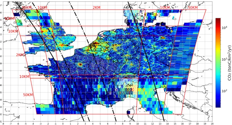
Figure 1. Maps of the IER annual emissions interpolated over the domain of the CHIMERE model. Point sources are indicated by black dots, and administrative regions are shown using thin black lines. The grid of the model is defined by subdomains with several resolutions (r × s km2, where r and s are 2, 10 or 50 km), and their boundaries are represented by the red lines. The thick black lines depict the edges of the satellite tracks corresponding to the synthetic data used in this study (300 km swath: dash-dotted line; 900 km swath: solid line).
2 Inverse modeling system and OSSEs
In the following sections, we describe the different structural elements of the analytical inversion system: the gridded in-ventories used to define the point or area sources to be con-trolled and to map their emissions (Sect. 2.2), the simulation of the atmospheric CO2 and XCO2 signatures of the
con-trolled sources using the CHIMERE atmospheric transport model, and the matrix computation of the posterior uncer-tainties in the emissions (Sect. 2.1.1 and 2.3). We also de-scribe the observations and parameters chosen for the OSSEs in this study: the XCO2 observation sampling and errors
(Sect. 2.1.2) and the prior uncertainties in the emissions, nat-ural fluxes and boundary conditions (Sect. 2.4). New OSSEs with the analytical inversion system can easily be conducted with other options for these observations and parameters. However, for the sake of clarity, the descriptions of the com-ponents of the inversion system and of the options for the OSSEs are intertwined.
2.1 XCO2: transport model simulations and
pseudo-data
2.1.1 Simulations of CO2and XCO2with the
CHIMERE model
To compute the 4D CO2 signatures of surface CO2 fluxes
in the study domain for March and May 2016 as well as of the domain CO2boundary conditions, we use the CHIMERE
regional atmospheric transport model (Menut et al., 2013). This Eulerian mesoscale model was designed to simulate pol-lution (Pison et al., 2007) but has also been used for CO2
atmospheric inversions and, in particular, for city-scale in-versions of the emissions from Paris (Bréon et al., 2015; Staufer et al., 2016; Broquet et al., 2018). It has shown high skill in simulating the daily and synoptic variability in the at-mospheric CO2concentrations at European CO2continuous
measurement sites (Patra et al., 2008).
The domain of our CHIMERE configuration covers most of western Europe (Fig. 1) between the latitudes ∼ 42◦N (northern Spain) and ∼ 56◦N (northern Germany) and be-tween the longitudes 6◦W (eastern Ireland) and ∼ 17◦E (eastern Germany). The horizontal resolution of the zoomed grid of this configuration ranges from 2 to 50 km, with the 2 km × 2 km resolution subdomain being appropriate to simulate the atmospheric signature of a dense network of
sources in northern France, Belgium, the Netherlands, Lux-embourg and western Germany. The zoom and extent of the CHIMERE grid link the simulation of CO2 at local scales
in this area of interest with the transport of CO2 at the
Eu-ropean scale while mitigating the computational cost. The model has 29 sigma vertical layers that extend from the surface to 300 hPa. Model concentration outputs are aver-aged at the hourly scale. The meteorological forcing is from the 9 km × 9 km and 3 h resolution analysis of the European Center for Medium-Range Weather Forecasts (ECMWF). These 3-hourly fields are interpolated at the spatial and tem-poral resolution of CHIMERE. The CO2concentrations used
to impose the conditions at the initial time and at the lat-eral and top boundaries of the CHIMERE domain are from the analysis of the Copernicus Atmosphere Monitoring Sys-tem (CAMS; Inness et al., 2019) at ∼ 16 km resolution. The products used to impose surface CO2fluxes in the model are
detailed below in Sect. 2.2.
XCO2 observations and the corresponding signatures of
fluxes are simulated from the CO23D fields from CHIMERE
at 11:00 LT. For the sake of simplicity in the OSSEs con-ducted here, as we use synthetic data only and a rather sim-ple modeling of the spaceborne observation, the computa-tion of XCO2assumes that the vertical weighting function
of the CO2column-averaging (kernel) is vertically uniform.
For a given model pixel at latitude “lat” and longitude “long”, XCO2is thus computed from the vertical average of the CO2
mole fractions simulated by the model: XCO2(lat, long) =
RPsurf
Ptop CO2(lat, long, P ) dP + CO2(Ptop)Ptop
Psurf(lat, long)
, (1)
where P designates the atmospheric pressure, Psurfis the
at-mospheric surface pressure and Ptop(300 hPa) is the pressure
at the top boundary of the model. For pressures lower than Ptop, we assume that the CO2concentrations equal the
hor-izontal average of the top-level mixing ratios in CHIMERE (CO2(Ptop)). Indeed, we do not expect significant spatial
gra-dients of CO2over the simulation domain in the upper
atmo-sphere. This is supported by the lack of signal in our simu-lations of the atmospheric signatures of the surface fluxes in the upper layer of the model.
2.1.2 XCO2pseudo-data sampling and error
As detailed in Sect. 2.3, the OSSE framework of the inver-sions requires the location and time of the individual XCO2
data, and the associated error statistics, but not the explicit values of the synthetic observations themselves. In this study, we consider pseudo-satellites with a low Earth orbit (LEO) whose altitude and inclination parameters are similar to those of the A-Train (705 km and 98.2◦, respectively; Parkinson et al., 2006). The satellite observations are assumed to occur at 11:00 LT in the morning. Successive tracks of a single
satel-lite on this orbit are separated by ∼ 25◦. However, we do not study the potential of a specific satellite nor that of a con-stellation of such LEO satellites depending on their number. Furthermore, this study focuses on results at the scale of 6 h. Therefore, for any day, it considers single satellite tracks that do not correspond to a specific position of a satellite on the chosen orbit: when studying the emissions of the Paris urban area, we use the track that is nearly centered on this city ev-ery day, and various swaths are considered to study the sen-sitivity of the results to this parameter (Sect. 3.2.2). For the study of results for the ensemble of sources contained within the 2 km subdomain (Sect. 3.3), we use a track centered over Belgium every day and a 900 km swath to ensure a full cov-erage of the plumes from these sources (the sensitivity to a realistic range of swath widths is not investigated in this sec-ond set of analyses).
Our OSSEs assess the impact on the inversion results of the measurement noise from the satellite instrument only, ig-noring the errors associated with the radiative transfer inverse modeling for the retrieval of the XCO2data from the radiance
measurements (Buchwitz et al., 2013a; Broquet et al., 2018), in particular any “systematic error”. Thus, the errors on the XCO2data at the spatial resolution of the measurements are
assumed to be Gaussian, unbiased and uncorrelated in space or time. The distribution of the standard deviation (SD) for these errors is also assumed to be uniform; therefore, these errors are summarized by a single value of SD (denoted as the data precision hereafter).
A large number of scenarios are tested for the ob-servation specifications: the precision on the individual XCO2 data varies between 0.3 and 2 ppm, and the
spa-tial resolution of the ground pixels can take the follow-ing values: 2 km × 2 km (longitude × latitude), 2 km × 3 km, 3 km × 3 km, 3 km × 4 km and 4 km × 4 km. The reference is a precision of 0.6 ppm and a spatial resolution of 2 × 2 km2. These values are similar to the characteristics of the simula-tion of CO2M data used in the study of Wang et al. (2020). When studying the sensitivity of the results over Paris to the swath of the instrument, the swath is varied from 100 to 600 km, with a reference value of 300 km.
2.2 CO2fluxes
2.2.1 Maps and time series of anthropogenic emissions and natural fluxes
High-resolution maps of anthropogenic emissions are needed to define appropriate point and area sources to be controlled by the inversion. High-resolution maps of anthropogenic and biogenic fluxes are also needed to distribute the controlled local to regional budgets of these fluxes on the spatial grid of the CHIMERE model. Finally, such maps are needed to pro-vide insights into the typical budgets of fluxes at the control resolution and, thus, to quantify the prior uncertainty in these budgets with a suitable order of magnitude.
The anthropogenic CO2emissions are extracted from
sev-eral datasets compiled by IER (Pregger et al., 2007; Thiru-chittampalam et al., 2012). These datasets provide maps of the annual budgets per sector of anthropogenic activity over different domains and at different spatial resolutions. We have merged and re-gridded them to derive a map of the annual budgets of emissions over the entire grid of the CHIMERE configuration. The emissions corresponding to France and Germany are extracted from the respective IER national maps for 2005 at a 1 min resolution, whereas emis-sions in Belgium, Luxembourg and the Netherlands are de-rived from an IER 1 km product covering northern Europe for 2005. The IER 5 km resolution map covering the whole of Europe for 2008 is used for the emissions over the rest of the domain. The gridded area sources in the IER maps are in-terpolated on the CHIMERE grid, but the large point sources are relocated as point sources in individual CHIMERE grid cells. We then derive the hourly emission maps from the an-nual emission map by applying the convolution of IER typ-ical temporal profiles specific to each country and sector. These profiles include seasonal, daily and diurnal variations of emissions for large sectors such as traffic, power demand, domestic heating or air-conditioning (Pregger et al., 2007).
The IER maps for France, Germany, northern Europe and the whole of Europe correspond to annual budgets for years (2005 and 2008) that can be different from one area to an-other and that are different from the year chosen for the atmo-spheric transport and for the natural fluxes (2016). This could raise some inconsistencies if assimilating real data into the inversion. However, this study is based on OSSEs with some strong simplifications regarding the observation system, as the overarching target is a general understanding of the be-havior and potential of the inversion. This requires the use of a high-resolution and realistic distribution of the emissions in space and time but not a precise estimate of their amplitudes for a given year.
The land surface natural fluxes are derived from 8 km res-olution simulations made with the Vegetation Photosynthe-sis and Respiration Model (VPRM) for the year 2016. This prognostic model delivers hourly values of net ecosystem ex-change (NEE) by assimilating satellite and meteorological data (Mahadevan et al., 2008). These values of NEE are in-terpolated over the CHIMERE area at the hourly timescale. Natural ocean fluxes are ignored.
2.2.2 Controlled areas
The resulting hourly maps of anthropogenic CO2emissions
for spread sources and large point sources are decomposed spatially to define the areas for which hourly emission bud-gets are controlled by the inversion: large point sources, cities, remaining parts of regions from which point sources and cities have been extracted (covering diffuse emissions only), and full regions where point sources and cities are not controlled separately but are combined with diffuse
emis-sions. Hourly budgets of the natural fluxes are controlled for full regions only, with the regions used for the control of an-thropogenic and biogenic fluxes being identical.
The definition of the regions is done considering the whole domain. It corresponds to administrative regions of France, Belgium, the Netherlands, Luxembourg and Germany, and to three additional large “regions”: the UK, Switzerland and the rest of the domain. This subdivision results in 67 regions (Fig. 1). These 67 regions correspond to the spatial resolution of the natural fluxes in the inversion.
Point sources and cities are controlled individually in the 2 km resolution part of the CHIMERE grid only (Sect. 2.1.1; Fig. 1). In the 39 regions entirely comprised within this sub-domain, we individually control the 84 point sources (e.g., factories, power plants) whose annual emissions are larger than 0.2 MtC yr−1. The maps of the remaining emissions (ex-cluding these point sources) in each of these 39 regions are then processed to extract large urban areas to be controlled independently, ensuring at least one controlled urban area per region, and that no controlled urban area overlaps two dif-ferent regions. An algorithm of pattern recognition has been designed for such an extraction, with the idea that urban ar-eas correspond to clusters of adjacent high-emitting pixels (also followed by Wang et al., 2019). After having applied a Gaussian filter to smooth the spatial distribution of the emis-sions, the large urban areas are defined by a label-connecting algorithm (Stockman et al., 2001) that identifies the clusters of adjacent points whose emissions are above a predefined threshold. As the density and extension of cities vary consid-erably amongst the different regions, the parameters of the pattern recognition algorithm, i.e., the standard deviation of the Gaussian filtering and the emission threshold, are differ-ent for each region to ensure that each region contains at least one controlled urban area (Fig. 2). As a result, we identify 152 controlled urban areas within the 2 km resolution subdo-main. They are characterized by a wide range of budgets and spatial spread of their emissions, their annual budgets range between ∼ 0.07 and ∼ 9.9 MtC yr−1(with a mean and a stan-dard deviation of ∼ 0.8 and ∼ 1.5 MtC yr−1, respectively), and their areas range from ∼ 8 to ∼ 2400 km2 (with a me-dian value of ∼ 240 km2).
The remaining emissions, after having extracted the large point sources and urban areas in the 39 regions, are con-sidered to be diffuse and are hereafter referred to as the “countryside” emissions. The inversion controls their bud-gets in each region. The analysis of the results at the regional scale for these 39 regions will consider either the country-side emissions only (i.e., focusing on the individual control variables) or their aggregation with the emissions from the point sources and cities within the same region (i.e., consid-ering the full geographical extent of the regions). The inver-sion also directly controls the total budget of the emisinver-sions for the 28 regions that are not fully comprised in the 2 km subdomain (most of these 28 regions do not overlap this sub-domain at all). Overall, the control of countryside or total
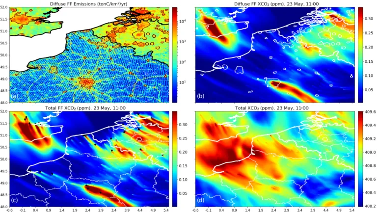
Figure 2. IER emission maps interpolated over northern France, western Belgium and the London area (a). We have represented the anthro-pogenic emission sources without point sources (“area emissions”). Red curves depict the boundaries of the city clusters defined by a pattern recognition algorithm (Sect. 2.2.3). Panel (b) shows the simulations of XCO2(ppm) that are produced by the area emissions. Panel (c) shows
the simulations of XCO2(ppm) that are produced by the total anthropogenic emissions. Panel (d) shows simulations of XCO2(ppm) on 23
May at 11:00 LT that are produced by the combined anthropogenic, natural and boundary fluxes between 05:00 and 11:00 LT. For the sake of clarity, these figures do not show the whole 2 km resolution subdomain of CHIMERE; instead, they illustrate the patterns seen over this subdomain.
regional emissions adds 67 controlled areas (corresponding to the 67 regions) for the anthropogenic emissions so that the inversion controls the hourly budgets of anthropogenic emis-sions for 303 areas (84 point sources, 152 urban areas and 67 countryside or regional areas) and the hourly budgets of natural fluxes for 67 areas.
2.3 Analytical flux inversion 2.3.1 Theoretical framework
The inversion system follows a traditional analytical inver-sion approach based on the Bayesian formalism and assum-ing that error statistics follow Gaussian distributions (Taran-tola et al., 1987; Broquet et al., 2018). The system controls factors that scale the hourly budgets of the different control areas for the anthropogenic and biogenic fluxes defined in Sect. 2.2.2. It also controls a single scaling factor applied to the CO2field used to impose the initial, lateral and top CO2
boundary conditions of the model, as such boundary condi-tions generally bear important large-scale uncertainties that can impact the estimates of sources within the domain (Bro-quet et al., 2018). In the OSSEs of this study, the inversion
periods for each day in March or May 2016 cover the 6 h (05:00–11:00 LT) before 11:00 LT, when the satellite obser-vations are supposed to be made. The number of control vari-ables (2221 = 370 controlled areas × 6 time slots + 1 control variable for the boundary conditions) is sufficiently small to solve the inverse problem analytically. However, building the matrix H that encompasses the atmospheric transport opera-tor and that is described below (Sect. 2.3.2) requires a large computational burden.
For a given inversion period, we define the control vector x as the set of controlled scaling factors for the hourly flux budgets and the boundary conditions. The prior uncertainty in x is assumed to follow a Gaussian distribution and to be unbiased. Thus, it is characterized by the uncertainty covari-ance matrix B.
In this study, the observation vector y is defined by the XCO2concentrations in the transport model horizontal grid
cells sampled by the observations. The simulation of y based on a given estimate of x is given by the linear observa-tion operator H: x → y = Hx, which chains three operators. The first operator Hdistrdistributes the controlled hourly
provides the spatial and temporal mapping of the boundary conditions whose scaling factor is controlled by the inver-sion. The second operator Htranspis the atmospheric transport
from the emissions and the boundary conditions to the full CO2and XCO2fields. Finally, the third operator Hsample
per-forms the XCO2sampling at the location of the XCO2data
(Sect. 2.1.2). Differences between Hx and observed values for y arise due to (1) uncertainties in x and (2) the combina-tion of errors in the observacombina-tion operator and in the observa-tion data that are together referred to as “observaobserva-tion errors”. The errors from the observation operator are strongly asso-ciated with the atmospheric transport model errors (Houwel-ing et al., 2010; Chevallier et al., 2010) as well as with the discretization and spatial resolution of the transport and in-version problems, which raise representation and aggrega-tion errors (Kaminski et al., 2001; Bocquet et al., 2011). As-suming that they follow Gaussian and unbiased distributions like the prior uncertainties, these observation errors are fully characterized by the observation error covariance matrix R. The H, B and R matrices must be explicitly estimated in the analytical inversion framework (Sect. 2.3.2 and 2.4).
The Bayesian theory (Tarantola et al., 1987) states that the statistics of the knowledge on x knowing (i) the prior esti-mate of x, (ii) the observed values for y and (iii) H as a link between the x and y spaces, follow a Gaussian and unbi-ased distribution. Thus, the uncertainty in such a posterior estimate is fully characterized by the posterior uncertainty covariance matrix A given by
A =hB−1+HTR−1Hi−1 (2) The analysis of A and its comparison to B, aggregated or not over different spatial and temporal scales, are the criti-cal diagnostics in this study to assess the potential of inver-sions assimilating XCO2 images. The score of uncertainty
reduction for a given flux budget is a common indicator for evaluating the performance of an observation system. It is defined as the relative difference between the SD of the prior (σprior) and posterior (σpost) uncertainties in this flux budget
(UR = 1 − σpost
σprior). If the assimilation of satellite observations
perfectly constrains a given flux budget, the corresponding UR equals 100 %. If this assimilation does not provide any information on the flux budget, UR equals 0 %.
2.3.2 Building the observation operator matrix H The analytical inversion system is essentially built on the explicit computation of H = HdistrHtranspHsample. The
differ-ent columns of H correspond to the signatures (or “response functions”) in the observation space of the different control variables, i.e., of the different hourly emissions for each con-trol area, and of the boundary conditions. They are computed by applying the sequence of operators Hdistr, Htranspand then
Hsample to each control variable set to 1, keeping the
oth-ers null (Broquet et al., 2018). Hdistr is defined based on
the flux maps detailed in Sect. 2. Htranspcorresponds to the
CHIMERE model and to the vertical integration of CO2into
XCO2 presented in Sect. 2.1.1, while Hsample corresponds
to the sampling, on the transport model grid, of the simu-lated XCO2 values according to the spatial distribution of
the pseudo-observations (Sect. 2.1.2). A generalized H is ac-tually stored for the analytical inversion system to anticipate any option for Hsample, by recording the full CO2and XCO2
fields from the application of HdistrHtransp to each control
variable, i.e., the full CO2and XCO2signatures of each
con-trol variable.
2.4 Practical implementation of the OSSEs
While, in principle, R should characterize both the errors in XCO2data and the errors from the observation operator H,
this study focuses on the impact of the observation sampling and errors only. It ignores the errors from the observation op-erator. Moreover, the observation errors are restricted to the measurement noise, which is uncorrelated in space and time as detailed in Sect. 2.1.2. Thus, the different R matrices used for the OSSEs (depending on the observation sampling and noise) are all diagonal. The errors on the individual pseudo-observations are described by a uniform precision (σXCO2)
depending on the chosen satellite configuration (Sect. 2.1.2). However, the observation vector y is defined by the transport model grid rather than by the precise location and coverage of the data. Therefore, the diagonal elements of R follow the aggregation of nobs pseudo-observations with uncorrelated
errors (where nobsis potentially greater than 1) within each
model grid cell corresponding to an element of y, so that the resulting SD of the errors for this element is given byσ√XCO2
nobs.
Prior estimates of anthropogenic emissions and biogenic fluxes are generally provided by inventories and ecosystem model simulations such as those used here in Hdistr to
dis-tribute the fluxes at high resolution. B should characterize un-certainties in such products and is thus set with values corre-sponding to typical relative uncertainties in the budgets from the maps detailed in Sect. 2.2.1. Prior estimates of the bound-ary conditions for regional inversions are usually interpolated from large-scale analysis or inversions. Such products can bear significant large-scale errors at the boundaries of Europe (Monteil et al., 2020). We reflect this by setting the standard deviation of the prior uncertainty in the scaling factor for the boundary conditions in B (see below). When constructing the B matrices in all of our OSSEs, we assume that there is no correlation between the prior uncertainties associated with different controlled emission areas or between these un-certainties and that associated with the boundary conditions. The spatial correlations of the uncertainties in anthropogenic emission inventories is a complex topic, and the current lack of characterization for such correlations led to such a conser-vative setup (Wang et al., 2018; Super et al., 2020). However, we model the temporal correlations between prior uncertain-ties in scaling factors associated with different hourly natural
or anthropogenic flux budgets of the same controlled emis-sion area by using an exponentially decaying function with a correlation timescale τ (like, for instance, Bréon et al., 2015): ρi,j=e−
|j −i|
τ , (3)
where j and i are the indices of 2 corresponding hours. The SD of the prior uncertainties in the scaling factors for the dif-ferent hourly budgets of the same controlled area are fixed to an identical value σhour. Finally, we assume that the SD of
the prior uncertainties in scaling factors for the 6 h budgets of the natural fluxes or of the anthropogenic emissions from a controlled area from 05:00 to 11:00 LT (to be applied to the budgets from the IER and VPRM products presented in Sect. 2.2.1 and used to build Hdistr) is fixed to a value σBudget
that is the same for all control areas: typically 50 % or 100 % of the 6 h budgets. The SD of the prior uncertainties in the scaling factors for the hourly budgets of the controlled ar-eas σhour are then derived based on these different
assump-tions. The reference parameters for B are fixed to τ = 3 h and σBudget=50 %. Despite the differences between the
tempo-ral variations of the hourly emissions from one control area to another or between natural and anthropogenic fluxes in Hdistr, these SD values show a negligible variation of less
than 1 %, and when considering the reference setup for B, σhour∼65 %. The sensitivity of the inversion to the values of
σBudget and τ is assessed in Sect. 3.2.3. Finally, we use 1 %
for the SD of the prior uncertainty in the scaling factor asso-ciated with the boundary conditions (i.e., typically an uncer-tainty of ∼ 4 ppm in the average boundary conditions). This value is quite pessimistic, but some tests in which this value was varied (not shown) demonstrate a very weak sensitivity of the results for the fluxes to this parameter.
3 Results
3.1 High-resolution simulations of XCO2
Previous sections documented how, for each 6 h period, the inversion system exploits the simulated XCO2 fields
at 11:00 LT to constrain each hourly budget of the anthro-pogenic or natural fluxes of the controlled areas between 05:00 and 11:00 LT. The CHIMERE full XCO2simulations
between 05:00 and 11:00 LT with the anthropogenic emis-sions, natural fluxes and/or domain boundary conditions de-tailed in Sect. 2.1 and 2.2 are used in this section to compare the overall signatures of these components and of the con-trolled areas as well as to discuss their overlapping. Figure 2b shows the XCO2 signatures of all the anthropogenic
emis-sions in the domain except those from the 84 point sources controlled individually by the inversion in the 2 km resolu-tion subdomain (that are illustrated in Fig. 2a). Figure 2c integrates the XCO2 produced by the 84 point sources and
shows the signature of all the anthropogenic emissions. Fi-nally, Fig. 2d displays the superposition of the XCO2
sig-natures of all the anthropogenic emissions, of the natural fluxes and of the boundary conditions. For all of these fig-ures, XCO2values are taken at 11:00 LT and are provided by
simulations between 05:00 and 11:00 LT on 23 May which is a day of strong northwest wind (∼ 10 m s−1over Paris at 700 m above ground level).
The strong plumes from the megacities of Paris and Lon-don are easily distinguished when considering the signature of anthropogenic emissions in Fig. 2b and c, with their ampli-tude exceeding 0.3 ppm at 100 km downwind of these cities and with sharp gradients of XCO2at their edges. The
rela-tive narrowness, extended length and small intensity of the plumes shown in Fig. 2b and c are explained by the mag-nitude of the wind speed on 23 May. The characteristics of those plumes vary considerably with respect to the wind speed, and the inversion results are strongly impacted by this parameter (Sect. 3.2.1; Broquet et al., 2018).
Figure 2b and c also show that the overlapping of plumes from urban areas in Belgium and in the Netherlands produces XCO2 patterns whose amplitudes are comparable to those
of the plumes from Paris and London. However, due to the urban density of those countries, the level of distinction be-tween the individual signatures of the different cities is weak. If we exclude Paris, northwestern France has a much less dense urban fabric with scattered cities of small extents. This sparse distribution allows the relatively weak plumes from cities to be visible, whereas the more diffuse XCO2
signa-tures of the countryside emissions do not form any distin-guishable patterns (Fig. 2b).
The comparison between Fig. 2b and c highlights the plumes from some of the large 84 point sources within the 2 km resolution subdomain (Sect. 2.2.2). The amplitude of these plumes can locally reach that of Paris but such an in-crease above the background occurs on a much smaller ex-tent: for instance, that of the power plant close to Dunkerque (∼ 51◦N, ∼ 2.3◦E) on the northern French coast reaches 0.4 ppm, but its width does not extend to more than 5 km (Fig. 2c). The capacity of our high-resolution transport model to simulate narrow XCO2plumes from point sources or
ur-ban areas distinct from that of neighboring or surrounding sources is revealed by the example of several point sources in Belgium as well as that of the oil refinery of Grand-puits (48.59◦N, 2.94◦E) whose plume stands out of the large plume from the Paris urban area (Fig. 2c). The 2 km resolu-tion zoom of the model grid allows one to distinguish those features that would be blurred in a coarser-resolution trans-port model.
When including the XCO2produced by the natural fluxes
and the boundary conditions, identifying the features pro-duced by the anthropogenic emissions is more difficult (Fig. 2d). The atmospheric signatures of Paris, London and the high-emitting power plants are hardly differentiated from patterns produced by the boundary conditions and natural fluxes, even though they are still visible. The isolated plumes of low amplitudes from scattered cities with small extents
and low emission budgets can hardly be seen. The boundary conditions and the natural fluxes tend indeed to produce sig-natures whose amplitude is often larger than, or at least com-parable to, that of the signal from the anthropogenic emis-sions, with which they interfere. This blurs this signal of the anthropogenic emissions, especially when the emissions are diffuse. Boundary conditions and natural fluxes are, how-ever, much more distributed homogeneously than the anthro-pogenic emissions, which are localized over a small fraction of the surface. As a consequence, the boundary conditions and the natural fluxes produce smooth XCO2fields (Fig. 2d),
whereas the anthropogenic emissions produce heterogeneous fields with finer structures and sharper gradients (Fig. 2c). Therefore, the separation between the two types of fluxes could rely on the differences in terms of spatial scales of their atmospheric signatures or on a precise knowledge of the at-mospheric transport patterns.
This first qualitative overview of the atmospheric signa-tures could imply that the ability to quantify the budgets of emissions for the two megacities, for most of the 84 large point sources, and for large regions in the northeast should be much larger than for the individual urban areas in most of the domain or for the countryside emissions. However, this diagnostic relies on a qualitative assessment of Fig. 2. In Sect. 3.3, we will quantitatively analyze the inversion re-sults as a function of the type of sources.
3.2 Potential of the satellite images for monitoring the anthropogenic emissions of a megacity: sensitivity studies
This section assesses the performance of our inversion as-similating XCO2images to monitor the anthropogenic
emis-sions from the Paris area as a function of the wind conditions; as a function of the XCO2observation precision, resolution
and swath; and as a function of the configuration of the prior error covariance matrix B. The results are relative to the in-version control area that covers most of the Paris urban area (Fig. 2a). The analysis is based on sixty-two 6 h inversion tests with satellite images nearly centered on this area for each day of March and May 2016. With the reference 300 km wide swath, such images cover the plumes from the Paris ur-ban area entirely under most wind conditions (Broquet et al., 2018). In the following, the wind speed is characterized by its averaged value at 700 m above ground level over the inver-sion control area corresponding to Paris and over the period corresponding to the chosen diagnostic: over 05:00–11:00 LT when analyzing the uncertainty in the budgets of the emis-sions corresponding to the full 6 h period of inversion or over the [hh,11:00] time interval when analyzing the uncertainty in the hourly budget of the emissions between the hours hh and hh+1.
3.2.1 Impact of the wind speed
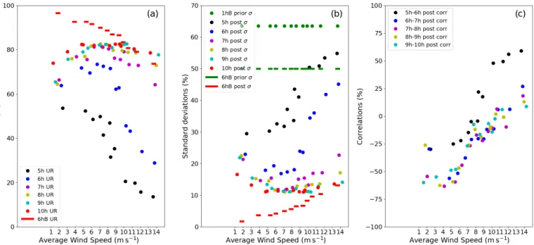
A first set of inversions is conducted with the reference val-ues for the precision, resolution and swath of the satellite observation and for the parameters of the prior uncertainty (0.6 ppm, 2 × 2 km2, 300 km, 50 % and 3 h, respectively). These inversions are applied to 12 different days in March 2016 which present a range of average wind speeds from 2 to 14 m s−1 (Fig. 3). We investigate results in winter, when the amplitudes of the biogenic fluxes are low, to mitigate the influence of these fluxes (and of their variability) on the URs for the Paris emissions. Note that the time profiles modeling the variability in the anthropogenic emissions ignore day-to-day variations (except between weekend and working day-to-days) which almost removes the influence of the variability in these emissions when studying results in March only. Results are presented in terms of prior and posterior uncertainties in both the 1 and 6 h budgets of emissions from the Paris urban area. The directions of the wind are predominantly meridional so that the selection of the swath has no impact. The main anal-ysis and conclusions in this section are similar to that of Bro-quet et al. (2018), so we present them briefly.
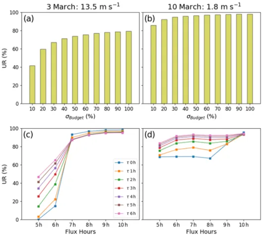
Results in Fig. 3 illustrate the fact that higher wind speeds lead to smaller uncertainty reductions for the 6 h emission budgets: on 3 March, the average wind speed is 13.5 m s−1 and the UR with the reference values for the precision, res-olution and swath is 74 %; whereas on 10 March, the aver-age wind speed is ∼ 1.8 m s−1and the UR is 97 % (Fig. 3a). Stronger winds decrease the UR because, due to an increased atmospheric dilution, the amplitude of the city plume is smaller which decreases the signal-to-noise ratio for the in-version. However, when considering the UR for hourly emis-sions, this rule may not apply for wind speeds lower than 6 m s−1. For this range of wind speeds, the posterior un-certainty in 09:00–10:00 LT and 10:00–11:00 LT emissions increases with decreasing wind speed (Fig. 3b). The inver-sion system shows difficulties in distinguishing the atmo-spheric signatures produced by consecutive hourly emissions because these signatures have a significant overlap when the wind speed is low. This explanation is confirmed by the nega-tive correlations found between the uncertainties in consecu-tive hourly emissions, as the magnitude of these negaconsecu-tive cor-relations increases when the wind speed decreases (Fig. 3c). Important negative correlations also explain that 6 h emis-sion budgets are better constrained for low wind conditions, even though hourly emissions can be poorly constrained. The overestimation of some hourly emissions is compensated for by the underestimation of other hourly emissions.
The uncertainty reductions for 1 h and 6 h budgets are high for a large range of wind values: in all the tests here, the URs for the 6 h budgets are above 74 % and the UR for the 1 h budgets after 07:00 LT are above 62 % (Fig. 3a). Concerning the 1 h budgets of the 05:00 to 07:00 LT emissions, the corre-sponding URs significantly decrease for wind speeds above 10 m s−1. In particular, the UR for the 5:00 to 6:00 LT
emis-Figure 3. Uncertainty reductions (UR) from a 50 % prior uncertainty on the 6 h budgets of the Paris emissions for 12 d characterized by different average wind speeds over Paris (a). The UR for hourly and 6 h budgets of the Paris emissions are shown using colored dots and red segments, respectively. In panel (b), the prior vs. posterior uncertainties on 1 h emissions (colored dots) and 6 h emissions (green and red segments) of Paris are shown. In panels (a) and (b), the colors of the dots represent the hour of the corresponding 1 h budget; the green dots represent the prior uncertainties on the 1 h emissions (1 hB prior σ ) which are derived from 50 % prior errors on the 6 h budgets (6 hB prior σ )and by considering temporal prior correlations of 3 h. Panel (c) shows correlations between posterior uncertainties in two consecutive 1 h emissions (colored dots). Results are computed with a retrieval resolution of 2 km × 2 km, a precision of 0.6 ppm and a swath of 300 km.
sion drops below 20 % above this value for the wind speed. This behavior is consistent with the fact that the signatures of emissions occurring well before the satellite overpass have been much more diffused through atmospheric transport at the observation time than that of later emissions.
3.2.2 Impact of the precision, resolution and swath of the satellite images
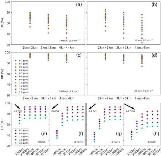
Figures 4a–d show the URs for the 6 h emission budgets of 3 March (with strong wind), 10 March (with low wind), 23 May (with strong wind) and 27 May (with low wind). This figure corresponds to a second set of inversions per-formed with the range of options for satellite data preci-sions and resolutions presented in Sect. 2.1.2 but with the observation swath, the relative prior uncertainty in the 6 h budgets of fluxes and the correlation length scale for the prior uncertainties in hourly fluxes fixed to the reference values (300 km, 50 % and 3 h, respectively). The sensitivity of the UR to the measurement precision and resolution in-creases with stronger winds. For example, on 27 May (un-der weak wind) and 23 May (un(un-der strong wind), the UR in-creases by 16 % and 48 %, respectively, between inversions with 2 ppm precision data and inversions with 0.3 ppm pre-cision data (at the resolution of 2 km × 2 km). For those 2 d, the UR decreases by 6 % and 20 % between inversions with 2 km × 2 km resolution data and inversions with 4 km × 4 km
resolution data (with a precision of 0.6 ppm), respectively. The comparison between results on 3 and 10 March confirms such a high sensitivity under stronger winds. It is related to the fact that the slope of the convergence of the UR towards 100 % with better precision and finer resolution is smaller with low wind speeds, which generate higher UR than high wind speeds. For similar reasons, the sensitivity to the pre-cision decreases at finer resolution, and the sensitivity to the resolution decreases with better precision (Fig. 4a–d).
The comparison between results obtained when doubling the random measurement error of the individual observa-tions and when multiplying the value of their spatial res-olution by 4 provides insights into the exploitation of the fine-scale patterns of the XCO2 image by the inversion.
In-deed, both changes result in doubling the resulting error at coarse resolution, but doubling the random measurement er-ror at fine resolution conserves the capability to exploit in-formation at this fine resolution, unlike coarsening the spa-tial resolution of the image. Figure 4a–d show that scores of UR with 2 km × 2 km resolution and 2 ppm precision data are extremely close to those with 4 km × 4 km resolution and 1 ppm precision data. URs with 2 km × 2 km resolution and 1.2, 1, 0.8 or 0.6 ppm precision data are also similar to URs with 4 km × 4 km resolution and 0.6, 0.5, 0.4 or 0.3 ppm pre-cision data, respectively. This indicates that the inversions here do not really take advantage of the information on the fine-scale patterns of the plume from Paris.
Figure 4. Uncertainty reductions (UR) from a 50 % prior uncertainty for the 6 h budgets of the Paris emissions. In panels (a)–(d), results are displayed for 4 different days characterized by different wind speeds, for different spatial resolutions of the satellite data (x axis) and for different precisions (colored markers). In panels (a)–(d), results are generated by considering a swath of 300 km. In panels (e)–(h), results are displayed for 4 different days characterized by different wind speeds, for different swaths of the satellite data (x axis), for different precisions (colored markers) and for a resolution of 2 km by 2 km.
A third set of inversions is conducted to study the sensi-tivity of the results to the width of the satellite swath while keeping all other observation and inversion parameters at ref-erence values. This sensitivity is modulated by the wind con-ditions: the speed and direction of the wind control the spread and position of the plume and, thus, the value of the swath which fully covers the extent over which the amplitude of the plume is significant for the inversion, i.e., the value of the swath above which the results no longer change (Fig. 4e– h). This threshold value of the swath is lower for lower wind speed. For wind directions across the satellite track, the URs for the 6 h emissions of the Paris area are no longer sensitive to the increase in the swath above a value of 100 and 400 km for wind speeds lower than 8 and 9 m s−1, respectively. The sensitivity to the swath is null (except if considering very low values for the swath of the order of the width of the plume from Paris) for wind directions along the satellite track as we consider satellite tracks centered on Paris.
3.2.3 Impact of the definition of the prior uncertainties in the CO2fluxes
The prior uncertainty covariance matrix B has a strong influ-ence on the scores of posterior uncertainties when its “ampli-tude” is comparable to or much larger than that of the HTRH matrix (see Eq. 2), i.e., once the prior uncertainties are com-parable to or much larger than the projection of the observa-tion errors in the control space. The relative prior uncertainty in the 6 h emission budgets (σBudget, Sect. 2.4), which
char-acterizes the diagonal of B, is one of the critical drivers of the relative weight given by the inversion to the prior information and to the observations.
Thus, in a fourth set of inversions, we analyze the sen-sitivity of the inversion results for 6 h emission budgets to σBudget, with values for this parameter ranging between 0 %
and 100 %. This set of inversions uses the reference values of the observation parameters and for the temporal autorelation of the prior uncertainties. Figure 5a–b show the cor-responding results on 3 March (under strong wind) and on
10 March (under low wind) to highlight the dependence of this sensitivity to the wind speed. The curves of UR as a function of σBudgethave an inflection point for values around
50 %. For low values of σBudget, the UR is sensitive to this
pa-rameter, the posterior uncertainty balancing the prior uncer-tainty and the projection of the observation error. For large values, the UR converges asymptotically towards 100 % and the posterior uncertainties are dominated by the projection of the observation error (i.e., the posterior estimate of the emission essentially relies on the top-down information from the observations). The observational constraint on the inver-sion is larger on 10 March than on 3 March as the wind is much lower on the former. As a consequence, the qualitative threshold for σBudgetabove which the URs are not very
sensi-tive to this quantity is smaller on 10 March than on 3 March: 30 % and 50 %, respectively.
These results over Paris suggest an empirical choice of a reference value for σBudget>50 %, in the absence of any
fac-tual knowledge about σBudget. With 50 % as a reference value,
we focus our analysis of the posterior uncertainties on the projection of the information from the observations, and we almost neglect the prior information while retaining an as-sumption regarding the prior uncertainties that could seem consistent or even optimistic compared with series of assess-ment of the errors in inventories for cities at the daily scale (Wang et al., 2020). However, for other cities, for point or area sources with smaller amplitudes, the observational con-straint is lower. The relative weight between the projection of the observations and the prior information is then more balanced than for Paris, and the prior uncertainty still has a significant impact on the posterior uncertainties when using σBudget=50 %. In order to study the pure projection of the
observation errors, results using σBudget=100 % will be
an-alyzed along with those using σBudget=50 % in Sect. 3.3.
The other important parameter defining the B matrix in this study is τ (Sect. 2.4). By construction, the increase in the corresponding autocorrelations in the prior uncertainties at the hourly scale in B does not modify the prior uncertaties in the 6 h emission budgets. However, it can help the in-version crossing the information on different hourly budgets to better constrain the overall budget of emissions. A fifth set of inversions with the reference values for the observation parameters and for σBudget is conducted to test the
sensitiv-ity to τ , with values for this parameter from 0 to 6 h (0 h indicating that there is no temporal correlation in B, and 3 h being the reference value), on 10 and 3 March. The analy-sis shows that the increase in τ hardly impacts the results for the 6 h budgets (not shown) but significantly changes the results for the hourly budgets (Fig. 5c–d). The autocorrela-tion brings informaautocorrela-tion about the temporal distribuautocorrela-tion of the emissions, constraining how the 6 h emission budgets are dis-tributed at the hourly scale. This impact is more significant when the XCO2signatures of the hourly emissions overlap,
i.e., for hourly emissions between 05:00 and 07:00 LT when the wind speed is high and for almost all the hourly emissions
when the wind speed is low. However, this better knowledge about the temporal variations from autocorrelations does not appear to improve the knowledge on the 6 h budgets. 3.3 Potential of satellite images for monitoring
anthropogenic emissions at the regional, city and local scales
This section synthesizes the inversion results at the local (for power plants, industrial facilities) to regional scales over most of the model 2 km resolution subdomain, using a sixth set of inversions assimilating images that cover this sub-domain entirely with a 900 km swath centered on Belgium (Fig. 1). This set of inversions covers all the days of March and May 2016 in order to analyze the impact of the wind speed and of the natural fluxes on the results. The prior relative uncertainties in the 6 h budgets of the emissions are alternatively set to σBudget=50 % and 100 %. These
in-versions use the reference parameters for the observation precision and resolution and for the temporal autocorrela-tion of the prior uncertainties in hourly emissions (0.6 ppm, 2 km × 2 km and 3 h, respectively). Results over most of the 2 km resolution subdomain using different observation spa-tial resolutions and precisions will briefly be discussed in Sect. 4.
3.3.1 Overview of the inversion performance
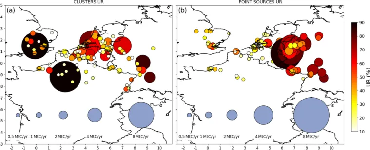
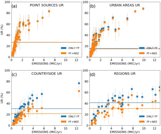
Figure 6 gives a geographical overview of the scores of UR in the 2 km resolution subdomain. The largest scores of UR for 6 h budgets are obtained for the megacities of Paris and London with mean values over the 2 months considered of >80 %. Mean UR can also be >60 % for several cities in Belgium and the Netherlands and for a large number of point sources (power plants and large industrial facilities) within the dense industrial area of western Germany, although these sources are close to each other or to other significant point and area sources.
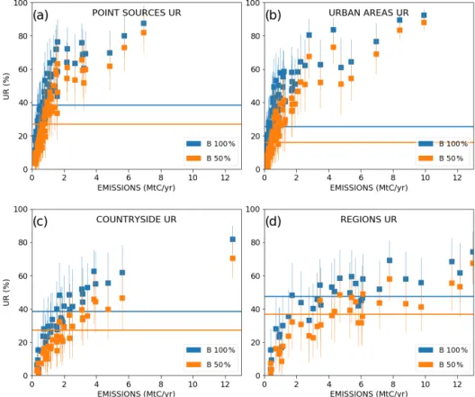
In a general way, the scores of UR increase with the mag-nitude of the emissions (Fig. 7). This increase is more im-portant when considering lower emission values due to the asymptotic convergence of the UR towards 100 % for high emission values (with a point of inflection for sources of ∼2 MtC yr−1 in the curves of Fig. 7). The increase in the UR as a function of the budgets of emissions is different if considering point or area sources. As expected, the largest URs are obtained for narrower sources like point sources (Fig. 7a) and cities (Fig. 7b) which generate plumes with smaller extents but larger amplitudes than diffuse country-side emissions. When using σBudget=100 %, the mean URs
are larger than 50 % for all point sources and cities with an emission rate larger than 2 MtC yr−1, while to achieve 50 % UR, an emission rate of at least 4 MtC yr−1 is needed for regional countryside emissions (Fig. 7c). The gap is even larger when using σBudget=50 %, with mean URs that are
Figure 5. Uncertainty reductions (UR) as a function of the prior uncertainty (x axis) for 6 h budgets of the Paris emissions (a, b). Correlations between the prior errors on hourly emissions have a temporal length of 3 h (see Sect. 2.4). Panels (c) and (d) show the UR for the hourly emissions between 5 and 11 h (x axis) for several temporal lengths defining the correlations between prior errors on hourly emissions (colored dots), with “τ 0 h” referring to an absence of such correlations. Prior uncertainties on 6 h budgets of Paris emissions are taken to be equal to 50 % in panels (c) and (d). Columns represent 2 different inversion days: 3 March 2016 (strong wind) and 10 March 2016 (low wind). All inversion results are computed with a retrieval resolution of 2 km × 2 km, a precision of 0.6 ppm and a swath of 300 km.
systematically larger than 50 % for annual emission budgets of point sources and cities larger than 2 MtC yr−1, but for annual emission budgets of regional countryside emissions larger than 7 MtC yr−1.
When aggregating the results for point sources, cities and countryside emissions at the regional scale, the relative prior uncertainty becomes significantly smaller than the values used for individual sources, as we assume that there is no correlation between their uncertainties: the mean prior un-certainty for the regions is then ∼ 33 % when assuming a 50 % prior error on the 6 h budgets of point sources, cities and countryside areas which make these regions. Moreover, the emission threshold above which the URs for the regional budgets are larger than 50 % becomes 10 and 7 MtC yr−1 when using σBudget=50 % and 100 %, respectively (Fig. 7d).
These thresholds are larger than those corresponding to in-dividual point sources and cities as given above, but the overall performance of the inversion system at the regional scale is better with respect to that of the point sources and cities when analyzing the relative posterior uncertainties: for σBudget=50 %, the mean value is 22 % for the total regional
budgets, whereas it is ∼ 40 % for the point sources’ and cities’ budgets (Fig. A1).
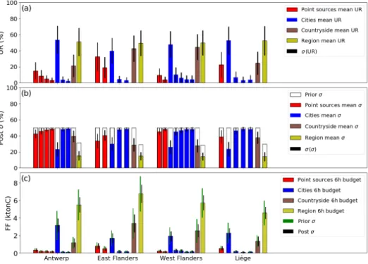
The results for the different types of sources are shown for four regions of Belgium in Fig. 8. This figure provides an illustration of the general results seen in Fig. 7. It shows that the URs for emissions of the largest urban areas (emit-ting more than 2 MtC yr−1) are as high as those for the over-all emissions of their respective region, although the budgets of emissions from these urban areas are much smaller than those of their regions. As suggested above, smaller prior un-certainties in the regional budgets lead to similar URs for cities’ and regions’ budgets, even though the relative pos-terior uncertainties in regional budgets are much smaller (Fig. 8b). When comparing point sources and cities that are characterized by the same prior uncertainty, the relative mag-nitudes of the URs are determined by the relative magni-tudes of the emissions; thus, URs are much higher for the largest urban areas than for point sources and cities that emit much less CO2. However, the comparison between the URs
and emissions of the main cities and countryside areas of the regions of East and West Flanders illustrates that, even
Figure 6. Mean uncertainty reductions (UR) for some city clusters (a) and some point sources (b) across the 62 inversion results for the days of March and May 2016. The areas and colors of the disks represent the annual emissions (MtC yr−1) and the UR (%), respectively. The inversions are performed with a retrieval resolution of 2 km × 2 km, a precision of 0.6 ppm and a swath of 900 km. Prior uncertainties on 6 h budgets of clusters and point sources emissions are taken to be equal to 50 %, and prior error correlations have a temporal length of 3 h.
though they have lower emission budgets in these regions, cities are better constrained than countryside areas. This is in agreement with the enhanced capacity of the inversion sys-tem to monitor city emissions with respect to more diffuse emissions. This figure also qualitatively illustrates the abil-ity of the inversion system to separate neighboring emission sources: the point source and city of Liège (left blue bar for the region of Liège in the figure) contained within the region of Liège are characterized by significant URs even though the point source is within the city of Liège and its plume is completely overlapped by the plume from the rest of the city. We will more systematically and quantitatively analyze the capacity of the inversion to disentangle the signals produced by neighboring sources in Sect. 3.3.3.
The URs for the 6 h emission budgets show an impor-tant variability over the 62 inversion days as illustrated in Fig. 7. When using σBudget=50 %, the standard deviations
of the day-to-day variations of the URs for the point sources, cities and countryside areas, are on average, equal to ∼ 12 %, ∼8.3 % and 12.2 %, respectively. These values are impor-tant with respect to the temporal mean of the values of UR (26 %, 16 % and 27 % when averaging across all the point sources, cities and countryside areas, respectively). These variations are associated with variations in the wind speed at the daily scale, as evidenced for the Paris case in Sect. 3.2.1. However, when considering results for the months of March and May together, they are also driven by the time profiles of the anthropogenic emissions that are characterized by a strong decrease in emissions between March and May due to the reduction of residential heating. Moreover, the UR variability is also determined by that of the uncertainties in
the natural fluxes which are also very different from March to May. The natural fluxes have large negative amplitudes in May when they are dominated by the primary produc-tion and smaller positive amplitudes in March when they are mostly restricted to the heterotrophic respiration. Using con-stant prior relative uncertainties in the natural fluxes (as for the anthropogenic emissions) yields large absolute uncertain-ties in May and low absolute uncertainuncertain-ties in March. Fur-thermore, as the primary production related to photosynthetic processes is mostly driven by the radiative forcing and then by the daily variation in the cloud cover, natural fluxes and their prior uncertainties are also characterized by a strong day-to-day variability during the month of May; this is not the case in March due to a weak day-to-day variability in heterotrophic respiration. Cross sensitivity studies compar-ing the influence of the above drivers (not shown) indicate the predominant influence of the daily variability in the wind speed on the variability in UR for the anthropogenic emis-sions estimates for most sources. This conclusion should, however, be nuanced for some regions and countryside ar-eas where the scores of UR for the anthropogenic emission estimates is highly impacted by the inversion of the natural fluxes and, thus, by the variability in these fluxes, during the month of May (see Sect. 3.3.2. below).
3.3.2 Impact of the uncertainties in the biogenic fluxes The analysis of XCO2 patterns produced by the different
CO2 fluxes (Sect. 3.1) suggests that the large signatures of
the biogenic fluxes in May could impact the monitoring of the anthropogenic emissions. In order to weigh the impact of the uncertainties in biogenic fluxes, we conduct experiments