HAL Id: hal-01236999
https://hal.archives-ouvertes.fr/hal-01236999
Submitted on 8 Dec 2015
HAL is a multi-disciplinary open access
archive for the deposit and dissemination of
sci-entific research documents, whether they are
pub-lished or not. The documents may come from
L’archive ouverte pluridisciplinaire HAL, est
destinée au dépôt et à la diffusion de documents
scientifiques de niveau recherche, publiés ou non,
émanant des établissements d’enseignement et de
From stereoscopic images to semi-regular meshes
Jean-Luc Peyrot, Frédéric Payan, Marc Antonini
To cite this version:
Jean-Luc Peyrot,
Frédéric Payan,
Marc Antonini.
From stereoscopic images to
semi-regular meshes.
Signal Processing:
Image Communication, Elsevier, 2016, 40, pp.97-110.
�10.1016/j.image.2015.11.004�. �hal-01236999�
From stereoscopic images to semi-regular meshes
Jean-Luc Peyrot, Fr´ed´eric Payan and Marc Antonini
Laboratory I3S - University Nice - Sophia Antipolis and CNRS (France) - UMR 7271
Abstract
The pipeline to get the semi-regular mesh of a specific physical object is long and fastidious : physical acquisition (creating a dense point cloud), cleaning/meshing (creating an irregular triangle mesh), and semi-regular remeshing. Moreover, these three stages are generally independent, and processed successively by dif-ferent tools. To overcome this issue, we propose in this paper a new framework to design semi-regular meshes directly from stereoscopic images. Our semi-regular reconstruction technique first creates a base mesh by using a feature-preserving sampling on the stereoscopic images. Afterwards, this base mesh is passed to a coarse-to-fine meshing process to get the semi-regular mesh of the original sur-face. Experimental results prove the reliability and the accuracy of our approach in terms of shape fidelity, compactness, but also runtime, since many steps have been parallelized on the GPU.
Keywords: Semi-regular mesh , 3D reconstruction, stereoscopy, acquisition, Poisson-disk sampling, GPU.
1. Introduction 1
Motivated by the high fidelity and the realism of the numerical models, 2
and supported by the increasing storage capacities, the acquisition devices pro-3
vide now high resolution meshes, ensuring the preservation of the finest details. 4
Consequently these data are massive, and cannot be easily managed by any 5
workstation or mobile device with limited memory and bandwidth. The semi-6
regular meshes are a good way to overcome these issues, because of their sca-7
lability and their compactness. Indeed, the semi-regular meshes are based on 8
Multiresolution analysis 3D surface 3D point cloud Irregular mesh Multiresolution representation Semi-regular mesh Acquisition Cleaning / Meshing Semi-regular remeshing
Figure 1: The pipeline to get a semi-regular mesh from a physical object, and its application to multiresolution analysis.
a regular subdivision connectivity, well-suited to display or transmit a mesh at 9
different levels of details. This subdivision connectivity also allows a compact 10
representation since only the connectivity of the lowest level of details is needed 11
to reconstruct the full connectivity. This semi-regular structure is also adapted 12
to multiresolution analysis (Lounsbery et al., 1997) and wavelet compression 13
(Payan and Antonini, 2006). Despite their good properties, the semi-regular 14
meshes are sometimes forsaken by users because they are not provided by cur-15
rent acquisition systems which only provide point clouds. So, if one wants
16
to produce a semi-regular mesh of a specific physical object, the pipeline pre-17
sented in figure 1 must be processed : physical acquisition (creating a dense 18
point cloud), cleaning/meshing (removing redundant points and noise inherent 19
to acquisition process, and creating an irregular triangle mesh), and then semi-20
regular remeshing (Payan et al., 2015). This pipeline is long and fastidious, 21
especially as these three stages are performed independently. 22
Our original idea is to make the design of semi-regular meshes easier, by 23
simplifying the classical pipeline shown above. This paper, that is an extended 24
version of (Peyrot et al., 2014), presents a coarse-to-fine approach that allows 25
an acquisition system to provide semi-regular meshes as output, thus avoiding a 26
remeshing process. We focused on stereoscopic systems, because stereoscopy is 27
an increasing field of interest in surface reconstruction, due to its rapidity and 28 accuracy. Multiresolution analysis 3D surface Stereoscopic images Multiresolution representation Semi-regular mesh
Acquisition Semi-regular meshing
Figure 2: Our 3D reconstruction technique that produces a semi-regular mesh directly from stereoscopic images.
29
Our method, depicted in figure 2, relies on an analysis of the stereoscopic 30
images to get a base mesh that captures the salient features of the original ob-31
ject, followed by a coarse-to-fine meshing that generates the semi-regular output. 32
The most innovative part of our algorithm is the use of the stereoscopic images 33
as parameterization domain to create the semi-regular mesh. 34
35
The remaining of the paper is organized as follows. In Section 2, we remind 36
the reader of the basics of semi-regular meshes and briefly review two prior 37
methods of surface reconstruction based on stereoscopy and parameterization. 38
Section 3 presents our semi-regular reconstruction method. Experimental re-39
sults are presented in Section 4. Finally, Section 5 summarizes our contributions, 40
and proposes future work. 41
2. Background 43
2.1. Semi-regular meshes 44
A semi-regular mesh Msr is a structured mesh defined by L levels of
reso-45
lutions (figure 3), where all the triangles at a specific level can be merged by 46
fours down to a lower resolution mesh.
𝑀1
𝑀2 𝑀0
Quaternary
merging Quaternary merging
Figure 3: Semi-regular mesh of the model Rabbit (L = 3 levels of resolutions). 47
This merging process can be applied (L − 1) times to Msr until obtaining a
48
base mesh M0that represents the lowest resolution of Msr (Msr can be seen as
49
ML−1). A semi-regular mesh is sometimes called a subdivision mesh, because
50
a subdivision scheme is applied on the mesh at resolution l to generate the 51
semi-regular mesh at the finer level of resolution (l + 1). 52
2.2. Presentation of two prior surface reconstruction methods 53
We now present two prior reconstruction methods similar to our proposal, 54
because they are based on multi-view images and use a parameterization. Inter-55
ested reader will find a complete presentation of general reconstruction methods 56
in (Seitz et al., 2006). 57
The method proposed in (Park et al., a) combines the advantages of geo-58
metric and photometric techniques, thanks to the surface parameterization. It 59
consists in associating a Multi-View Stereo (MVS) reconstruction process that 60
relies on a correspondence between pixels from different multi-view images, and 61
a Shape from Shading method that utilizes the surface reflectance. The authors 62
use two cameras, an array of lights and a rotation table on which the object 63
is put (see figure 4). The rotation table allows to acquire several images of the 64
object at different points of view, whereas only one light at a time is turned on 65
to provide different lighting configurations.
Object on rotating table
Camera #1
Camera #2 Lighting
structure
Figure 4: Image acquisition system presented in (Park et al., a) (image of (Park et al., a)). 66
First of all, the technique Structure from Motion (Snavely et al., 2006) ge-67
nerates the 3D point cloud of the scanned object. The multi-view method MVS 68
of (Hernandez et al., 2008) is then used to generate a depth-map, and the base 69
mesh. The third step consists in creating a parameterization by charts (Zhou 70
et al., 2004) (see figure 5). Finally, from the parameterization and the normals 71
estimated at each vertex of the base mesh, a refinement procedure is applied, 72
leading to high-quality reconstructions. 73
Figure 5: Charts defined on the base mesh, and its associated parameterization (image of (Park et al., a)).
74
Another relevant approach is proposed in (Pietroni et al., 2011). The authors 75
present a quadrangular remeshing technique based on a global and low distor-76
tion parameterization of different kinds of surfaces (polygonal meshes, point 77
clouds...). The principle, illustrated in figure 6, is to first generate a set of dis-78
tance maps Ui of the input data. Then, each image Ui is parameterized into a
79
2D planar domain, while controlling the resulting distortion at the frontiers of 80
the images in the final parameterization. Finally, a sampling in the parameteri-81
zation domain creates a quadrangular semi-regular mesh. 82
83
Sampling
Figure 6: Overview of (Pietroni et al., 2011)’s method (image of (Pietroni et al., 2011)).
Discussion These two parameterization-based methods are reliable. However, 84
we cannot refer to (Park et al., a) to get a semi-regular mesh directly from 85
stereoscopic images, as a coarse 3D mesh must be built before creating the 86
parameterization. The other method, (Pietroni et al., 2011), is closely related 87
to our goal, it requires a cross-field technique that might be complex and uses 88
triangles embedded in R3. A contrario, our method strives to minimize the
89
use of the 3D connectivity by using the stereoscopic images as parameterization 90
domain and a coarse-to-fine approach. 91
3. Presentation of our semi-regular reconstruction method 92
3.1. Overview 93
To highlight the interest of our approach, we first present the classical pipe-94
line to get a semi-regular mesh of a physical object with a stereoscopic system 95
(Figure 7(a)). 96
1. Stereo matching The goal is to find the Pixels Of Interest (POI) region 97
in the two images that represents the physical object (Scharstein and Sze-98
liski, 2002). The POI region gathers the couples of pixels that correspond 99
to a same point in the 3D space through both cameras (yellow parts on 100
the left and right stereoscopic images). The POI region is only a subset of 101
the stereoscopic images since it is impossible to capture the same set of 102
3D points from two different points of views. 103
2. 3D coordinates computation The coordinates of the 3D points are 104
computed for all the pixels belonging to the POI region (Hartley and 105
Zisserman, 2004). These two first steps are done by the acquisition system. 106
3. Cleaning/meshing The 3D point cloud must be cleaned, and then trian-107
gulated, leading to a dense irregular mesh. This is the second independent 108
process. 109
4. Simplification The semi-regular remeshing can now be done (third inde-110
pendent process) : the irregular mesh is first simplified to obtain a coarse 111
mesh corresponding to the base mesh of final semi-regular mesh. During 112
this stage, a parameterization of the irregular mesh vertices is generally 113
computed onto this base mesh. 114
5. Refinement The base mesh is subdivided several times (1 :4 subdivision) 115
to create the different resolutions of the final semi-regular mesh. Generally, 116
the aforementioned parameterization optimizes the positioning of the new 117
vertices added by subdivision. 118
The originality of our semi-regular reconstruction method, illustrated in fi-119
gure 7(b), is that it mainly works onto the 2D domain defined by the stereoscopic 120
images, and thus can be included in the acquisition system : 121
1. Stereo matching This stage is identical to the one in the classical ap-122
proach. 123
2. POI pixel classification The goal is to detect the feature lines in the 124
POI region. The creation of the base mesh will be guided by these fea-125
ture lines to ensure that the geometrical features are preserved on the 126
final semi-regular output. Moreover, such assertion greatly improves the 127
reconstruction quality. 128
Left image Right image Cleaning / Meshing 3D
point cloud 3D irregular mesh
Refinement
Simplification Semi-regular mesh Stereo matching 3D coarse mesh Semi-regular remeshing 3D coordinates computation POI region on left image POI region on right image
(a) Classical pipeline of semi-regular reconstruction.
Left image
Right image
Coarse
sampling Semi-regular meshing Semi-regular mesh
Stereo matching 2D samples set POI region on left image POI region on right image 3D point cloud 3D coordinates computation POI pixel classification
(b) Proposed semi-regular reconstruction method.
Figure 7: How to get a semi-regular mesh from stereoscopic images ? The classical pipeline (top) Vs our direct coarse-to-fine reconstruction method (down). Purple and blue blocks indicate that the process is realized in 2D and 3D space, respectively.
3. Coarse sampling A coarse sampling, constrained by the feature lines, is 129
done to retrieve a set of 2D samples that will be later the vertices of the 130
base mesh. This stage is based on 2D Poisson-disk sampling, to ensure a 131
good distribution of the samples over the POI region. 132
4. Semi-regular meshing The set of 2D samples is first triangulated to 133
obtain a 2D base mesh. Then, this 2D base mesh is subdivided several 134
times, to get a 2D semi-regular mesh of the POI region. Finally, the 3D 135
semi-regular mesh is obtained by computing the 3D coordinates associated 136
to the 2D samples. 137
3.2. POI pixel classification 138
To detect the feature lines in the POI region , we first classify the pixels 139
according to their curvature values1, as described below.
140
A tensor Tp(u,v) is calculated at each pixel p(u, v) in the POI region using
141 Tp(u,v)= u0=u+n X u0=u−n v0=v+n X v0=v−n −→ N0.−N→0t, (1)
where −N→0 is the 3D normal associated to the neighbor pixel p0(u0, v0), and n 142
depends on the size of the considered neighbor region of p . The three eigenva-143
lues of Tp(u,v) are then computed with the Jacobi operator, and a thresholding
144
operation performs the segmentation of high curvature area. In order to reduce 145
the runtime and benefit the independence of the operation at each pixel p, this 146
classification is GPU-parallelized. 147
148
However, this classification is not precise enough to be exploited as it is. 149
A parallelized thinning technique (Zhang and Suen, 1984) is thus applied to 150
the ’high curvature’ pixels to finely detect the sharp edges. Thinning a set of 151
1. In the current version, the curvature values are calculated with the technique of (Park et al., b) from the 3D normals associated to the corresponding 3D point cloud. In fine, to limit the use of 3D information, this technique will be replaced in our algorithm by the recent technique of (DTA) that computes the 3D normals directly from stereoscopic images.
neighbor pixels consists in generating a skeleton (i.e. a set of median lines) that 152
presents the same topology as the related shape. 153
154
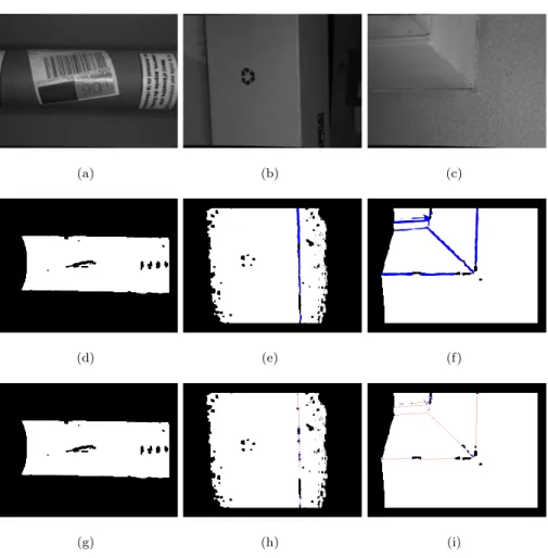
Once the thinning is done, we classify the pixels in the POI region according 155
to three classes : 156
– corners containing the pixels where the median lines intersect in the 157
image ; 158
– sharp features containing the remaining skeleton pixels ; 159
– smooth regions containing the other pixels. 160
Figure 8 depicts several results of classification obtained with this method. 161
This classification of POI pixels will help the subsequent sampling to preserve 162
geometrical features and thus to provide a consistent base mesh in terms of 163
global shape and geometrical characteristics, as explained below. 164
3.3. Coarse sampling 165
This stage is inspired by the feature-preserving Poisson-disk sampling for 166
surfaces of (Peyrot et al., 2015), which is based on a dart throwing. 167
This approach can be efficiently adapted to our setting : the sampling domain 168
Ω becomes the POI region of the stereoscopic images (instead of a surface mesh 169
in (Peyrot et al., 2015)), and the feature lines detected by the previous stage 170
guide the distribution of 2D samples. 171
However, as the output 2D samples of this stage will define the vertices of 172
the base mesh, they must be consistently distributed over the surface of the 173
object (and not especially over its stereoscopic images). Therefore the sampling 174
is done onto the POI region, to benefit from its implicit 2D connectivity, but 175
the distances between samples are computed in the 3D space with Dijkstra’s 176
algorithm (Dijkstra, 1959). 177
The principle of the dart throwing on a 2D image is the following : i) one 178
pixel in the 2D domain Ω is chosen randomly, ii) a disk is computed around 179
it, according to a radius R that depends on the target number N of samples 180
and a density function, iii) this pixel is considered as a valid sample if the disk 181
(a) (b) (c)
(d) (e) (f)
(g) (h) (i)
Figure 8: Detection of the feature lines via our classification technique. First row : left ste-reoscopic images obtained with our scanner (models Pipe, Box and Wall). Second row : detection of high curvature areas (in blue). Third row : resulting classification after thinning : white, red and blue pixels represent respectively the smooth regions, the sharp features and the corners.
does not intersect the disks relative to the samples already accepted (ensuring 182
a minimal distance between the samples). 183
One key idea of the proposed sampling technique is the computation of the 184
radius R onto the surface in the 3D space, while handling the POI region of 185
the stereoscopic images. Given the requested number of samples N , we first 186
calculate the horizontal δi and vertical δj deviations between samples when a
187
uniform sampling pattern is realized on the stereoscopic image. It generates 188
a grid of samples of dimension Nδi × Nδj, as depicted in figure 9, where Ni
189
and Nj represent the number of samples per row and per column, respectively
190 (Ni× Nj= N ). 191 δi δj L H Ni Nj Sample Stereoscopic image
Figure 9: Example of uniform sampling performed on one stereoscopic image.
To take care of the fact that the sampling domain Ω is restricted to the 192
pixels in the POI region, the distances δi and δj between samples along each
193
dimension, are shrunk by a factor Card{P OI}L×H , with Card{P OI} the number of
194
pixels in Ω. A uniform sampling can be realized using 195
R = 1
3 · max(δi, δj) · Sr, (2)
where Sris the spatial resolution of the scanner (0.3mm in our case). With some
196
objects, it can be convenient to realize an adaptive sampling, to better preserve 197
the geometrical features for instance. In that case, the radius will depend on the 198
surface curvature according to the following equation (Peyrot et al., 2015) : 199
R = 1
3 · max(δi, δj) · Sr· (1 + e
C.λ2+ eC.λ3). (3)
Empirically, we put C = −8.0 for the pixels of the class sharp features, and 200
C = −6.0 for the pixels of the class smooth regions. λ2and λ3are the eigenvalues
of the tensor Tp(u,v) computed in section 3.2. In this formulation, the corners
202
pixels keep the minimum radius given by equation (2). To determine the disks 203
associated to the samples in function of the radius R, we recall that we use 204
Dijkstra’s algorithm to compute geodesic distances between 3D points, while 205
using the connectivity of the 2D sampling domain Ω. Therefore, a disk does 206
not depend on the Euclidean distance between two given 2D samples, but on 207
the sum of the lengths of the 3D segments defined by the shortest path in the 208
POI region, as shown in figure 10. As output of this stage, we get a set of 2D 209
samples, that ensures a good distribution of the vertices of the 3D base mesh 210
all over the scanned surface. 211 i j Z X Y 3D geometry 2D connectivity
Figure 10: Computation of a geodesic distance between two points of the surface in R3(right
image), driven by the shortest path between the associated pixels in the POI region (light blue region, left image).
3.4. Semi-regular meshing 212
We now present how to generate a semi-regular mesh directly from the set 213
of 2D samples defined previously. It is a three-stage process : creation of the 3D 214
base mesh from the set of 2D samples, refinement by iterative subdivisions to 215
get a 2D semi-regular mesh, and fitting in 3D space. 216
Creation of the base mesh. The base mesh is obtained via a constrained Voro-217
noi relaxation (Lloyd, 1982) of the samples in the stereoscopic image domain, 218
followed by the triangulation of the relaxed samples (via the dual of the Voronoi 219
diagram (Rong et al.)). In our context, the Voronoi relaxation consists in first 220
computing a Voronoi diagram of the pixels in function of the set of samples, and 221
then displacing each sample to the centroid of its cell. This process is iteratively 222
repeated until convergence. The relaxation greatly improves the mesh quality, 223
when comparing with the triangulation that we could obtain directly from the 224
initial voronoi diagram. 225
In this work, the Voronoi diagrams are generated with (Munshi et al., 2011), 226
that is a GPU implementation of popular Dijkstra’s algorithm (Dijkstra, 1959). 227
We had to adapt this algorithm to process stereoscopic images. Moreover, to 228
preserve the feature lines on the created base mesh, we added a constraint
229
during the relaxation : the new samples must belong to the same class than the 230
initial samples (corners, sharp features or smooth regions). In other words, if 231
after relaxation a sample is moved to a pixel which does not belong to the same 232
class, then the sample is displaced to the closest pixel of the same class. This 233
technique is straightforward, but produces nice triangulations, while preserving 234
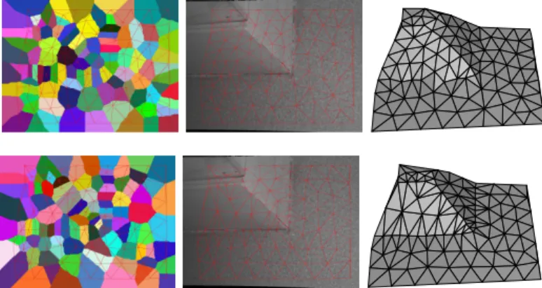
geometrical features of the scanned object, as shown in figure 11. This figure 235
shows also the poor triangulation obtained if the constraint is not included. 236
Figure 11: Base mesh generated by our Voronoi relaxation without (first row) or with (second
row) the constraint on the feature lines. Left : final Voronoi diagram and triangulation.
Middle : the same triangulation on the left stereoscopic image. Right : the resulting 3D base mesh.
Refinement. A 2D semi-regular mesh is first obtained by applying several mid-237
point subdivisions (Chen and Prautzsch, 2012) to the base mesh of the left 238
stereoscopic image (see figure 12). Then, the surface fitting will embed the semi-239
regular mesh in the 3D space. 240
Left stereoscopic image
POI region
(a) (b)
(c) (d)
Figure 12: Generation of the 2D semi-regular mesh. (a) Left stereoscopic image and its POI region ; (b) 2D base mesh ; (c) Subdivision ; (d) Displacement of the new vertices (red ones).
During the subdivision, some new vertices might be either outside the POI 241
region, or in holes (areas without 3D correspondences). In the first case , they 242
are displaced to their closest POI pixel, as shown in figures 12(c) and 12(d). To 243
avoid an exhaustive research over the POI region, we use a parallelized k-Nearest 244
Neighbors algorithm (with k = 1). 245
In the second case, if we use the same technique, the resulting triangles will 246
be badly shaped (see figure 13(a)), which globally decreases the mesh quality. 247
To reduce such artifacts, we choose to keep the vertices ”fallen in a hole” in the 248
2D domain, and so in the 3D space. Figure 13(b) shows that, with this technique, 249
the triangles filling the holes are better shaped. Note that instead of using this 250
simple scheme, one could use an interpolating scheme such as Butterfly (Egli 251
and Dussault, 2001). 252
(a) Without our approximation. (b) With our approximation.
Figure 13: Technique proposed to fill the holes during the refinement.
4. Experimental results 253
4.1. Visual results 254
All our results are generated with a single pair of stereoscopic images ob-255
tained with a hand-held scanning system. Figure 14 gives an overview of our 256
method on the model Face. 257
From the stereoscopic images (a), the POI region (b) is defined, and the base 258
mesh (resolution 0) is created (c). Then, our coarse-to-fine approach generates 259
several resolutions (d, e, f ). At resolution 5, our semi-regular reconstruction, 260
with only 43k vertices, is already a good approximation of the original cloud of 261
250k points given by the stereoscopic system. This is promising in terms of both 262
compactness and compression. Figure 14(g) also shows the textured semi-regular 263
mesh, produced in a very simple way, with one stereoscopic image. No additional 264
texturing technique is necessary as the connectivity of the semi-regular mesh is 265
generated directly on the image domain. This is another great advantage of our 266
approach. 267
4.2. Uniform Vs adaptive sampling 268
We now study the efficiency of our feature-preserving technique, and the 269
difference in terms of triangle quality, between the meshes produced with the 270
uniform/adaptive samplings during the creation of the base mesh (Section 3.3). 271
(a) Left image. (b) POI region. (c) Resolution 0 (50 vertices). (d) Resolution 2 (701 vertices). (e) Resolution 3 (2,745 vertices). (f) Resolution 5 (43,233 vertices). (g) Textured semi-regular mesh. (h) Reference point cloud (249,767 pts).
Figure 14: Semi-regular reconstruction of the model Face.
Figure 15 shows a reconstruction of a surface having sharp features called 273
Door. 274
Subfigures 15(b), (c) and (d) present the results with the uniform sampling, 275
whereas subfigures 15(f ), (g) and h present the results with the adaptive sam-276
pling. We observe on the smooth shadings that the features are globally well 277
preserved whatever the sampling. Some artifacts along them are visible, but 278
they are due to the holes in the POI region that generate notches along features 279
when the base mesh is created (these artifacts would be removed by improving 280
the stereo matching in the scanning system). 281
(a) Left image. (b) Uniform base mesh (300 vertices).
(c) Resolution 2 (4,575 vertices).
(d) Smooth shading.
(e) POI region. (f) Adaptive base
mesh (300 vertices).
(g) Resolution 2 (4,599 vertices).
(h) Smooth shading.
Figure 15: Preservation of the geometrical features of Door, with the uniform or the adaptive sampling.
However, we observe in subfigures 15(b) and (f ) that the adaptive sampling 283
tends to better preserve the features from the lowest resolution. This result was 284
expected, as the adaptive approach takes into account the curvature during the 285
computation of the disks, leading to a dense sampling pattern along the geo-286
metrical features. The counterpart is that the sampling is globally less uniform, 287
and the quality of the triangles is lower : the average minimum angle is 42.5˚ 288
and 37.5˚ respectively for the uniform and the adaptive sampling. 289
290
Figure 16 gives an additional result on Face : we see that the uniform sam-291
pling tends to provide a more isotropic mesh, and that the edges of the base 292
mesh are less visible at high resolutions, which is advocated in case of smooth 293
surfaces. On the database of five objects shown in Figure 17, the uniform sam-294
pling increases of 11% the average min angles. 295
(a) Left image. (b) Uniform base mesh (300 vertices).
(c) Resolution 2 (4,611 vertices).
(d) Smooth shading.
(e) POI region. (f) Adaptive base
mesh (300 vertices).
(g) Resolution 2 (4,629 vertices).
(h) Smooth shading.
Figure 16: Difference of sampling quality obtained on Face in function of uniform/adaptive sampling.
4.3. Runtime 297
We now evaluate the runtime of our semi-regular meshing on five surfaces 298
shown in Figure 17. The results have been obtained with an Intel Core i3 CPU 299
2.30 GHz processor, associated to a 4 GB RAM. 300
(a) Statue (102, 403 points) (b) Face (249, 764 points) (c) House (276, 313 points) (d) Wall (513, 036 points) (e) Door (531, 572 points)
Figure 17: Database used to compute the runtimes of Figure 19.
Figure 18 shows the runtime in function of the resolution, when the base 301
mesh has 50 vertices, and eight resolutions. The inferior part of this figure is a 302
zoom of the graphic, where the Y-axis spans from 0 to 1.
0,0 0,2 0,4 0,6 0,8 1,0 0 1 2 3 4 5 6 7 8 9 10 11 12 13 14 15 16 17 18 0 1 2 3 4 5 6 7 Resolution House Wall Door Statue Face
Figure 18: Runtime in seconds of our method, per resolution. The inferior part is a zoom of the superior one where the Y-axis spans from 0 to 1.
303
As expected, the most ”greedy” resolution is the first one, during which the 304
base mesh is generated (including the Poisson-disk sampling, the constrained 305
2D Voronoi relaxation, and the 2D Delaunay triangulation). The obtaining of 306
the other resolutions is much faster, partly because theses steps have been pa-307
rallelized on GPU. As a proof, the generation of the seventh resolution defined 308
by 705, 281 vertices (528, 768 vertices are added) requires less than 0.6 seconds 309
in the worst case. The higher total runtime to create our semi-regular mesh is 310
around 17 seconds, for the model Door. Nevertheless, this remains very fast. 311
Now, Figure 19 shows the runtime in function of the base mesh density. 312
For each surface, the curve is obtained by averaging the runtime of five tests. 313
Indeed, our algorithm is not deterministic (because of the dart throwing), and 314
the relaxation time depends on the initial sampling. So, we can obtain slightly 315
differences at each resolution for a same surface.
0 5 10 15 20 25 30 50 75 100 150 200 250 300 400
Density of the coarse mesh
House Wall Door Statue Face
Figure 19: Runtimes (in sec.) of our method in function of the number of vertices of the base mesh.
316
We observe the linearity of the total runtime with respect to the number of 317
vertices of the base mesh. The differences between the models is due to the ori-318
ginal point cloud density (ranging from 102, 403 points for Statue to 531, 572 319
points for Door). The curvature of the scanned surface also influences the run-320
time. For instance, Wall contains around 18k points less than Door, but it 321
contains much more pixels classified as sharp features. Finally, the mean sam-322
pling runtime is slower : 5.70 seconds for Wall, while it amounts to 10.90 323
seconds for Door. 324
4.4. Comparison with the classical pipeline 326
We now compare our direct semi-regular meshing with the classical acquisi-327
tion pipeline to get a semi-regular mesh (point cloud generation → triangulation 328
→ semi-regular remeshing). We use a Voronoi-based triangulation technique to 329
generate the original irregular reference mesh Mori from the point cloud
pro-330
vided by our stereoscopic system. This irregular mesh is then remeshed semi-331
regularly either with the SDK SmartMesh based on the patent Fonteles et al. 332
(2014) and developed by the company (Cintoo3D) (a free trial is available on 333
the website), or with Trireme (Guskov, 2007). To our knowledge, they are the 334
only semi-regular remeshing techniques available on the web. Unfortunately, we 335
found out that Trireme is not a suitable tool to remesh our data. Indeed, we 336
could not produce any semi-regular meshes without severe degeneracies and out-337
lier triangles. In the contrary, SmartMesh always provides manifold semi-regular 338
meshes, in particular because it does not use any parameterization, unlike Tri-339
reme. Consequently, we only compare the reconstruction errors and runtimes 340
relative to our semi-regular meshing and to SmartMesh. 341
342
We first compute the symmetric root mean square distance between the 343
set of vertices of our semi-regular meshes, and the set of vertices of Mori (the
344
original point cloud provided by the acquisition system). It permits to assess 345
the fidelity of our sampling to the reference point cloud. The same distance 346
is calculated with the set of vertices of the semi-regular meshes produced by 347
SmartMesh. Figure 20 shows the evolutions of these distances depending on the 348
resolutions : the X-axis indicates the associated number of points. We observe 349
that our method presents lower distances than SmartMesh. It was expected as 350
our method is approximating, contrary to SmartMesh that is interpolating (it 351
optimizes the positions of the vertices such as its semi-regular mesh is close to 352
the reference mesh). Our method has the advantage to determine the majority of 353
vertices among the original point cloud, as the vertices are selected via the pixels 354
of the POI region in the image domain. The only vertices that do not exist in 355
the original point cloud are associated to pixels selected outside the POI region 356
during subdivision. Thus, our method is more accurate when considering only 357
the geometry of the initial surface.
0,02500 0,03000 0,03500 0,04000 Wall 0,00000 0,00500 0,01000 0,01500 0,02000 100 1000 10000 100000 1000000 SmartMesh Our method (a) Wall 0,01500 0,02000 0,02500 Door 0,00000 0,00500 0,01000 100 1000 10000 100000 1000000 SmartMesh Our method (b) Door 0 02000 0,02500 0,03000 0,03500 Statue 0,00000 0,00500 0,01000 0,01500 0,02000 10 100 1000 10000 100000 SmartMesh Our method (c) Statue 0 02000 0,02500 0,03000 0,03500 Face 0,00000 0,00500 0,01000 0,01500 0,02000 100 1000 10000 100000 1000000 SmartMesh Our method (d) Face
Figure 20: Comparison of the geometry sampling obtained with our method and with Smart-Mesh (Cintoo3D), depending on the vertex density of the semi-regular meshes.
358
We now assess the fidelity of our semi-regular meshes with respect to the 359
reference mesh Mori. To achieve this goal, we compute the symmetric Root
360
Mean Square (RMS) distance between Mori and our semi-regular meshes Msr
361
(normalized by the diagonal length of the bounding box), which is widespread 362
used in the state-of-the-art (Payan et al., 2015). However, in our context, this 363
measure is not suited. Indeed, as explained in section 3.4, our method fills the 364
holes, in order to make the texturing easier and to enhance the mesh quality. 365
As a consequence, when measuring the symmetric RMS distances between our 366
semi-regular meshes and the reference irregular mesh Mori, the distances
bet-367
ween the triangles filling the holes and the original surface are inevitably high. 368
It severely corrupts the comparison with SmartMesh, as this latter has been ini-369
tially developed to preserve the potential borders of a surface and consequently 370
the holes. So, to make fairly comparisons, we compute the asymmetric RMS 371
distance RM S(Mori → Msr), which excludes the filled holes : see Figure 21
372
(the X-axis still indicates the number of points of each resolution). Globally, we 373
observe that our method is better than SmartMesh in the first resolutions. It 374
can be explained by the fact that our method tends to preserve the geometrical 375
features in the base mesh, and that it is approximating (Payan et al., 2015). On 376
the other hand, SmartMesh becomes better on the highest resolutions, because 377
it minimizes the geometric distortion directly onto the original surface, without 378
any parameterization, which avoids the relative distortion. Furthermore, our 379
method is penalized by the fact that it works in the image domain, but also by 380
our feature preservation that positions more vertices on them. 381 382 0 00400 0,00500 0,00600 0,00700 h d 0,00000 0,00100 0,00200 0,00300 0,00400 100 1000 10000 100000 1000000 Our method SmartMesh (a) Wall 0 00200 0,00250 0,00300 0,00350 h d 0,00000 0,00050 0,00100 0,00150 0,00200 100 1000 10000 100000 1000000 Our method SmartMesh (b) Door 0,00800 0,01000 0,01200 h d 0,00000 0,00200 0,00400 0,00600 10 100 1000 10000 100000 Our method SmartMesh (c) Statue 0,00400 0,00500 0,00600 h d 0,00000 0,00100 0,00200 0,00300 100 1000 10000 100000 1000000 Our method SmartMesh (d) Face
Figure 21: addAsymmetric RMS distance RM S(Mori → Msr) obtained with our method
and with SmartMesh (Cintoo3D) in function of the resolution.
On the other hand, our algorithm is direct and thus significantly faster than 383
SmartMesh. The runtime comparison is summarized in table 1. SmartMesh in-384
deed takes several minutes to produce the semi-regular meshes : from 2 to 7 385
minutes in function of the data, excluding the triangulation time, whereas our 386
method needs always less than one minute. Finally, it shows that the proposed 387
pipeline is a promising alternative to the classical one.
Models Wall Door Statue Face
Base mesh density 431 800 365 492
SmartMesh ≥3 min. ≥ 7 min. ≥ 2 min. ≥ 6min.
Our method 19.1 sec. 27.7 sec. 10.1 sec. 10.3 sec.
Table 1: Runtime comparison in seconds between our method and SmartMesh (Cintoo3D), to generate 5 resolutions.
388
5. Conclusion and perspectives 389
In this paper we proposed an alternative to the fastidious pipeline to get 390
semi-regular meshes from physical objects. The idea is to generate semi-regular 391
meshes directly from the stereoscopic images acquired with a hand-held stereo 392
acquisition system. The key idea of our work is that the stereoscopic images 393
can be considered as a parameterization of the acquired surface. Therefore, our 394
reconstruction method processes the data as much as possible into the image 395
domain, before embedding the surface in the 3D space. 396
The first contribution is an original sampling that creates a base mesh of the 397
scanned surface. We show that the Poisson-disk sampling developed by (Peyrot 398
et al., 2013) can be extended to a stereoscopic system, while retrieving the 3D 399
information necessary to preserve features all along the process. This allows to 400
take into account the surface geometry, although the sampling is realized on 401
the stereoscopic images. The second contribution concerns our coarse-to-fine 402
approach that allows to get a semi-regular mesh preserving the geometrical 403
features as output of our acquisition system, by working mainly in the image 404
domain. 405
Our pipeline could be easily included into any stereoscopic acquisition sys-406
tem. It also has the advantage to create semi-regular output that can be directly 407
textured with the stereoscopic image, and is also much more faster and conve-408
nient than the classical pipeline. 409
However, a lot of improvements remains possible. For instance, the runtime 410
of our algorithm can be improved as some parts are implemented on CPU. 411
It would be interesting to investigate parallel algorithms for all the stages, to 412
allow quasi real-time reconstructions. We could also investigate new means to 413
improve the shape fidelity, in order to be competitive with the semi-regular 414
remeshing techniques. Another promising improvement would be to manage 415
several views. Indeed, our current algorithm handles only one view, and thus 416
only a part of the scanned object can be reconstructed. It would be relevant 417
to study, for instance, mosaicing techniques, widespread in photogrammetry, to 418
generate a large POI region representing the whole parameterized object, and 419
thus to output a complete semi-regular representation of a physical object. 420
421
Acknowledgements This work was supported by a grant from R´egion
Pro-422
vence Alpes Cˆote d’Azur in France.
423
Bibliography 424
425
Q. Chen and H. Prautzsch. General midpoint subdivision. CoRR,
426
abs/1208.3794, 2012. 427
Cintoo3D. SDK smartmesh. http://www.cintoo3D.com. 428
E. W. Dijkstra. A note on two problems in connexion with graphs. Numerische 429
Mathematik, 1 :269–271, 1959. 430
R. Egli and J.-P. Dussault, editors. Technique butterfly g´en´eralis´ee, Dijon,
431
France, p. 133-136, 2001. Actes de Compression et Repr´esentation des
Si-432
gnaux Audiovisuels. 433
L. Hidd Fonteles, A. Meftah, M. Antonini, and F. Payan. Method, system and 434
computer program product for 3d objects graphical representation. FR-13, n 435
4152728.3-1502, 2014, CNRS et Universit de Nice - Sophia Antipolis, 2014. 436
I. Guskov. Manifold-based approach to semi-regular remeshing. Graphical Mo-437
dels, 69(1) :1–18, 2007. 438
R. I. Hartley and A. Zisserman. Multiple View Geometry in Computer Vision. 439
Cambridge University Press, second edition, 2004. 440
E. C. Hernandez, G. Vogiatzis, and R. Cipolla. Multiview photometric stereo. 441
IEEE Trans. Pattern Anal. Mach. Intell., 30(3), March 2008. 442
S. P. Lloyd. Least squares quantization in pcm. IEEE Transactions on Infor-443
mation Theory, 28 :129–137, 1982. 444
M. Lounsbery, T. D. DeRose, and J. Warren. Multiresolution analysis for sur-445
faces of arbitrary topological type. ACM Trans. Graph., 16(1), January 1997. 446
A. Munshi, B.-R. Gaster, T.-G. Mattson, J. Fung, and D. Ginsburg. OpenCL 447
Programming Guide. Prentice Hall, 2011. 448
J. Park, S. N. Sinha, Y. Matsushita, Y.-W. Tai, and I. S. Kweon. Multiview 449
photometric stereo using planar mesh parameterization. Computer Vision, 450
IEEE International Conference on, 0, a. 451
M. K. Park, S. J. Lee, and K. H. Lee. b. 452
F. Payan and M. Antonini. Mean square error approximation for wavelet-based 453
semiregular mesh compression. Transactions on Visualization and Computer 454
Graphics (TVCG), 12, 2006. 455
F. Payan, C. Roudet, and B. Sauvage. Semi-regular triangle remeshing : a
456
comprehensive study. Computer Graphics Forum, 34 :86–102, February 2015. 457
J.-L. Peyrot, F. Payan, and M. Antonini. Feature-preserving Direct Blue Noise 458
Sampling for Surface Meshes. In Eurographics (Short Papers), pages 9–12, 459
2013. 460
J.-L. Peyrot, F. Payan, N. Ruchaud, and M. Antonini. Stereo reconstruction of 461
semiregular meshes, and multiresolution analysis for automatic detection of 462
dents on surfaces. In Proceedings of IEEE International Conference in Image 463
Processing (ICIP), Paris, France, october 2014. 464
J.-L. Peyrot, F. Payan, and M. Antonini. Direct blue noise resampling of meshes 465
of arbitrary topology. The Visual Computer, 31 :1365–1381, september 2015. 466
N. Pietroni, M. Tarini, O. Sorkine, and D. Zorin. Global parametrization of 467
range image sets. ACM Trans. Graph., 30(6), December 2011. 468
G. Rong, T.-S. Tan, T.-T. Cao, and Stephanus. In Eric Haines and Morgan 469
McGuire, editors, SI3D. 470
D. Scharstein and R. Szeliski. A taxonomy and evaluation of dense two-frame 471
stereo correspondence algorithms. Int. J. Comput. Vision, 47(1-3) :7–42, April 472
2002. ISSN 0920-5691. 473
S. M. Seitz, B. Curless, J. Diebel, D. Scharstein, and R. Szeliski. A comparison 474
and evaluation of multi-view stereo reconstruction algorithms. In Proceedings 475
of the 2006 IEEE Computer Society Conference on Computer Vision and 476
Pattern Recognition - Volume 1, CVPR ’06, 2006. 477
N. Snavely, S. M. Seitz, and R. Szeliski. Photo tourism : Exploring photo
478
collections in 3d. ACM Trans. Graph., 25(3) :835–846, July 2006. 479
T. Y. Zhang and C. Y. Suen. A fast parallel algorithm for thinning digital 480
patterns. Commun. ACM, 27(3), March 1984. 481
K. Zhou, J. Synder, B. Guo, and H.-Y. Shum. Iso-charts : Stretch-driven mesh 482
parameterization using spectral analysis. Eurographics, July 2004. 483