Chaotic Pseudo Random Number Generators via Ultra Weak Coupling of Chaotic Maps and Double Threshold Sampling Sequences

HAL Id: hal-00386292

https://hal.archives-ouvertes.fr/hal-00386292

Submitted on 20 May 2009

HAL is a multi-disciplinary open access

archive for the deposit and dissemination of

sci-entific research documents, whether they are

pub-lished or not. The documents may come from

teaching and research institutions in France or

abroad, or from public or private research centers.

L’archive ouverte pluridisciplinaire HAL, est

destinée au dépôt et à la diffusion de documents

scientifiques de niveau recherche, publiés ou non,

émanant des établissements d’enseignement et de

recherche français ou étrangers, des laboratoires

publics ou privés.

Weak Coupling of Chaotic Maps and Double Threshold

Sampling Sequences

René Lozi

To cite this version:

René Lozi. Chaotic Pseudo Random Number Generators via Ultra Weak Coupling of Chaotic Maps

and Double Threshold Sampling Sequences. ICCSA 2009, 3rd Conference on Complex Systems and

Applications., Jun 2009, Le Havre, France. pp.20-24. �hal-00386292�

University of Le Havre, France, June 29- July 02, 2009.

Abstract—Generation of random or pseudorandom numbers, nowadays, is a key feature of industrial mathematics. Pseudorandom or chaotic numbers are used in many areas of contemporary technology such as modern communication systems and engineering applications. More and more European or US patents using discrete mappings for this purpose are obtained by researchers of discrete dynamical systems [1], [2]. Efficient Chaotic Pseudo Random Number Generators (CPRNG) have been recently introduced. They use the ultra weak multidimensional coupling of p 1-dimensional dynamical systems which preserve the chaotic properties of the continuous models in numerical experiments. Together with chaotic sampling and mixing processes, ultra weak coupling leads to families of (CPRNG) which are noteworthy [3], [4].

In this paper we improve again these families using a double threshold chaotic sampling instead of a single one.

We analyze numerically the properties of these new families and underline their very high qualities and usefulness as CPRNG when very long series are computed.

Index Terms—Chaos, Discrete time systems, Floating point arithmetic, Random number generation.

I. INTRODUCTION

Efficient Chaotic Pseudo Random Number Generators (CPRNG) have been recently introduced. The idea of applying discrete chaotic dynamical systems, intrinsically, exploits the property of extreme sensitivity of trajectories to small changes of initial conditions. They use the ultra weak multidimensional coupling of p 1-dimensional dynamical systems which preserve the chaotic properties of the continuous models in numerical experiments. The process of chaotic sampling and mixing of chaotic sequences, which is pivotal for these families, works perfectly in numerical simulation when floating point (or double precision) numbers are handled by a computer.

It is noteworthy that these families of very weakly coupled maps are more powerful than the usual formulas used to generate chaotic sequences mainly because only additions and

R. Lozi is with the Laboratory J. A. Dieudonné, UMR CNRS 6621, University of Nice Sophia-Antipolis, 06108 Nice Cedex 02, France and the Institut Universitaire de Formation des Maîtres Célestin Freinet-académie de Nice, University of Nice-Sophia-Antipolis, 89 avenue George V, 06046 Nice Cedex 1, France (corresponding author to provide phone: 04-93-53-75-08; e-mailrlozi@unice.fr).

multiplications are used in the computation process; no division being required. Moreover the computations are done using floating point or double precision numbers, allowing the use of the powerful Floating Point Unit (FPU) of the modern microprocessors (built by both Intel and Advanced Micro Devices (AMD)). In addition, a large part of the computations can be parallelized taking advantage of the multicore microprocessors which appear on the market of laptop computers.

In this paper we improve the properties of these families using a double threshold chaotic sampling instead of a single one. The genuine map f used as one-dimensional dynamical systems to generate them is henceforth perfectly hidden.

II. ULTRA WEAK MULTIDIMENSIONAL COUPLING

A. System of p-Coupled Symmetric Tent Map

When a dynamical system is realized on a computer using floating point or double precision numbers, the computation is of a discretization, where finite machine arithmetic replaces continuum state space. For chaotic dynamical systems, the discretization often has collapsing effects to a fixed point or to short cycles [5], [6]. In order to preserve the chaotic properties of the continuous models in numerical experiments we have recently introduced an ultra weak multidimensional coupling of

p one-dimensional dynamical systems which is noteworthy [7].

In this specific case we have chosen as an example the symmetric tent map defined by

x a x

fa( )=1− (1)

with the value a = 2, later denoted simply as f, even though others chaotic map of the interval (as the logistic map) can be used for the same purpose. The dynamical system associated to this one dimensional map is defined by the equation on the interval J = [-1, 1]⊂ℝ [8].

n

n ax

x₊1=1− (2)

The system of p-coupled dynamical systems is then:

( )

n

(

( n)

)

1

n F X A f X

X ₊ = = ⋅ (3)

with

Chaotic Pseudo Random Number Generators via

Ultra Weak Coupling of Chaotic Maps and

Double Threshold Sampling Sequences.

          = p x x X ⋮ 1 ,           = ) ( ) ( ) ( 1 p x f x f X f ⋮ (4) and                 = p p p 2 2 2 2 1 1 1 1 ε 1) -(p -1 ε ε ε ε ε 1) -(p -1 ε ε ε ε ε 1) -(p -1 ⋯ ⋯ ⋮ ⋮ ⋱ ⋮ ⋮ ⋮ ⋱ ⋮ ⋯ ⋯ A (5)

F is a map of Jp into itself.

Several combinations can be given for the relative values of the

i

ε, in this paper we choose

1

i ε

ε =_i i = 2, …, p (6)

The matrix A is always a stochastic matrix iff the coupling constants ε_i verify i 1 0 ε 1 p ≤ ≤ − (7)

When ε_i=₀ the maps are decoupled, when

i 1 ε 1 p = − they

are fully cross coupled. Generally, researchers do not consider very small values of ε_i because it seems that the maps are quasi

decoupled with those values and no special effect of the coupling is expected. In fact it is not the case and ultra small coupling constant (as small as 10-7 for floating point numbers or 10-14 for double precision numbers), allows the construction of very long periodic orbits, leading to sterling chaotic generators. Moreover each component of these numbers belonging to p

ℝ is equally distributed over the finite interval J ⊂ℝ . Numerical computations show that this distribution is obtained with a very good approximation. They have also the property that the length of the periods of the numerically observed orbits is very large [7].

B. Chaotic Pseudo-Random Generators

However chaotic numbers are not pseudo-random numbers because the plot of the couples of iterated points (xn, xn+1) in the phase plane reveals the map f used as one-dimensional dynamical systems to generate them.

Nevertheless we have recently introduced a family of Enhanced Chaotic Pseudo Random Number Generators (CPRNG) in order to compute very fast long series of pseudorandom numbers with desktop computer [9]. This family is based on the previous ultra weak coupling which is enhanced in order to conceal the chaotic genuine function.

In the aim of hiding f in the phase space

(

l

)

n l n x

x , +1 two

mechanisms are used. The pivotal idea of the first one mechanism is to sample chaotically the sequence

(

0, 1, 2,…, , 1,…

)

l n l n l l l x x x x

x + generated by the l-th component l x , selecting l

n

x every time the value m n

x of the m-th component m

x , is strictly greater than a threshold T ∈ J, with l ≠ m, for 1 ≤ l, m ≤ p .

A second mechanism can improve the unpredictability of the chaotic sequence generated as above, using synergistically all the components of the vector X, instead of two. This simple mechanism is based on the chaotic mixing of the p-1 sequences

(

, , ,…, , 11,…

)

1 1 2 1 1 1 0 x x xn xn+ x ,

(

, , ,…, , 21,…

)

2 2 2 2 1 2 0 x x xn xn+ x ,…,

(

, , ,…, , 1,…

)

1 1 1 2 1 1 1 0 − + − − − − p n p n p p p x x x x

x using the last one

(

0, 1, 2,…, , 1,…

)

p n p n p p p x x x x

x + with respect to a given partition T1,

T2, …, Tp-1 of J, to distribute the iterated points.

C. Numerical Results

As an example we explicit both mechanisms taking

4-coupled equations for (3). The value of 4

n

x commands the chaotic sampling and the mixing processes as follows.

Let us set three threshold values T1, T2 and T3 -1 < T1 < T2 < T3 < 1 (8)

we sample and mix together chaotically the sequences

(

, , ,…, , 11,…

)

1 1 2 1 1 1 0 x x xn xn+ x ,

(

, , ,…, , 2 ,…

)

1 2 2 2 2 1 2 0 x x xn xn+ x and

(

, , ,…, , 3 ,…

)

1 3 3 2 3 1 3 0 x x xn xn+ x defining

(

x₀,x₁,x₂,⋯,x_q,x_q+1,⋯

)

by

]

[

[

[

[

[

     ∈ ∈ ∈ = 1 , , , 3 4 3 3 2 4 2 2 1 4 1 T x iff x T T x iff x T T x iff x x n n n n n n q (9)

Numerical results about chaotic numbers produced by (3) - (9) show that they are equally distributed over the interval J.

In order to compute numerically an approximation of the invariant measure also called the probability distribution function PN (x) linked to the 1-dimensional map f we consider a

regular partition of M small intervals (boxes) ri of J.

J= 1 0 M i r −

∪

(10) ri = [si , si+1[ , i = 0, M – 2 (11) rM-1 = [sM-1 , 1] (12) M i si 2 1+ − = i = 0, M (13) the length of each box is

M s si i 2 1− = + (14)

All iterates f (n)(x) belonging to these boxes are collected (after a transient regime of Q iterations decided a priori, i.e. the first Q iterates are neglected). Once the computation of N+ Q iterates is completed, the relative number of iterates with respect to N/M in each box ri represents the value PN (si). The approximated PN (x) defined in this article is then a step

function, with M steps. As M may vary, we define

( )

i i N M r N M s P # 2 1 ) ( , = (15)

where #ri is the number of iterates belonging to the interval ri and the constant 1/2 allows the normalisation of PM,N(x) on the

interval J. i i N M N M x P s x r P , ( )= , ( ) ∀ ∈ (16)

University of Le Havre, France, June 29- July 02, 2009. In the case of coupled maps, we are more interested by the distribution of each component x1, …, xp of X rather than the distribution of the variable X itself in Jp. We then consider the approximated probability distribution function PN(xj) associated

to one among several components of F(X) defined by (3) which are one-dimensional maps.

The discrepancies E1 (in norm L1) and E2 (in norm L2)

between PN_disc,N_iter(x) and the Lebesgue measure which is the

invariant measure associated to the symmetric tent map, are defined by 1 5 . 0 ) ( ) , ( _, 1 Ndisc Niter PN N x _L E iter disc − = (17) 2

2( disc, iter) Ndisc,Niter( ) 0.5 L

E N N = P x − (18)

In the same way an approximation of the correlation distribution function CN (x, y) is to obtained numerically

building a regular partition of M 2 small squares (boxes) of J2 imbedded in the phase subspace (xl, xm)

ri,j = [si , si+1[ × [tj , tj+1[ , i, j = 0, M – 2 (19) rM-1,j = [sM-1 , 1] × [tj , tj+1[ , j = 0, M – 2 (20) ri,M-1 = [si , si+1[× [tM-1 , 1] , i = 0, M – 2 (21) rM-1,M-1 = [sM-1 , 1] × [tM-1 , 1] (22) M i si 2 1+ − = , M j tj 2 1+ − = , i, j = 0, M (23)

the measure of the area of each box is

(

1

) (

1

)

2 2       = − ⋅ − ₊ + M t t s si i i i (24)

Once N + Q iterated points

(

m

)

n l n x

x , belonging to these boxes

are collected the relative number of iterates with respect to

N/M2 in each box ri,j represents the value CN (si,tj). The approximated probability distribution function CN (x,y) defined

here is then a 2-dimensional step function, with M 2 steps. As M can take several values in the next sections, we define

( )

ij j i N M r N M t s C , 2 , # 4 1 ) , ( = (25)

where #ri,j is the number of iterates belonging to the square ri,j and the constant 1/4 allows the normalisation of _CM,N(x,y) on the square J2. j i j i N M N M x y C s t x y r C , ( , )= , ( , ) ∀( , )∈ , (26) The discrepancies 1 C

E

in norm L1 between CNdisc,Niter(x,y) and the uniform distribution on the square is defined by

1 1 , ( , ) _{disc iter}( , ) 0.25 C disc iter N N _L E N N = C x y − (27)

Finally letACM,N(x,y) be the autocorrelation distribution function which is the correlation function CM,N(x,y) of (26)

defined in the phase space

(

l

)

n l n x

x , +1 instead of the phase space

(xl, xm). In order to control that the enhanced chaotic numbers

(

x0,x1,x2,⋯,xq,xq+1,⋯

)

are uncorrelated, we plot them in the phase subspace

(

xn,xn₊₁

)

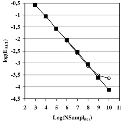
and we check if they are uniformly distributed in the square J2 and if f is concealed .

Fig. 1 shows the values of EAC1(Ndisc,NSampliter) for a system of 4-coupled equations when the three components

x1 , x2 , x3 are mixed and sampled by x4 for the threshold values

T1 = 0.98, T2 = 0.987, T3 = 0.994 or T1 = 0.998, T2 = 0.9987, T3 = 0.9994. -4,5 -4 -3,5 -3 -2,5 -2 -1,5 -1 -0,5 2 3 4 5 6 7 8 9 10 11 Log(NSamplite r) lo g (E A C 1 ) Thresholds 0,98 ; 0,987; 0,994 Thresholds 0,998 ; 0,9987; 0,9994 Figure 1. Error of 1( , ) AC disc iter E N NSampl Ndisc=102×102, NSampliter= 103 to 1010, εi = i.ε1, ε1=10-14.

Niter NSampliter

1( , ) AC disc iter E N NSampl 4-coupled equation T1 = 0.998, T2 = 0.9987, T3 = 0.9994 105 93 0.68924731 106 1015 0.25881773 107 10,139 0.086706776 108 100,465 0.026815309 109 1,000,549 0.0089111078 1010 9,998,814 0.0027932033 1011 100,001,892 0.00085967214 1012 999,945,728 0.0002346851 1013 10,000,046,137 0.000073234736 Table 1. Error of 1( , ) AC disc iter

E N NSampl for a system of 4 coupled-equations when the three components x1 , x2 , x3 are mixed and sampled by x4 for the threshold values T1 = 0.998,

III. DOUBLE TRHESHOLD CHAOTIC SAMPLING

A. Improved CPRNG

On can again improve the CPRG previously introduced with respect to the infinity norm instead of the L1 or L2 norms because the _L∞norm is more sensitive than the others to reveal the concealed f. For this aim, consider first that in the phase space

(

)

l n l n x

x , +1 _{the graph of the chaotically sampled chaotic}

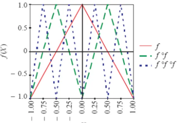
numbers is a mix of the graphs of all the f (r) (Fig. 2).

It is obvious as showed on Fig. 3 that for r = 1 if M = 1 or 2,

, ( , )

M N

AC x y is constant and normalized on the square hence

1 2

( , ) ( , ) ( , ) 0

AC AC AC

E _∞ M N =E M N =E M N = .

The autocorrelation function is different from zero only if M > 2 (Fig. 4).

Figure 2. Graphs of the symmetric tent map f, f (2) and f (3) on the interval [-1,1].

Figure 3. In shaded regions the autocorrelation distribution , ( , )

M N

AC x y is constant for the symmetric tent map f on the

interval [-1, 1] for M = 1 or 2.

In the same way as displayed on Fig. 5, 6 and 7,

1 2

( , ) ( , ) ( , ) 0

AC AC AC

E ∞ M N =E M N =E M N = for f

(i) _{iff M < 2}i_. Hence for a given M, if we cancel the contribution of all the f (i) for 2i < M, it is not possible to identify the genuine function f.

Figure 4. Regions where the autocorrelation distribution , ( , )

M N

AC x y is constant for the symmetric tent map f are shaded,

for M = 4. (The square on the bottom left of the graph shows the size of the ri,j box). ACM N, ( , )x y vanishes on the white regions.

Figure 5. In shaded regions the autocorrelation distribution , ( , )

M N

AC x y is constant for the symmetric tent map f (2) on the interval [-1, 1] for M = 1, 2 and 4.

Figure 6. Regions where the autocorrelation distribution , ( , )

M N

AC x y is constant for the symmetric tent map f (2) are shaded for M = 8.

B. Algorithm and Numerical Results

We describe again the algorithm of the double threshold chaotic sampling in the case of 4-coupled equations.

Consider the sequence

(

x0,x1,x2,⋯,xq,xq+1,⋯

)

we want to mix

and sample. For each q-1 there exists n(q-1) in the original sequence. We introduce a second threshold

N

'

∈

ℕ

and then we define:

]

[

[

[

[

[

1 4 1 2 ( 1) 2 4 2 3 ( 1) 3 4 3 ( 1) , ' , ' , 1 ' n n q q n n q n n q x iff x T T and n n N x x iff x T T and n n N x iff x T and n n N − − −  _{∈ − >}  = ∈ − >  _{∈ − >}  (28)

University of Le Havre, France, June 29- July 02, 2009.

Figure 7. Regions where the autocorrelation distribution , ( , )

M N

AC x y is constant for the symmetric tent map f (3) are

shaded for M = 16.

As shown previously [9] the errors in L1 or L2 norms decrease with the number of chaotic points (as in the law of large numbers) and conversely increase with the number M of boxes used to define ACM N_, ( , )x y . It is the same for the error in

L

∞ norm. Fig. 8 shows that when M is greater than 25, the sequence defined by (28) behaves better than the one defined by (9).

Figure 8. Error of EAC∞(Ndisc,NSampliter) Ndisc= 2 1 _{to 2}10_,

NSampliter = 109, thresholds T = 0.9 and N’ = 20, εi = i.ε1,

ε1 = 10-14.

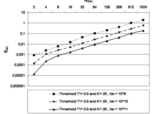
Fig. 9 shows that when the number of chaotic points increases the error

L

_∞decreases drastically. If N’ > 100, it is necessary to use a huge grid of 2100x2100 boxes splitting the square J2 in order

to find a trace of the genuine function f. This is numerically impossible with double precision numbers. Then the chaotic numbers appear as random numbers.

Others numerical results show the high-potency of theses new CPRNG. Due to limitation of this article, they will be published elsewhere.

IV. CONCLUSION

Using a double threshold in order to sample a chaotic sequence, we have improved with respect to the infinity norm the CPRNG previously introduced. When the value of the

second threshold N’ is greater than 100, it is impossible to find the genuine function used to generate the chaotic numbers. The new CPRNG family is robust versus the choice of the weak parameter of the system for 10-14 < ε < 10-5, allowing the use of this family in several applications as for example chaotic cryptography.

Figure 9. Error of EAC∞(Ndisc,NSampliter) Ndisc= 2

1 _{to 2}10_,

NSampliter = 109 to 1011, thresholds T = 0.9 and N’ = 20,

εi = i.ε1, ε1 = 10-14.

REFERENCES

[1] Petersen, M. V., Sorensen, H. M., Method of generating pseudo-random numbers in an electronic device, and a method of encrypting and decrypting electronic data. United States Patent 7170997, 2007.

[2] Ruggiero, D., Mascolo, D., Pedaci, I., Amato, P., Method of generating successions of pseudo-random bits or numbers. United States Patent

Application 20060251250, 2006.

[3] S. Hénaff, I. Taralova, R. Lozi, Observers design for a new weakly coupled map function, preprint. http://hal.archives-ouvertes.fr/hal-00368576/fr/ [4] S. Hénaff, I. Taralova, R. Lozi, Dynamical Analysis of a new statistically highly performant deterministic function for chaotic signals generation, preprint. http://hal.archives-ouvertes.fr/hal-00368844/fr/

[5] O. E., Lanford III, Some informal remarks on the orbit structure of discrete approximations to chaotic maps. Experimental Mathematics, Vol. 7, 4, 317-324, 1998.

[6] Gora, P., Boyarsky, A., Islam, Md. S., Bahsoun, W., Absolutely continuous invariant measures that cannot be observed experimentally. SIAM J. Appl. Dyn.

Syst., 5:1, 84-90 (electronic), 2006.

[7] Lozi, R., Giga-Periodic Orbits for Weakly Coupled Tent and Logistic Discretized Maps. International Conference on Industrial and Applied Mathematics, New Delhi, december 2004, Modern Mathematical Models,

Methods and Algorithms for Real World Systems, A.H. Siddiqi, I.S. Duff and

O. Christensen (Editors), Anamaya Publishers, New Delhi, India pp. 80-124, 2006.

[8] Sprott, J. C., Chaos and Time-Series Analysis. Oxford University Press, Oxford, UK, 2003.

[9] R. Lozi, New Enhanced Chaotic Number Generators, Indian Journal of