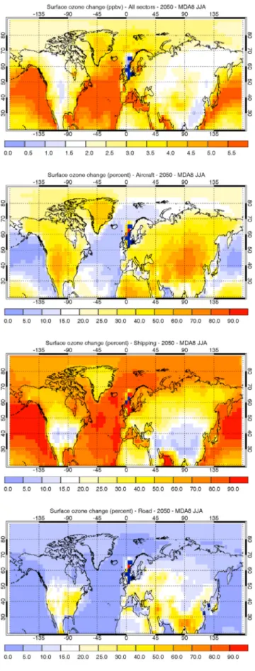
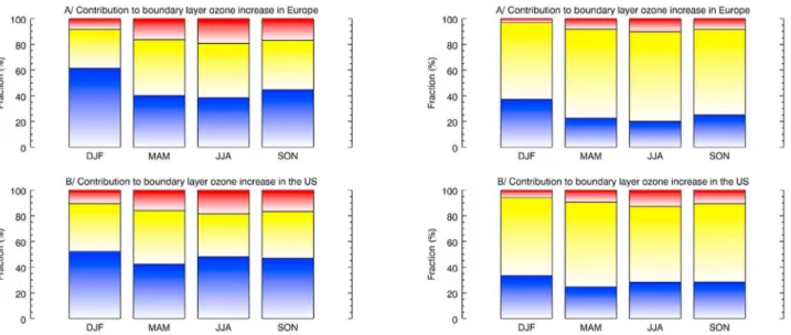
Boundary layer ozone pollution caused by future aircraft emissions
Texte intégral
Figure
Documents relatifs
In this paper, four methods of measuring sensitivity, the field vane, the unconfined compressio~l test, the laboratory vane, and the fall-cone test are
Pour prédire les efforts transmis au châssis, le modèle et le terme source, tous deux décrits dans la relation (5), sont requis.. Or, le terme source est présentement
Une étude plus spécifique de la source 1308+326 a montré que la trajectoire de la composante VLBI notée 1 (qui est l’une des deux composantes utilisées pour modéliser la structure
Sur le bassin versant de l’Héraut (fig. 62)., le rapport Sr/Ca est proche de 1.5‰ dans le domaine du socle puis décroît à l’entrée du domaine karstique pour se stabiliser
Elle substitue à l’idée d’une coordination des activités par une division du travail celle qui vise une coordination des interactions par les objets (Bowker et
Les travaux de [Limido, 2008] reprennent cette approche mais cette fois-ci plusieurs profils de rugosité sont extraits d’une surface 3D simulée (par approche Z-map). Cette
An architectural and topological design tool is developed to enable the high-level analysis and optimization of sensor architectures targeted to a particular set
