Design, construction, and analysis of a modular ship model and open-source autonomous surface vehicle

Design, Construction, and Analysis of a Modular

Ship Model and Open-Source Autonomous Surface

Vehicle

by

Austin Jolley

Submitted to the Department of Mechanical Engineering

in partial fulfillment of the requirements for the degrees of

Naval Engineer

and

Master of Science in Mechanical Engineering

at the

MASSACHUSETTS INSTITUTE OF TECHNOLOGY

May 2020

c

○ Austin Jolley, MMXX. All rights reserved.

The author hereby grants to MIT permission to reproduce and to

distribute publicly paper and electronic copies of this thesis document

in whole or in part in any medium now known or hereafter created.

Author . . . .

Department of Mechanical Engineering

May 8, 2020

Certified by . . . .

Alexandra H. Techet

Professor of Mechanical and Ocean Engineering

Thesis Supervisor

Accepted by . . . .

Nicolas Hadjiconstantinou

Chairman, Department Committee on Graduate Theses

Design, Construction, and Analysis of a Modular Ship Model

and Open-Source Autonomous Surface Vehicle

by

Austin Jolley

Submitted to the Department of Mechanical Engineering on May 8, 2020, in partial fulfillment of the

requirements for the degrees of Naval Engineer

and

Master of Science in Mechanical Engineering

Abstract

Existing models used to explore hydrostatic, hydrodynamic, seakeeping, and maneu-vering characteristics of ships are limited in that their characteristics are essentially static. The effects of various hull appendages, propulsion configurations, and bow and stern designs are difficult to quantify without procuring, instrumenting, and testing entirely new hullform models. Additionally, the realm of marine autonomy has opened up new avenues for exploration in naval architecture which favor endurance and econ-omy over more traditional design goals of speed and capacity. This creates a need for a framework to rapidly design and prototype unmanned surface vessels. This thesis explores the design, manufacture, and analysis of an additively manufactured mod-ular ship model. This model allows for easily altering the shape of the bow and/or stern and it can be lengthened or shortened by the addition or removal of parallel midbody modules. Other designed modules allow the model to be connected to a towing carriage for captive model testing, or be powered and controlled remotely or autonomously for free-running model testing or use as a small Autonomous Surface Vehicle. Analysis of various combinations of these modules was conducted and the results are presented. Additionally, select experiments and design analyses have been developed for educational use as laboratory experiments or academic projects with the goal of furthering the teaching of naval architecture and marine engineering. Thesis Supervisor: Alexandra H. Techet

Acknowledgments

First and foremost, I would like to thank my wife, Nicole, for her years of selfless devotion and sacrifice. This would not have been possible without her. I would also like to express my gratitude towards Professor Alexandra Techet for providing the freedom, flexibility, and necessary counsel to work on this project. I am equally indebted to the Naval Construction and Engineering Program at MIT and the United States Navy for providing the opportunity and support to continue my education at such a prestigious institution. Likewise, I would like to express my gratitude towards my parents for instilling in me a lifelong eagerness to learn and for supporting me in all of my endeavours.

Finally, I would like to dedicate this work to my lovable children, Mackenzie, Gabriel, and Genevieve, and I would like to thank them for providing a challenging environment in which to test my perseverance, patience, and resolve. It would not have been the same without them and the joy they bring to my life.

Contents

1 Introduction/Background 13

1.1 Motivation/Design Philosophy and Requirements . . . 14

1.2 Naval Architecture Theory . . . 15

1.2.1 Principal Dimensions . . . 16

1.2.2 Coefficients of Form . . . 18

1.2.3 Hydrostatics and Stability . . . 19

1.3 Project Overview . . . 20

2 Design and Construction 21 2.1 Monohull Design . . . 21

2.1.1 Principal Dimensions . . . 22

2.1.2 Coefficients of Form and Parallel Midbody . . . 23

2.1.3 Baseline Bow . . . 25 2.1.4 Baseline Propulsion . . . 26 2.1.5 Baseline Stern/Steering . . . 27 2.1.6 Rounded Bow . . . 28 2.1.7 Rounded Propulsion . . . 29 2.1.8 Rounded Stern/Steering . . . 29

2.1.9 Stability Experiment Lid . . . 30

2.1.10 Remote Control and Autonomy Electronics . . . 30

2.1.11 Baseline Monohull . . . 33

2.2 Catamaran Design . . . 34

2.3.1 Materials . . . 35

2.3.2 Waterproofing . . . 36

2.4 Towing Carriage . . . 39

3 Captive Model Testing 41 3.1 Resistance Testing Implementation . . . 41

3.2 Data Collection . . . 43

3.3 Data Analysis . . . 44

3.3.1 Data Selection and Filtering . . . 45

3.3.2 Model’s Total Resistance Coefficient (𝐶𝑇 𝑀) and Frictional Re-sistance Coefficient(𝐶𝐹 𝑀) . . . 46

3.3.3 Prohaska’s Form Factor . . . 47

3.3.4 Extrapolation to Full Scale . . . 48

3.4 Methodology and Performance Validation . . . 49

3.5 Baseline Hull Testing . . . 49

3.5.1 Baseline - Rubber Coated . . . 51

3.5.2 Baseline - Epoxy Coated . . . 52

3.5.3 Baseline Conclusions . . . 53

3.6 Case Study - 16 meter USV . . . 53

3.6.1 Background . . . 54

3.6.2 Informing Early Design Choices . . . 54

3.6.3 1/10th Scale Hull . . . 56

3.6.4 Case Study Conclusions . . . 57

3.7 Captive Model Testing Conclusions . . . 58

4 Additional Experiments, Future Work, and Concluding Remarks 61 4.1 Educational Experiments . . . 61

4.1.1 Inclining Experiment . . . 61

4.1.2 Roll Period/Stability . . . 62

4.2 Future Work - Additional Experiments . . . 63

4.2.2 Maneuvering and Control Systems . . . 64

4.2.3 Dynamics . . . 64

4.2.4 Propulsion . . . 65

4.3 Future Work - Platform . . . 65

4.3.1 Additional Modules . . . 65

4.3.2 MOOS-IVP Integration . . . 65

4.4 Concluding Remarks . . . 66

A MATLAB Data Analysis Code 67

List of Figures

1-1 Length of a Vessel . . . 17

1-2 Vertical and Transverse Terms . . . 18

1-3 Prismatic Coefficient . . . 18

1-4 Metacenter and Stability . . . 20

2-1 Completed Baseline Hulls . . . 21

2-2 Baseline Monohull . . . 22

2-3 Cross-section of Parallel Midbody . . . 24

2-4 CAD rendering of hard-edged, baseline bow design . . . 25

2-5 Propulsion Module . . . 26

2-6 CAD rendering of Propeller . . . 27

2-7 Stern/Steering Module . . . 27

2-8 Rounded Bow . . . 28

2-9 Rounded Propulsion Module . . . 29

2-10 Rounded Stern/Steering Module . . . 29

2-11 Lid designed for stability experiments . . . 30

2-12 Free-running model configured for remote control . . . 30

2-13 Wiring Diagram . . . 32

2-14 Free-running Catamaran . . . 34

2-15 Waterproofing Tests - 0.6mm Nozzle . . . 37

2-16 Resistance Experiment Rig . . . 40

3-1 Flow regimes along a hull . . . 42

3-3 Screenshot of graphical data selection . . . 46

3-4 Prohaska’s Form Factor . . . 48

3-5 Output from MATLAB script . . . 50

3-6 Resistance Data for a rubber coated baseline hull . . . 51

3-7 Resistance Data for an epoxy coated baseline hull . . . 52

3-8 Comparison of hull resistance with rubber and epoxy coatings . . . . 53

3-9 1/20th Scale Models . . . 55

3-10 Power Requirements . . . 55

3-11 1.6 meter long ship model . . . 56

3-12 Full Scale Resistance . . . 57

3-13 Model Testing Power Prediction . . . 58

Chapter 1

Introduction/Background

Autonomous Surface Vehicles (ASVs) are coming into their own and growing their niche in the maritime domain. Their uses are myriad and growing. Unmanned vessels are already seen in use for environmental survey, ocean mapping, and marine archaeology [5]. They are beginning to enter the domain of transportation and even military use [4] [17]. Aside from the obvious lack of a crew, autonomous vessels differ from traditional ships in several ways. Without a human presence, they are not limited by the physiological needs of the human body and their design can be optimized to take advantage of this fact. For example, increased stability in the form of a large righting arm at small angles is unfavorable in a manned vessel since it will make a ship return to its upright position more forcefully - potentially injuring crew members or inducing seasickness. Relaxing this constraint allows the designer more freedom in arranging a vessel’s components and increasing stability. Additionally, the lack of a traditional bridge and its accompanying superstructure serves to lower a vessel’s center of gravity. These considerations and more produce a design space rife with opportunities for creative innovation in a field which, with notable exceptions, has been characterized by tradition and iteration for centuries, if not millennia. Like the paradigm shifts brought about by steam power and steel hulls, the advent of autonomy has the potential to fundamentally alter the way we think about ships. Rapid design iteration can help naval architects keep pace with growing and changing needs in an increasingly autonomous world.

1.1

Motivation/Design Philosophy and Requirements

At the forefront of rapid prototyping technology is the growing field of additive man-ufacturing and 3D Printing. Naval architects have already embraced the technology for creating ship models, but the International Towing Tank Conference (ITTC) is still working out the details for standardized implementation [8]. As novel techniques and designs are developed for unmanned vessels, 3D Printing offers a relatively quick and affordable means for researchers to validate ideas early in the design stage. This project was conceived to bridge the gap between software designed vessels and costly traditional model testing. Additionally, it was recognized early on that ship mod-els could double as small autonomous vessmod-els themselves if properly outfitted. This in turn motivated the adaptation of this project to double as a means to design an open-source autonomous surface vessel, similar in purpose to the Duckie Pond project pioneered at the National Chiao Tung University and National Taiwan University [24]. In both scenarios, as a model and as an ASV, rapid iteration and ease of actu-alizing a concept made 3D printing the desired manufacturing method. Since most 3D printers cannot make models large enough for accurate model testing (in this case, 3-5 feet) as a single piece, a modular construction method was necessary. By defining a common interface connecting each module, this potential weakness was turned into an asset: segments could be removed, added, or swapped out to change a hull’s properties without printing an entirely new hull. In order to ensure that labs and even individuals of modest means could reap the benefits of this project, all equipment used was consumer-grade. Likewise, the modules were designed to be compatible with the most common printers available, all the while balancing the need to minimize interfaces by maximizing the size of each module.

When looked at through the lens of a ship modeler, the design requirements gar-nered more focused requirements. Committing to a modular hull with common in-terfacing segments led to a need for a fixed midships cross-section. This midships cross-section had to be representative of many possible hulls for it to be a valuable baseline. The hull also needed to be able to connect to a towing carriage and/or be

instrumented as a free-running model. Other principal dimensions, discussed further in Sections 1.2 and 2.1, also needed to fall within normal ranges for common ships.

On the other hand, as an open-source autonomous vessel, a new set of design requirements appeared. For the design to find widespread adoption, it needed to be affordable and accessible. Like the OpenROV project that inspired aspects of the design, components needed to be sourced from common retailers and utilize compo-nents familiar to members of the "maker" community [15]. This implied a need for a 5v or 3.3 volt power supply for common hobbyist sensors and actuators as well as affordable, yet reliable components. Discussion with marine autonomy researchers set a goal speed of 5 knots to ensure utility in survey and human-machine interac-tion missions. They also emphasized the importance of easy storage and transport, implying a flat-bottomed design. The balance between these design requirements is discussed in Chapter 2.

1.2

Naval Architecture Theory

This section is presented as a primer on relevant Naval Architecture concepts and terminology for those unfamiliar with the subject. Figures are taken from Introduc-tion to Naval Architecture [10]. Layman readers may also be interested in Naval Architecture for Non-Naval Architects by Harry Benfold.

As Gilmer and Johnson state in the introduction to their seminal textbook Intro-duction to Naval Architecture, "The forms a ship can take are innumerable". Form fol-lows function, and ships perform an endless myriad of functions ranging from oceanic survey to shore artillery bombardment. For the purposes of this project, however, only displacement and semi-planing hull types were considered. This covered the vast majority of roles currently performed by unmanned vessels while retaining flexibility for future work to include roles that have not yet leveraged autonomy.

1.2.1

Principal Dimensions

The size of a vessel is generally described in terms of both its geometric dimensions and its displacement.

Displacement: As Gilmer and Johnson succinctly put it, "An eight-oared rowing shell is actually longer than the average harbor tug boat, yet no one would dispute which vessel is larger"[10]. The weight of water a vessel displaces when waterborne is frequently used to describe its size. As discovered by Archimedes, a floating object will displace a volume of fluid whose weight is equal to the floating object’s weight. Considering the density of freshwater is 1000 𝑘𝑔/𝑚3 and the density of seawater is generally approximated at 1025 𝑘𝑔/𝑚3_{, the conversion is rather straightforward. The}

volume of water displaced by a vessel at its designed draft is denoted by ∇. The weight of the water displaced by the vessel at its designed draft is denoted by ∆.

Length: Perhaps surprisingly, something as simple as length can take on a variety of meanings. Depending on the context, Length can refer to: Length Overall (𝐿𝑂𝐴 or 𝐿𝑂𝐴), Length of the Waterline (𝐿𝑊 𝐿 or 𝐿𝑊 𝐿) with the term waterline referring

to the Design Waterline (𝐷𝑊 𝐿), or the Length Between Perpendiculars (𝐿𝑃 𝑃).

∙ 𝐿𝑂𝐴 - The length overall of a vessel is the distance from the furthest forward

extremity to the furthest aft extremity, submerged or not.

∙ 𝐿𝑊 𝐿 - The length of the waterline of a ship is the distance between the forward

most point of the ship in contact with the water and the after-most part of the ship in contact with the water.

∙ 𝐷𝑊 𝐿 - A ship’s design waterline is the intersection of the ship with the plane which contacts the water where the ship is designed to float at its designed displacement.

∙ 𝐿𝑃 𝑃 - The length between perpendiculars is a common method of describing

a ship’s length. The forward perpendicular (FP) of a ship is the vertical line rising up from the point the bow of the ship contacts the water at the design waterline (DWL). In most ships, the aft perpendicular (AP) is the vertical line

rising up from the rudder post of a vessel. In naval ships, the aft perpendicular is typically the vertical line rising up from the point the stern of the ship contacts the water at the design waterline (DWL).

To avoid confusion, this project tends to refer to length in terms of 𝐿𝑊 𝐿 or 𝐿𝑂𝐴.

Figure 1-1: Various ways of describing the length of a vessel, from Introduction to Naval Architecture[10]

Beam: The beam of a vessel is its width, typically taken at its design waterline at midships, the halfway point between perpendiculars.

Draft: The draft of a vessel is the vertical distance from the waterline to the lowest submerged component.

Depth: The depth of a ship is the distance from the keel, or bottom centerline, of the hull and the freeboard, the height at which the deck of the ship can form a continuous covering.

Figure 1-2: Cross-sectional view of a ship, illustrating vertical and transverse terms describing the dimensions of a ship. From Introduction to Naval Architecture[10]

1.2.2

Coefficients of Form

It is often difficult to describe the shape of a vessel, and attempts to do so are generally qualitative with vague terms such as full, fine, narrow, squat, boxy, etc. Dimensionless "coefficients of form" do the task of quantifying the shape of a hull and allow for more studious comparisons between hulls and their hydrodynamic performance.

Figure 1-3: Illustration describing a ship’s prismatic coefficient and maximum sec-tional area. From Introduction to Naval Architecture[10]

∙ 𝐶𝐵 - A vessel’s block coefficient quantifies how much a hull’s volume fills a

∙ 𝐶𝑃 - Similar to the block coefficient, the prismatic coefficient quantifies how

much a hull fills the prism made by extending its maximum cross-section (𝐴𝑋)

along the hull’s waterline length. 𝐶𝑃 = _𝐴∇

𝑋𝐿. See Figure 1-3.

∙ 𝐶𝑀 - The midships section coefficient quantifies how much the cross-section

at midships (𝐴𝑀) fills up the rectangle made by the ship’s Beam and Draft.

𝐶𝑀 = 𝐴_𝐵𝑇𝑀. It is not uncommon for a ship’s greatest extents to be located at

midships, making 𝐴𝑋 = 𝐴𝑀

∙ 𝐿/𝐵 - While not a coefficient, per se, the ratio of a ship’s length to its beam is a common measure of slenderness.

1.2.3

Hydrostatics and Stability

The following terms are used to describe the loci of the forces acting on a floating body.

∙ K - Any point on the keel of the ship, also referred to as the baseline. The vertical dimensions of a ship often use the keel as a zero-point.

∙ G - The point located at the ship’s center of gravity. Sometimes broken into its longitudinal (fore to aft) and transverse (athwartships, or side-to-side) compo-nents. The height of G above the keel is referred to as 𝐾𝐺.

∙ B - The point located at the ship’s center of buoyancy. This will be found at the centroid of the hull’s underwater volume and can be found analytically or through empirical approximations. The height of B above the keel is referred to as 𝐾𝐵.

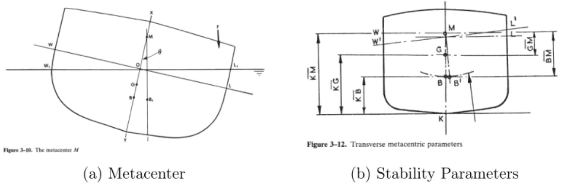
∙ M - The metacenter is used as a measure of a ship’s initial stability. As a ship rolls a small angle from its initial level position, the center of buoyancy will shift slightly as different parts of the hull go into or out of the water. If lines were to be drawn vertically from the original and disturbed centers of buoyancy, they would intersect at the metacenter. This is illustrated in Figure 1-4. The height

(a) Metacenter (b) Stability Parameters

Figure 1-4: Illustrations of the definition of a ship’s metacenter, and terms associated with determining initial stability. From Introduction to Naval Architecture[10]

of M above the keel is referred to as 𝐾𝑀 . The vertical distance from G to M, 𝐺𝑀 , is the most common measure of stability. A ship will be initially stable if it has a positive 𝐺𝑀 .

∙ LCF - The Longitudinal Center of Flotation of a ship is the point about which a ship will trim, or pivot forward and aft. It is located at the centroid of the waterplane (the plane where the hull intersects the water).

1.3

Project Overview

The following chapters describe the process and methods used for designing and analysing a modular ship model and ASV. Chapter 2 covers the design and construc-tion challenges of the hull and its control electronics, as well as the experiment setup for tow tank testing. Chapter 3 discusses the process of collecting and analysing data to model the performance of various iterations of the hullform. Finally, Chapter 4 discusses the potential for future work and outlines how the project may be used for future research and education.

Chapter 2

Design and Construction

The basic design needed for this thesis was for a modular monohull. A catamaran was then made from two elongated monohulls connected by two transverse brace bars. The baseline hull was specifically created to be adaptable over common ranges of form coefficients, including length, length-to-beam-ratio, draft, and prismatic coefficient.

(a) Assembled Monohull (b) Assembled Catamaran

Figure 2-1: Completed Baseline Hulls

2.1

Monohull Design

The design philosophy stipulated designing a low-cost vessel made up of additively manufactured segments which could easily be adapted to different desired payloads or functions. To achieve this goal, the main design point was to define the interfaces

between modules by determining the geometry of the parallel midbody. From there, a baseline hull was designed by defining a properly interfacing bow and stern. The final baseline monohull design is shown in Figures 2-1 and 2-2, consisting of four modules: the baseline bow, parallel midbody, baseline propulsion, and baseline stern. The process to develop the design is expounded on in the following sections.

(a) Isometric View

(b) Profile View

Figure 2-2: Baseline Monohull

2.1.1

Principal Dimensions

To facilitate construction, the design was made such that any segment could be built on any of the most popular fused deposition modeling (FDM) printers available, including Creality’s Ender 3 (build volume of 220x220x250mm) and Prusa’s i3 (build volume of 250x250x210mm) [18]. See Section 2.3 for a more thorough discussion of Additive Manufacturing. To maximize stability, the beam (B) was maximized at 200mm. Common beam-to-draft ratios range from 1.8 to 4 [10], so the lower was used to constrain the depth (D) to 120mm. Designed draft (T) was set at 60mm to be on the higher side of the beam-to-draft range and to provide a sufficient freeboard to avoid water ingress.

Length can be varied continuously and indefinitely, with the shortest possible configuration being a bow and stern connected together. This allows the design to accommodate varying payloads and missions, or to model a diverse group of ships, provided they maintain the same midships section.

2.1.2

Coefficients of Form and Parallel Midbody

Length to Beam Ratio

The length to beam ratio of most vessels varies from around 3 to 12 [10]. The length to beam ratio may be increased by adding more segments; therefore, the baseline hull was designed with an initial length-to-beam ratio of 3.

Midships Section Coefficient, Cm

𝐶𝑚 = 𝐴𝑚/𝐵𝑇

The Beam and Depth dimensional constraints define the maximum possible cross-sectional area of the vessel. This, coupled with a desired midships section coefficient Cm, defines the geometry of the parallel midbody. A Cmof 0.83 was chosen based on a

value from Gilmer and Johnson that is typical for faster and more maneuverable ships [10]. This yielded a desired midships sectional area, Am, of 9900 mm2. Discussion with

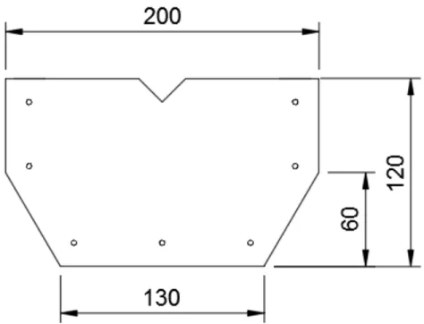
users of small unmanned vessels indicated a flat bottomed hull would be advantageous for storage and for shallow-water operations. Since a boxy, barge-like hull would result in excessive wave interaction, this narrowed the form of the midships section to a simple trapezoid, as show below in Figure 2-3. A flat-bottomed hull with a rounder profile would likely be more hydrodynamically efficient with less flow separation and vicious-eddy roll damping [10]. Designing such a hull, as well as hullforms with varying bilge keels, is a topic for future study. The same design process presented could be used for any desired midships section.

Prismatic Coefficient, Cp

𝐶𝑝 = ∇/𝐿𝐴𝑥

Due to the variable length of the design, a fixed prismatic coefficient cannot be defined. With a fixed maximum sectional area, 𝐴𝑥, the prismatic coefficient becomes a function

of length, 𝐿, and the displaced volume of the hull, ∇. If the design waterline, DWL, is kept constant, then ∇ will also increase linearly with length with the result being

Figure 2-3: Cross-section of Parallel Midbody (dimensions in millimeters). The seven holes around the perimeter are for M3 size bolts to connect modules together. The V-shaped notch in the top allows routing wires between modules while still securing the vessel with a lid.

𝐶𝑝 increasing with length and approaching 1.0 in the limit.

Block Coefficient, Cb

𝐶𝑏 = ∇/𝐿𝐵𝑇

𝐶𝑏 = 𝐶𝑝× 𝐶𝑚

Due to the above relationship between 𝐶𝑝 and 𝐶𝑏, the block coefficient will behave

the same as the prismatic coefficient, approaching the midships section coefficient in the limit.

Parallel Midbody (PMB) Module

Figure 2-3 was used to develop a baseline parallel midbody module. This module con-nected the bow and stern and provided volume for payload and buoyancy. Variations on the baseline PMB Module were made, including one with an integrated connection

point for model testing, and another with support structure to house a 12 volt lead acid battery for use in a self-propelled vessel.

2.1.3

Baseline Bow

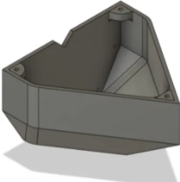
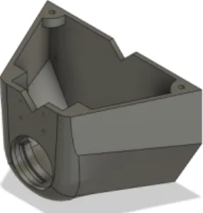
Figure 2-4: CAD rendering of hard-edged, baseline bow design

The baseline version of the bow was designed to have simplified geometry to support the design’s use in an educational environment. Its geometry makes it simple to calculate the model’s displacement exactly and to compare it with other methods, such as Simpson’s rule. The design mimics an ax-bow design by pointing the bow above the DWL. This style of bow has been shown to reduce resistance created from incident waves diffracting from the bow [14]. Smaller vessels, including ASVs of this model’s size, can be easily buffeted by small surface waves, even in protected waters; therefore, decreasing added resistance due to wave action was desirable.

2.1.4

Baseline Propulsion

(a) With Motor (b) Without Motor

Figure 2-5: Propulsion Module

One of the purposes of this thesis was to provide a platform capable of comparing various propellers and propulsion methods such as waterjets. As such, propulsion is contained within a single module with the expectation for future work to include creating different modules for comparison. For a baseline, the simplest possible stern was desired: a square stern. This will certainly introduce undesirable vortex shedding at the stern, not to mention poor inflow to the propeller, but that will be addressed and studied by follow-on designs. As for propulsion itself, inspiration was drawn from the maker community of Remotely Operated Vehicles (ROVs). A standard practice is to modify small sealed bilge pump cartridges due to their availability, cost, inherent water resistance, and power [22][15]. Additionally, there are many open-source designs for thrusters based on these bilge pump cartridges, providing ample ground for future investigations. For this project, a twist-lock interface was designed to mimic that of the pumps these cartridges are typically installed in. This twist-lock aids in sealing the propulsion module from the water. Additional fairing material was added around the twist-lock to add strength and ease the transition from the flat stern to the outboard portion of the motor housing.

Unfortunately, the diameter of these cartridges causes the propeller shaft to have only 11.5mm submergence. The International Association of Classification Societies recommends a propeller immersion of at least 25% of the propeller diameter [12].

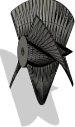
This in turn limits propeller size to 46 mm in diameter. Accordingly, a base propeller was designed with a diameter of 45 mm. The base propeller is a four-bladed helical design which is pressure-fit over a D-shaped flat on the propulsion motor shaft.

Figure 2-6: CAD rendering of Propeller

2.1.5

Baseline Stern/Steering

(a) Top View (b) Bottom View

Figure 2-7: Stern/Steering Module

In order to provide for steering, a stern sub-assembly was designed to extend over the top of the propulsion motor and propeller and serve as a mounting point for a rudder and steering servo. A waterproof servomotor mounts into the module and connects via a flexing tie-rod to a rudder linkage, which in turn connects to the rudder post. At the design displacement, most of this module is at or above the design waterline (DWL), so as not to contribute to the 𝐿𝑊 𝐿 and increase wetted surface area and frictional

resistance. The rising angle of the stern was made steep enough to create a clear path for the horizontal propeller wash. The length of the module permits sufficient clearance between the rudder and the propeller and also redirects propulsive energy that would otherwise be wasted in creating a rooster tail.

Rudder

The rudder itself was designed such that the rudder and rudder post could be printed together as a single piece, eliminating the need for a separate metal rudder post and simplifying construction. This did, however, introduce a minimum diameter for a sufficiently strong printed rudder post, so the baseline rudder was based on a NACA 0018 foil [2].

2.1.6

Rounded Bow

(a) Isometric View (b) Profile View

Figure 2-8: Rounded Bow

The rounded version of the bow retains the same overall geometry of the baseline bow, but uses a more conventional bluff-body shape seen in large cargo carriers which travel at low Froude numbers (Fn). This is generally a desirable geometry due to its lower

resistance in calm waters [7]. Its fuller shape also takes greater advantage of the available volume, increasing the resulting model’s Cb and Tons Per Inch Immersion

(TPI). It does, however, result in a greater frictional resistance due to its greater wetted surface area.

2.1.7

Rounded Propulsion

Figure 2-9: Rounded Propulsion Module

The rounded propulsion module is an attempt to fair the hull and streamline the flow into the propeller. Its aft face deviates from the standard parallel midbody used in the baseline variant and includes mounting holes and access specifically for the streamlined stern module below.

2.1.8

Rounded Stern/Steering

(a) Stern/Steering Module (b) Combined Propulsion Module

Figure 2-10: Rounded Stern/Steering Module

The rounded stern module terminates the aft end of the ship in a teardrop shape, pro-viding only enough structure to include a servo for steering. Unlike the baseline stern, the rounded stern is designed to use a waterproof servo mounted on the underside of the vessel with a direct connection to a rudder instead of using a linkage.

2.1.9

Stability Experiment Lid

Figure 2-11: Lid designed for stability experiments

A lid was designed to attach to the baseline vessel’s parallel midbody section. Posts were spaced transversely in 25mm increments with recesses to hold cylindrical weights. This was used to conduct an inclining experiment in order to determine the vessels vertical center of gravity (KG). Additionally, the lid has bolt holes for connecting a length of 8020 extruded aluminum which extends vertically above the ship and can be fitted with a weight on a sliding collar. This allows for shifting the vertical center of gravity of the ship in order to conduct experiments on roll period and stability, as discussed in Section 4.1.1.

2.1.10

Remote Control and Autonomy Electronics

In order to be used as a free-running model, a parallel midbody module was designed to house a 12 volt lead acid battery and other control and sensing electronics. For sensing, the design includes a combined Compass / Inertial Measurement Unit (IMU) and a Global Positioning System (GPS) receiver and antenna. These are controlled via an Arduino micro-controller and data can feed over USB serial to a Raspberry Pi single-board computer for data logging, and/or control. Control actuation is accom-plished by the Arduino via a brushed-motor Electronic Speed Controller (ESC) for the propulsion motor, and a servomotor for rudder control. A 12 Volt bus bar pro-vides power via fork and spade solderless connectors to the Arduino’s internal voltage regulator, the propulsion motor’s ESC, a micro-USB power supply for the Raspberry Pi, and a 12-to-5 volt voltage regulator which powers a separate 5 volt bus. The 5 volt bus similarly powers the rudder servomotor, a remote control receiver, the GPS, and the IMU. A common grounding bus is used for all components to prevent ground loop interference. A pair of 5v switching relays is used to toggle between remote control and on-board control. A diagram of the electrical system can been seen in Figure 2-13.

1 2 V S e a le d L e a d A c id B a tte ry R C C h a n n e ls : 1 - P o w e r/G ro u n d 2 -2 -3 -4 - A u to n o m y S w it c h (R e la y C o n tro l) 5 - R u d d e r 6 - T h ro tt le 1 2 v: -1 2 V t o 5 V U B E C ( 5 V B u s ) - A rd u in o ( V in ) -1 2 V t o 5 V U S B ( R a s P i) -P ro p u ls io n M o to r ( via E S C ) 5 V : -R u d d e r S e rv o P o w e r -R C R e c e iv e r -G P S /IM U B re a d b o a rd N o m in a l w ir in g s h o w n . D o e s n o t s h o w I2 C /S e ria l c o n n e c tio n s t o A rd u in o . A c tu a l G P S /IM U m o d u le s d iffe r.

In many experiments it is desirable to have the free-running model under au-tonomous control. For example, M. Míguez González, et al. designed a free run-ning ship model to conduct experiments in parametric rolling and other seakeeping experiments where connection to a carriage is excessively restrictive [11]. Limited course-following, station keeping, or preprogrammed routines can be implemented on the Arduino alone, but more complex automation is best done on a dedicated computer. In this design, the Raspberry Pi single board computer can communicate via serial with the Arduino. MOOS-IVP software running on the Raspberry Pi can receive sensor data from the Arduino, compute a desired heading and speed based on the loaded autonomy package, and pass those orders on to the Arduino for execution via the propulsion ESC and rudder servo [19]. The rudder and motor control signals are routed though a pair of switchable relays which can be toggled via an auxiliary channel on the remote control. This allows an operator to take remote control in the event of an autonomy failure.

Remote control, when selected via the remote control’s auxiliary channel, is typ-ically accomplished by two channels controlling the servomotor and the motor ESC. When configured as a catamaran, each channel is instead used for a separate propul-sion ESC, allowing for differential steering.

2.1.11

Baseline Monohull

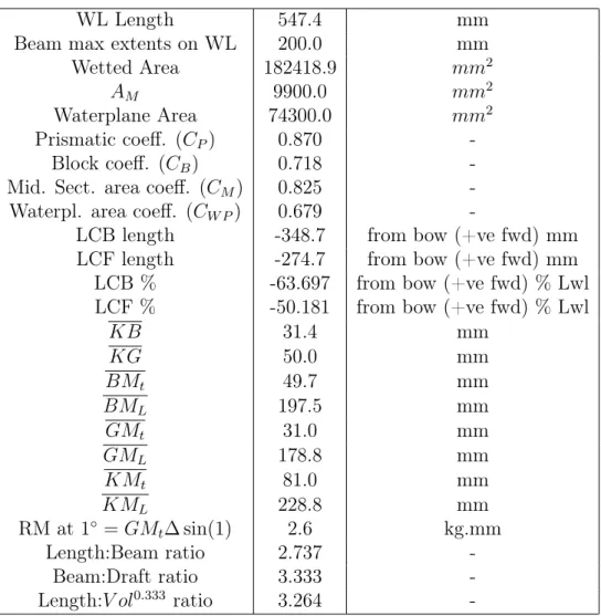
Combining the baseline bow, parallel midbody, propulsion, and stern modules created what is further referred to as the Baseline Monohull. While a smaller version could be made by removing the parallel midbody module, the baseline version is the smallest variant that includes all the modules. A version was made with the parallel midbody modified to hold a battery, and a version was made with the parallel midbody modified to connect with the towing carriage connector described in Section 2.4. An image of the baseline monohull is found in Figure 2-2. The baseline monohull was recreated and analysed in the MAXSURF software suite with the resulting hydrostatic data presented in Table 2.1.

WL Length 547.4 mm Beam max extents on WL 200.0 mm

Wetted Area 182418.9 𝑚𝑚2

𝐴𝑀 9900.0 𝑚𝑚2

Waterplane Area 74300.0 𝑚𝑚2

Prismatic coeff. (𝐶𝑃) 0.870

-Block coeff. (𝐶𝐵) 0.718

-Mid. Sect. area coeff. (𝐶𝑀) 0.825

-Waterpl. area coeff. (𝐶𝑊 𝑃) 0.679

-LCB length -348.7 from bow (+ve fwd) mm LCF length -274.7 from bow (+ve fwd) mm LCB % -63.697 from bow (+ve fwd) % Lwl LCF % -50.181 from bow (+ve fwd) % Lwl

𝐾𝐵 31.4 mm 𝐾𝐺 50.0 mm 𝐵𝑀𝑡 49.7 mm 𝐵𝑀𝐿 197.5 mm 𝐺𝑀𝑡 31.0 mm 𝐺𝑀𝐿 178.8 mm 𝐾𝑀𝑡 81.0 mm 𝐾𝑀𝐿 228.8 mm RM at 1∘ = 𝐺𝑀𝑡∆ sin(1) 2.6 kg.mm Length:Beam ratio 2.737 -Beam:Draft ratio 3.333 -Length:𝑉 𝑜𝑙0.333 ratio 3.264

-Table 2.1: Principal Characteristics of the Baseline Hull from Maxsurf

2.2

Catamaran Design

Figure 2-14: Free-running Catamaran

A catamaran was designed by removing the steering module and adding another parallel midbody section to the baseline monohull. Steering was accomplished via differential powering, eliminating the need for rudders and their associated modules.

Two of these hulls were built and connected to one another via 80/20 extruded alu-minum. The existing bolt holes used to secure the vessel lids were reused with longer bolts to mount the 80/20 angle brackets on top of the bow and propulsion module lids. While only the one configuration shown in Figure 2-14 was created, the intent is to be able to vary demihull spacing. This enables future researchers to study demihull wave interaction, effect of demihull spacing on maneuvering coefficients and turning radius, or simply to permit mounting additional hardware between or outboard of the two hulls. Due to its improved stability under virtually all conditions, the catamaran variant is expected to be the most useful for open water experiments and for use as an ASV. Its greater available displacement allows for more involved payloads, includ-ing extra batteries for endurance and sensors for mission needs. An adaptor plate was designed and printed to allow connecting the catamaran to the towing carriage. Contrary to ITTC recommendations, the connection is above the line of thrust from the propellers, so compensation will be needed for the additional moment induced about the transverse axis. [9]

2.3

Additive Manufacturing

This project focuses on the use of additive manufacturing for actualizing new hull designs. The most prevalent form of additive manufacturing uses a technology called Fused Deposition Modeling (FDM). As the name implies, FDM printers heat a ther-moplastic polymer filament to its melting point and deposits layers of melted filament on top of one another, fusing them together and building up the desired shape.

2.3.1

Materials

Different materials can be used with FDM printers, with the most common being PLA, ABS, and PET-G. All three have their strengths and weaknesses and all three were used or tried over the course of this project.

∙ ABS - Acrylonitrile Butadiene Styrene is one of the first materials used with FDM printers. It is strong and has a high melting point, making it stable

under most use cases. A particular advantage of ABS printing is its solubility in acetone. There are techniques that take advantage of this attribute in order to smooth out the ridges between sequential layers that are inheirent in all FDM printed parts. This can remove stress concentration areas and create a seamless, waterproof finish. The major disadvantage to printing with ABS is that it is difficult to print large objects without the part cooling below its high glass transition temperature of 105 C before it is finished. This causes internal stresses which cause the part to contract and warp, loosing its shape. This can be mitigated by enclosing and heating the printer, but such printers or modifications are not standard and were not available for this project. Only one module was made with ABS, and while it was successfully waterproofed with acetone, it had lost its dimensional accuracy due to warping.

∙ PLA - Polylactic Acid has become one of the most prevalent fillaments on the market due to its ease of use. Its lower printing temperature and glass transition temperature make it much easier to work with and maintain its shape. It is more brittle and weaker than ABS and is not usually used for heavily loaded parts without reinforcement. This material was used extensively in this project. ∙ PET-G Polyethyline Terephthalate Glycol is a more recent entry to the FDM filament scene. It has the low glass transition temperature of PLA and the strength of ABS. It holds its shape well, but with a higher melting point than PLA and ABS, it can sometimes be difficult to maintain a consistent quality with larger parts. This material was also used extensively for this project.

2.3.2

Waterproofing

While it is possible to get waterproof results using FDM printing, it is by no means commonplace. Overextrusion, large nozzel sizes and layer heights, thicker walls, and experimental continuous extrusion methods were met with mixed success. Post-processing of printed modules can be time consuming, so experimenting with different techniques to achieve an off-the-printer waterproof module was worthwhile, although

ultimately fruitless. In the end, an epoxy coating was found to be the most effective, but other researchers have found success with spray-on urethane coatings.

Without Post-Processing

Test cubes were printed in PET-G filament using nozzles varying from 0.4mm to 0.8mm. The thickness of shell layers in the walls was varied from 2 nozzle diameters (one inner and one outer layer) to 8 (creating a solid cube with the smallest nozzle). Water was dyed blue for visibility and two leak tests were performed. First, empty cubes were floated in a basin of water for one hour. This tested the water permeability through the outer wall’s layers. The cubes were dried and any leakage allowed to drain. For the second test, the cubes were placed in an empty basin and filled with dyed water. This tested water permeability through the inner wall.

(a) Float Test (b) Fill Test

(c) Interstitial Voids

Figure 2-15: Waterproofing Tests - 0.6mm Nozzle

and with at least two inner and two outer walls was able to prevent any water ingress to the cube’s interstitial voids. Unfortunately, water did leak through at the interface between the floor of the cube and the wall of the cube, even though the floor was printed with the same number of layers. This can be seen in Figures 15c and 2-15a. While it is possible that increasing the shell thickness or adjusting more settings may have yielded a perfectly waterproof print, it became evident that the time spent adjusting printer settings (which may differ between printer types) would quickly outpace the time spent in applying a coating system. Additionally, the added layers and increased infill of the print would increase the vessel’s weight and cost more than a coating system would.

Aerosol Rubber Coating

Inspired by claims that a screen door could be rendered waterproof by the application of an aerosol rubber spray called Flex Seal, such a product was used to attempt to waterproof a printed module. Flex Seal creates a rough surface finish which would be detrimental to model testing, so Plasti-Dip was used instead. Unfortunately, the aerosol spray seemed to create air bubbles in each coat which made each layer slightly porous, regardless of the thickness of the coat. Even after 6 coats, a ballasted module that was left waterborne sank after 12 hours. The vessel shown in Figure 2-12 is coated on the outside with Plasti-Dip.

Paintable Rubber Coating

To avoid the aerosol-induced pores from the spray on coating, a paintable product simply called Liquid Rubber was used. It created a rougher surface finish than the Plasti-Dip, but did produce a waterproof result in a single, thicker coat. The coating remained tacky even when cured, so it would require further treatment. This was deemed suitable when using this thesis’ design for a remote control or autonomous vessel, but would not be an adequate surface finish for model testing.

Epoxy Resin

The most labor-intensive finish yielded the best results. Traditionally, ship models are made from cut foam, coated in fiberglass, and saturated with epoxy. Two types of epoxy resin were tested with virtually identical results. XTC-3D is a thin epoxy specifically engineered for coating 3D printed parts. Its low viscosity allows it to more easily penetrate a 3D print’s pores. Total Boat Epoxy with a fast curing hardener was also used. It is a thicker marine epoxy used in boat repair and had adequate penetration to seal a printed module. Epoxy coating required a more extensive surface preparation and time between coats. It also required follow-on sanding to smooth the resulting coat since the 28th ITTC Resistance Committee [8] showed that unfinished 3D printed models do not meet requirements for surface smoothness. The models need to be sanded with at least 300-400 grit sandpaper to meet these requirements. Epoxy coated models used for model testing can bee seen in Chapter 3.

2.4

Towing Carriage

The MIT Tow Tank was originally designed for model testing ships, but in recent years had been converted for research in biomimetics, vortex-induced-vibrations (VIV), and flow visualization. To conduct a series of ship model tests, the carriage attachment was rebuilt and instrumented. As shown in Figure 2-16, the model attachment from an older model of a DDG51 hull was reused to make a standard mounting point. This included a hinge allowing the model to pitch freely, as recommended by the ITTC [9]. An adaptor plate/box connected the hinge to the force sensor, an AMTI MC3-SSUDW [3]. The MC3-SSUDW is a six-axis strain-gauge force sensor rated for submerged freshwater use. It is factory calibrated and when used with its accompanying data acquisition software, calibration and data conversion are transparent to the user. An optic rotation mount was modified and installed atop the force sensor to enable adjusting the drift angle of the model. This permitted conducting captive model maneuverability tests per section 7.5-02-06-02 of the ITTC Recommended Procedures and Guidelines Manual [9]. This mount in turn attached to the base plate of a pair

Figure 2-16: Resistance Experiment Rig

of linear bearings with ball bushings, serving as heave posts. These allowed the ship to freely move in the heave direction, as per ITTC recommended procedures for resistance modeling [9]. Finally, the heave posts were mounted to a frame made of extruded aluminum which connected to the towing carriage and the tow tank was ready for experimenting.

Chapter 3

Captive Model Testing

All hulls designed for this project are referred to as models in this chapter. Hulls intended to be used as autonomous or remote controlled vehicles are treated as 1:1 scale models. Model testing was performed on a ship model with known characteristics in order to validate the equipment setup and data analysis process. Then, the baseline hull made in Chapter 2 was tested with two different coating systems. Next, the utility and flexibility of the design was demonstrated by performing a study on two variations of the baseline hull. The data was then used to guide the design of a large unmanned vessel. A larger model of the final design was created and tested, with results compared to empirical methods of predicting resistance and to the preliminary models.

3.1

Resistance Testing Implementation

Captive model testing was performed in the MIT Towing Tank, a 108-foot long, 8-foot 7-inch wide basin equipped with a towing carriage, wave maker, and wave absorption beach. The size of the tank is ideal for models around 4 to 6 feet long [1]. Smaller models can be used, but model testing results are always more accurate with larger models and their respectively smaller scale factors and higher Reynold’s numbers. The MIT tank is equipped with a 600 lbs carriage which can be run at speed up to 1.6 m/s. Higher speeds up to 2.5 m/s can be achieved, but with additional acceleration

induced jerk and shorter spans where clean test data is acquired at the requested speed [23].

Figure 3-1: Flow regimes along a hull from Introduction to Naval Architecture[10]

The biggest downside to a smaller towing tank and correspondingly sized models is a low Reynolds number, typically associated with the laminar or transitional flow regimes. For example, the waterline length of the Baseline Monohull tested in this thesis is only 0.6 meters. This put it entirely in the laminar flow regime at speeds less than one knot (0.514 m/s), and in the transition regime all the way up to an unattainable 17 knots (8.745 m/s). This becomes a problem if the hull being tested in the tank is intended to model a larger ship, since the model will not be in the same flow regime as the full scale vessel, which is almost always in a turbulent regime. Figure 3-1 from Gilmer and Johnson [10] shows the development of turbulent flow along a ship’s hull. This introduces significant error in the results due to the greater skin friction associated with turbulent flow. A standard practice is to "trip" the flow

of water across the model by increasing surface roughness near the bow. This causes the flow to become prematurely turbulent and raise the skin friction to a closer scaled approximation of what it would be at full scale. The models used in the following experiments did not use any such turbulence trippers since they were intended to be used as ASVs after model testing was complete. If turbulence trippers are desired, studs could easily be added to a bow module and printed in place at the anticipated transition point. Procedure 7.5-01-01-01 of the ITTC Recommended Procedures and Guidelines [9] governs model manufacture and recommends turbulence trippers be placed 5% Lpp aft of the forward perpendicular.

ITTC Procedure 7.5-02-02-01 expounds on the best practices for the conditions and setup for resistance tests [9]. Control surfaces such as rudders are not typically installed for resistance tests, unless they form a continuation of a skeg. This was not the case for the series of experiments described below, so rudders were not installed. The propulsion motor was installed on the Baseline Monohulls since it forms an integral part of the stern, but in most cases a propeller was not attached to the hub to avoid the additional drag created by a stationary or trailing propeller. The towing connection was placed as close to the line of thrust from the propeller shaft as was practicable, and placed at the approximate longitudinal center of buoyancy to avoid inducing an artificial trim. The baseline hulls were ballasted to achieve the same draft and displacement as the free-running hull when loaded with its control electronics.

3.2

Data Collection

As described in Section 2.4, an AMTI MC3-SSUDW six-axis force sensor was used to measure the horizontal towing force needed to tow the hull through the water at the ordered speed of the towing carriage. The force sensor, in turn, was connected to an AMTI GEN5 signal processor which provided excitation voltage to the wheat-stone bridge strain gauge elements and also provided signal amplification and serial conversion. The GEN5 was connected via USB to a laptop on the towing carriage which was running AMTI’s NetForce software for data acquisition and storage. The

NetForce software conveniently applies calibration data to the raw voltage signal, al-lowing the user to work with force data in either english or metric units. This data was transferred remotely to another computer for data analysis. While unused for these experiments, orientation and acceleration data from an on-hull inertial measurement unit could be measured via the towing carriage’s BNC connections.

Test parameters were recorded for future reference, including: the date data was taken, water depth in the tank, presence/absence of turbulence tripers, bare hull weight/displacement, towing rig weight supported by the model, ballast weight, draft forward, draft aft, LWL, scale factor, and planned towing speeds. Each data run was set to last for one minute to fully capture data at the slowest towing speed (typically around 0.1 m/s). Data runs at higher speeds were ended after the towing carriage came to a stop and all unused space in the data buffer was assigned a zero value. Data was taken with a sampling frequency of 40 Hz to account for Nyquist requirements. A typical data run, as shown in Figure 3-2, began with the model at rest with no force being applied. The carriage was then started, resulting in a rapid acceleration up to the commanded tow speed and a corresponding spike in tow force. Once the ordered speed was achieved and the carriage was moving at a steady rate, the force dropped down to the steady-state towing force. Some force oscillations occurred due to coupling of the stiffness of the towing rig and the towed body, but they were later removed by filtering and time averaging the steady-state data. Toward the end of the data run, the carriage decelerated and stopped, resulting in another force spike before speed and force measurements returned to zero.

3.3

Data Analysis

Data analysis was performed with the MATLAB script found in Appendix A. This section walks through the stages in the code and some of the theory behind it.

Based on Froude’s original hypothesis for model testing and modern ITTC guid-ance, resistance data is converted from model scale to full scale by extracting the model’s wave-making resistance from its total resistance. This is done by subtracting

(a) Low Speed (b) High Speed

Figure 3-2: Unfiltered data collected at low and high speeds, showing the initial acceleration, steady speed, and deceleration stages.

the resistance due to frictional and other residual effects from the total measured model resistance. This resulting wave-making resistance can then be scaled up to the full ship size and speeds based on the non-dimensional Froude number, 𝐹𝑛 = √𝑉_𝑔𝐿.

The full scale ship’s frictional resistance is then added based on analytical methods to arrive at a final total resistance for the ship.

Certain test parameters must be hard-coded in the code’s preamble, such as tank water density, scale factor (𝜆), model length, and model wetted surface area. Testing velocities must be entered in a vector which is also polled by the script to extract data from the data run files. Test speeds are chosen such that the model speeds (𝑉𝑀)

match the Froude number for the full scale ship speeds (𝑉𝑆) of interest.

𝑉𝑀 √ 𝑔𝐿𝑀 = 𝐹𝑛= 𝑉𝑆 √ 𝑔𝐿𝑆 𝜆 = 𝐿𝑆 𝐿𝑀 𝑉𝑀 = 𝑉𝑠 √ 𝜆

3.3.1

Data Selection and Filtering

The first section of the script iterates through the vector of speeds, finds and extracts the x-axis force data from its corresponding data log, and applies a low-pass filter to

eliminate the noise from the data. The force sensor is oriented with the bow in the +𝑥 direction, so all towing forces are initially recorded as negative values but the script changes the sign convention so they are positive. The script then pulls up the filtered data on a graph one at a time and prompts the user to tare the data by selecting a range where the model was stationary. The dataset is then replotted with the average of the stationary region subtracted from the set. The user is then prompted to select the region of the data where the carriage was at a constant speed, eliminating the force spikes on both ends caused by carriage acceleration. The selected data is then time-averaged to yield a steady-state tow force.

Figure 3-3: Screenshot of graphical data selection

3.3.2

Model’s Total Resistance Coefficient (𝐶

) and

Fric-tional Resistance Coefficient(𝐶

)

Equation 3.1 is applied to the model’s average total towing resistance, 𝑅𝑇 𝑀, yielding

the model’s non-dimensional total resistance coefficient, 𝐶𝑇 𝑀 for each speed.

𝐶𝑇 𝑀 = 𝑅𝑇 𝑀 1 2 * 𝜌𝑀𝑆𝑀𝑉 2 𝑀 (3.1)

This data is plotted against tested speeds, with the non-dimensional total resistance coefficient also being plotted against the non-dimensional Froude Number.

The model’s frictional resistance coefficient, 𝐶𝐹 𝑀, is then found from the ITTC-57

model-ship correlation line:

𝐶𝐹 =

0.075

log₁₀(𝑅𝑒 − 2)2 (3.2)

3.3.3

Prohaska’s Form Factor

The ITTC-57 friction line is based on experiments with flat plates. Additional viscous effects due to the shape of the hull exist, even at slow speeds where wave-making drag is not significant [9][10]. Thus, a form factor, 𝑘, is calculated using Prohaska’s method and then applied to the frictional resistance coefficient to prevent attributing this extra resistance to wave-making and improperly scaling it.

𝐶𝑇 𝑀 = (1 + 𝑘)𝐶𝐹 𝑀 + 𝐶𝑊 (3.3)

Prohaska’s method assumes that at low speeds, a ship’s wave-making resistance is a function of the Froude number to the fourth power. Based on this assumption, the ratio of the total resistance coefficient and the frictional resistance coefficient (𝐶𝑇 𝑀

𝐶𝐹 𝑀) will equate to 1 + 𝑘 when the speed approaches zero. In the code, the user

must input which speeds should be used to calculate this form factor, with typical speeds corresponding to Froude numbers between 0.1 and 0.2. The code then plots the relationship and derives a form factor.

Other methods may also be used to empirically determine form factor, such as the Watanabe formula [16]:

𝑘 = −0.095 + 25.6 * 𝐶𝐵 (_𝐵𝐿)2

*√︁𝐵 𝑇

(3.4)

If this is the case, a value for form factor can be hard-coded to overwrite the Prohaska value.

Figure 3-4: MATLAB Figure showing derivation of Prohaska’s Form Factor

3.3.4

Extrapolation to Full Scale

Once form factor has been determined, it can be applied to extract the non-dimensional wave-making resistance coefficient, 𝐶𝑊, via Equation 3.3. 𝐶𝑊 is applicable for both

the model and full scale ship since the experiment was performed at speeds scaled by Froude number. The frictional resistance coefficient of the full-scale ship (𝐶𝐹 𝑆)is

calculated using Equation 3.2 (using the full scale Reynolds Number). Additional factors such as air resistance (𝐶𝐴𝐴𝑆), roughness (∆𝐶𝐹), and a facility-specific

corre-lation allowance (𝐶𝐴) can be factored in for additional precision to reach a final total

𝐶𝑇 𝑆 = (1 + 𝑘)𝐶𝐹 𝑆+ 𝐶𝑊 + ∆𝐶𝐹 + 𝐶𝐴+ 𝐶𝐴𝐴𝑆 𝑅𝑇 𝑆 = 1 2𝜌𝑆𝑉 2 𝑆𝑆𝑆𝐶𝑇 𝑆

𝜌𝑆 is density of the ship’s fluid medium (typically saltwater) and 𝑆𝑆 is the wetted

surface area of the full scale ship.

In most cases, the desire to predict the resistance of a vessel stems from a need to determine power requirements in order to size an appropriate propulsion plant. Effective power is calculated by multiplying the towing resistance and the speed.

3.4

Methodology and Performance Validation

In order to validate the methodology presented above, the first model tested and evaluated was a 1/100th scale DDG51 hull with known characteristics and power requirements. The model was ballasted to the design waterline and scaled test speeds were calculated for speeds from 1 to 35 knots in 1 knot increments. The model was run and data evaluated with the results presented in Figure 3-5. Of particular note is Figure 3-5f, where the model testing results match known powering data almost perfectly, thus validating the approach.

3.5

Baseline Hull Testing

Since the baseline hull was not designed to model a specific larger vessel, testing on the baseline was performed with a scale factor of 1 to evaluate the performance characteristics of the hull for use as an Autonomous Surface Vehicle. The resulting resistance data was then used for comparison of hull coatings and in future work can be used to determine estimated endurance for a given motor and battery. Future studies can also evaluate the effect of additional appendages, modules, bow and stern

(a) Model Resistance vs Speed (b) Model Total Resistance Coefficient vs Froude Number

(c) Results of Prohaska’s Experiment to de-termine form factor

(d) Resistance Coefficient separated into frictional and wavemaking components

(e) Predicted Resistance at full scale (f) Effective Power for full scale ship,

compared with given data from ASSET

shapes, etc. on the baseline hull. Prohaska’s method produced poor results for this hull, likely due to observed flow separation at the knuckle of the bow and at the hard edge of the stern. The Watanabe formula in Equation 3.4 was used and yielded a form factor of 1.4. Additional correction terms ∆𝐶𝐹, 𝐶𝐴, and 𝐶𝐴𝐴𝑆 were not applicable

and went unused.

3.5.1

Baseline - Rubber Coated

Figure 3-6: Resistance Data for a rubber coated baseline hull

The first hull tested was a baseline hull with a spray-on rubber coating. The rubber coating was not particularly smooth, but no attempt was made to quantify its surface roughness. This hull can be seen attached to the towing rig in Figure 2-1a. When self-propelled, the hull was observed to reach speeds of 0.5 m/s. Test speeds were chosen to encompass this observed speed, ranging from 0 to 0.75 m/s in 0.125 m/s increments. Resulting resistance data is presented in Figure 3-6.

3.5.2

Baseline - Epoxy Coated

Figure 3-7: Resistance Data for an epoxy coated baseline hull

The next hull tested was a baseline hull with an epoxy coating. The coating was wet sanded up to 1200 grit, resulting in an especially smooth hull. Resistance data is presented in Figure 3-7.

3.5.3

Baseline Conclusions

Figure 3-8: Comparison of hull resistance with rubber and epoxy coatings

There is little difference in the resistance between the two coating systems. Contrary to expectations, the smoother epoxy coated hull had a slightly higher resistance. This may be due to slight variations in displacement or be within the margin of error for this analysis. Regardless, the coating system does not appear to have a significant effect on the hull’s resistance at these speeds and this scale. If the hull is to be used as an ASV, the choice of hull coating can be relegated to personal preference and convenience.

3.6

Case Study - 16 meter USV

The following case study is presented to demonstrate the utility of this design and framework for conducting preliminary model testing in support of the design of a larger unmanned vessel.

3.6.1

Background

Unmanned vessels tend to have missions lasting for several hours and in some cases for several days. Recent developments in energy harvesting are extending endurance for small unmanned vessels up towards a year, such as with the Liquid Robotics’ Wave Glider or Saildrone’s Saildrone[20] [21]. These technologies do not scale up favorably, but there is still a desire to have a large unmanned platform capable of year-long missions.

A feasibility study was requested for a 16 meter vessel capable of a 1-2 year mission while carrying a payload packaged in a 20-foot shipping container. To meet this endurance requirement while relying primarily on solar power supplemented by hydrogen fuel cells, top speed was limited to 5 knots. There were concerns that this low speed regime may be too far out of the traditional design space that typical power prediction methods are optimized for. Since power consumption was paramount in the design of the vessel, model tests were conducted to validate empirical methods and to inform design choices regarding form.

3.6.2

Informing Early Design Choices

Theoretically, at slow speeds a vessel’s hull form could be designed from flat plates as opposed to traditional compound curves without significant impact to resistance. The advantage of a flat plate hull would be simplicity and economy of manufacture due to fewer plate bending operations. Conversely, other research indicated a stream-lined hull with a pointed bluff bow (also referred to as a LEADGE bow) would be significantly superior [6]. In order to determine which design philosophy best achieved the design goals for the vessel, two models were made at 1/20th scale and are shown in Figure 3-9. The first model was made by elongating this project’s baseline design with a plug module forward of the main parallel midbody section. The second was made using the rounded bow and rounded stern modules, again with a plug module installed forward of the parallel midbody module. This proved to be a problem, since the second model’s Longitudinal Center of Buoyancy was then located forward of the

towing attachment. This created an artificial trim effect and induced some longitu-dinal instability at higher speeds, so the test runs were limited to a scaled 5 knots. Placing the plug aft of the towing connection would have prevented this problem. Both models had the same beam, length, midships sectional area, and approximate wetted surface area once properly ballasted.

(a) Flat Plate 1/20th scale Model (b) Rounded 1/20th scale Model

Figure 3-9: 1/20th scale models used to inform early design choices

(a) Flat (b) Rounded

Figure 3-10: Power requirements for flat plate and rounded designs scaled to full size

Powering results are shown in Figure 3-10, which shows the rounded vessel re-quiring approximately 10kW at 5 knots compared to the flat plate vessel rere-quiring approximately 14kW at 5 knots. With power requirements for the flat-plate vessel ex-ceeding those of the rounded vessel by 20-40%, subsequent effort went into optimizing

a rounded hull form.

3.6.3

1/10th Scale Hull

A hullform was created in the MAXSURF software suite based on the results from a study of ideal hullforms for slow speed, wave efficient designs [6]. The body plan is similar to the KW-Supramax design and features a LEDGE-bow to maintain low resistance in short waves. To validate MAXSURF’s resistance predictions, a 1/10th scale model of the hull was created. This hull was also rapid prototyped using fused deposition modeling (FDM) and epoxy, but due to its scale it did not follow the modular methodology laid out in Chapter 2.

(a) Under construction (b) Attached to experiment rig

Figure 3-11: 1.6 meter long ship model

The model was towed at Froude-scaled speeds equivalent to 1-6 knots in half-knot intervals. Resistance data was collected and analysed. Prohaska’s experiment to determine form factor per the current ITTC Recommended Procedures was deemed inappropriate since the entire operating profile of the ship and model are at low

Froude numbers. Instead of using the modern form-factor method for extrapolating test data to full scale, Froude’s original method of separating resistance into frictional and residual resistance was used. With this method, the ITTC-57 friction line is used to estimate frictional resistance of both the model and the full scale ship. This estimated frictional resistance is subtracted from the model’s tested resistance, and the remaining resistance is attributed to wave-making and other effects which can be scaled by Froude number. This is equivalent to using a form factor of 0. Figure 3-12 shows the experimental results for these components of resistance.

Figure 3-12: Full Scale Resistance broken up into Frictional and Residual (Wavemak-ing) Resistance

3.6.4

Case Study Conclusions

Figure 3-13 plots the effective power estimate from the tank test results in blue alongside the theoretical values from various empirical methods. Holtrop’s updated

Figure 3-13: Comparison of Model Testing Power Prediction and Analytical Methods

method of predicting power was applied in a python script. The frictional and total power resulting from this Holtrop script are shown in yellow and red respectively. The power calculated by MAXSURF for the hullform is shown in purple. As seen, model testing results tracked well with the predicted power demands. Additionally, full scale results based on the small preliminary rounded hull were within 16% of the results from the larger, more accurate model. This validates its use as a first-pass gauge of a design’s viability. It is worth noting that both large and small models lacked turbulence trippers. Measured resistance would have increased due to the increased frictional resistance had turbulence trippers been installed.

3.7

Captive Model Testing Conclusions

This Chapter successfully validated the experimental setup and analysis, yielded ini-tial data on the baseline hull, and validated the utility of the project for conducting preliminary design of unmanned vessels. The stage is now set for future captive model tests. Chapter 4 provides a more detailed discussion of future work. In brief, additional studies should be performed to quantify the performance characteristics of

the catamaran design. Additionally, the rig was designed with the aim of performing experiments to determine a vessel’s maneuvering coefficients and in turn to design a control system for the models. Future work should consider these analyses as a priority as they will unlock the ability to perform free-running model testing.