The design, analysis, construction, and testing of a multifunctional composite satellite structure

OCf1.0WGY

EP0 7 2000

B.S., Aerospace Engineering (1995) The Pennsylvania State University, Pennsylvania

Submitted to the Department of Aeronautics and Astronautics in Partial Fulfillment of the Requirements for the Degree of

Master of Science in Aeronautics and Astronautics at the

Massachusetts Institute of Technology -May 2000

@2000 Massach~usetts Institute of Technology All rights reserved

Signature of Author ... 6.1...

Aeronautics and Astronautics May 19, 2000

... Hugh L. McManus

-incipal Research Engineer ,Thesis Supervisor -uepartment or Certified by ... 1-% 1 1 Accepted by ...

...

... ..

...

THE DESIGN, ANALYSIS, CONSTRUCTION, AND TESTING

OF A MUL TIFUNCTIONAL COMPOSITE SATELLITE

STRUCTURE

by

THE DESIGN, ANALYSIS, CONSTRUCTION, AND TESTING OF A

MULTIFUNCTIONAL COMPOSITE SATELLITE STRUCTURE

by

Christopher T. Dunn

Submitted to the Department of Aeronautics and Astronautics on May 19, 2000 in partial fulfillment of the requirements for the Degree of Master of Science in Aeronautics and

Astronautics

ABSTRACT

A small space based telescope is being designed by the Charles Stark Draper Laboratory, Inc. in conjunction with MIT. The design goal of this project is to use existing technology to gather ground data from low earth orbit at a minimal cost. A structure was constructed at MIT that allows the satellite to survive launch loads and maintains the optical stability of the satellite. The structure is a double hull design constructed of AS4/3501-6 graphite epoxy with a zero coefficient of thermal expansion lay-up to prevent defocusing of the optics due to thermal loading. The overall design goal at MIT is to construct a space worthy structure. This thesis includes the preliminary design of the inner structure that houses the optics for the telescope. Design of the outer structure, the connections between the inner and the outer structure and detailed design of the inner structure are not included in this work.

The analytical techniques used in this project included thermal analyses of structures in various earth orbits, determination of structural requirements from optical performance calculations, designing of near zero Coefficient of Thermal Expansion (CTE) laminates, consideration of manufacturing and material variations in design, strength analysis of composite laminates, and determination of vibration modes and associated frequencies of tubular structures with anisotropic sandwich construction.

Experimental work included the building of co-cured honeycomb panels, curved panels, and tubular sections to verify the structure as designed was manufacturable. These efforts culminated in the production of a space-worthy component.

Testing was preformed to verify the analysis and design. Testing included flatwise tension testing to verify integrity of the honeycomb bonding, tensile testing to verify stiffness calculations and experimentally determine the failure load for the desired lay-up, and testing to verify the CTE was within acceptable bounds to prevent the optics from defocusing.

Thesis Supervisor: Hugh L. McManus

FORWARD

This research was completed at the Technology Laboratory for Advanced Composites at the Massachusetts Institute of Technology. This work was supported by the Charles Stark Draper Laboratory, Inc. under IR&D contract DL-H-484763.

TABLE OF CONTENTS

2.1 Draper Sm all-Sat design overview ... 23

2.2 Analysis and design background... 30

CHAPTER 3. THEORY ... 31

3.1 Draper Sm all-Sat structural analysis overview ... 32

3.2 Classical Thin Cylinder Theory ... 33

3.3 Therm al/Structural/Optical analysis ... 47

3.3.1 Therm al Analysis... 47

3.3.2 Therm al Deform ation Analysis ... 49

3.3.3 Optical Analysis ... 52

3.4 Probabilistic Analysis ... 53

3.5 Strength analysis ... 53

3.5.1 Sim plified Axial Strength Analysis... 54

3.5.2 Closed Form Axial Strength Analysis...58

3.5.3 Sim plified Lateral Strength Analysis ... 58

3.6 V ibration A nalysis ... 61 CHAPTER 4. ANALYSIS ... 62 4.1 M aterial properties... 62 4.2 Thermal/Structural/Optical Analysis ... 66 4.2.1 Thermal Analysis... 66 4.2.2 CTE Analysis... 70 4.2.3 Optical Analysis ... 70 4.3 Stress Formulation ... 74

4.3.1 Thermal Load Analysis ... 74

4.3.2 Approximate Axial Load Analysis...77

4.3.3 Closed Form Axial Load Analysis ... 78

4.3.4 Approximate Bending Load Analysis ... 81

4.3.5 Closed Form Bending Load Analysis...82

4.4 Approximate Vibration Analysis ... 85

4.5 Closed Form Vibration Analysis ... 94

4.6 Probabilistic Analysis ... 99

CHAPTER 5. MANUFACTURING...103

5.1 Overview of the Problems Encountered during Manufacturing ... 103

5.2 Methodology for Solving Manufacturing Problems ... 107

5.3 Overview of the Manufacturing Process... 111

5.4 Time Estimation for Cylinder Manufacturing ... 113

5.5 Specimens Manufactured for Testing ... 115

6.1 Flatw ise T ension T ests...117

6 .2 T en sion T ests ... 122

6.3 Coefficient Of Thermal Expansion Tests ... 127

6.4 F ailed experim ents... 128

CHAPTER 7. DESIGN AND VERIFICATION...133

7.1 Determination of Lay-Up and Honeycomb Thickness ... 133

7.1.1 Determination of the lay-up...135

7.1.2 Determination of the honeycomb thickness ... 139

7.2 V erification of satellite design ... 141

CHAPTER 8. CONCLUSIONS AND RECOMMENDATIONS...146

APPENDIX A. CLOSED FORM AXIAL STRENGTH ANALYSIS...150

A .1 In tro d uction ... 150

A .2 D eriv ation ... 150

APPENDIX B. CLOSED FORM LATERAL STRENGTH ANALYSIS ... 156

B .1 Introduction ... 156

B .2 D eriv ation ... 156

APPENDIX C. SIMPLIFIED VIBRATION ANALYSIS... 166

C .1 Introduction ... 166

C .2 D eriv ation ... 166

C .3 T orsion M odes ... 172

C .4 E xtension M odes ... 173

APPENDIX D. CLOSED FORM VIBRATION ANALYSIS ... 176

E.1 Introduction...182

E.2 Tooling... 182

E.2.1 Lay-up Tem plates ... 182

E.2.2 M andrel ... 183

E.2.3 M anufacturing Table... 186

E.2.4 End Rings... 188

E.2.5 Top Sheet...188

E.2.6 Cutting Jig... 190

E.2.7 Top Sheet Spacer...190

E.3 Cylinder M anufacturing... 192

E.3. 1 M andrel Preparation... 192

E.3.2 Top sheet and Ring Preparation ... 195

E.3.3 Adhesives Cutting ... 196

E.3.4 H oneycom b Cutting... 197

E.3.5 Facesheet Construction...198

E.3.6 Setting up the Cure...201

E.3.7 Cure Cycle ... 213

E.3.8 Rem oval from the M andrel...213

E.3.9 Post Curing...215

E.3.10 M achining...215

APPENDIX F. MANUFACTURING EXPERIMENTS...217

F.2 Core Crushing ... 217

F.3 Core Collapse...222

F.4 Top and Bottom Facesheet Alignm ent ... 224

F.5 Core Splicing ... 226

F.6 D im pling ... 229

F.7 Facesheet W rapping and Splicing...231

F.8 W rinkling ... 234

F.9 Top Sheet Joints...244

F.10 Rem oval of the Cylinder from the M andrel...252

F.11 Cylinder M anufacturing Recom m endations ... 256

APPENDIX G. TABLE OF MANUFACTURING SPECIMENS...258

TABLE OF FIGURES

Draper Small-Sat internal lay-out... 27

Coordinate system for infinitesimal cylindrical element... 35

Coordinate system for cylinder... 36

Nomenclature of the laminate stacking sequence ... 40

Deflection of the satellite cylinder under a thermal load... 51

Quasi-static acceleration for the Pegasus XL launch vehicle...55

Axial launch loading direction for the satellite ... 56

Lateral launch-loading direction for the satellite... 59

Maximum and minimum extensional temperatures versus thermal m ass ... . . 6 8 CTE in the x direction for a [±a I/ ± s lay-up versus lay-up ... 71

Zero CTEs in the x direction for a [±a/ ±]s lay-up versus lay-up ... 72

Strell number versus length change and rotation of the telescope tu b e ... . 7 3 Temperature at which first ply failure occurs for a [±a I ±]s lay-u p ... . . 7 6 Deformations of the telescope tube under an axial load for a [0 / ±47 / 0]s lay-up with a 1.91 cm (0.75") thick core ... 79

Margins of safety of the telescope tube under an axial load ... 80

Deformations of the tube under a lateral load with a factor of safety of three for a [0 / ±47 / O]s lay-up with a 1.91 cm (0.75") thick core... 83

Margins of safety against first ply failure for the lateral loading c ase ... . 84 Figure 4.5: Figure 4.6: Figure 4.7: Figure 4.8: Figure 4.9:

Figure 4.10: Figure 4.11: Figure 4.12: Figure 4.13: Figure 4.14: Figure 4.15: Figure 4.16: Figure 4.17: Figure 4.18: Figure 4.19: Figure 4.20: Figure 4.21: Figure Figure Figure Figure 5.1: 5.2: 6.1: 6.2:

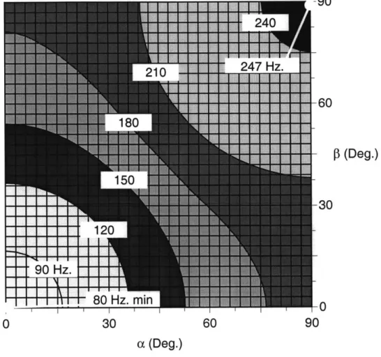
Fundamental frequency versus lay-up for a free-free cylinder with a [±aI ±/8]s lay-up and no honeycomb withj < 6...86

Second frequency versus lay-up for a free-free cylinder with a

[±aI ±/]s lay-up and no honeycomb withj < 6... 87 Fundamental frequency versus lay-up for a free-free cylinder with a

[±a/ ±/s lay-up and 0.635 cm (0.25") thick honeycomb withj < 6 ... 88 Fundamental frequency versus lay-up for a free-free cylinder with a

[±l ±#/]s lay-up and 1.91 cm (0.75") thick honeycomb withj < 6 ... 89 Second frequency versus lay-up for a free-free cylinder with a

[±a/ ±3s lay-up and 1.91 cm (0.75") thick honeycomb with j < 6 ... 90 Frequency versus honeycomb thickness for a [02 / ±47]s lay-up for

0 < j < 5, N = 10 ... 91 Frequency versus honeycomb thickness for a [02 / ±47]s lay-up for

first three extension modes, j= 0, N = 10 ... 92 Frequency versus honeycomb thickness for a [02/ ±47]s lay-up for

first three torsion modes, j= 0, N = 10... 93 Six lowest frequencies for a [0 / ±47 / O]s lay-up, with a honeycomb thickness of 1.91 cm (%") including through thickness

shearing,

j

thickness of 1.91 cm (%") for approximate analysis, N= 10,

j

Standard deviation of the CTE in the x direction versus lay-up for a

[± a / ± 3 s lay-up ... 10 1 Standard deviation of the CTE in the x direction versus lay-up for

zero CTE lay-ups in the [± l ±a/ s family ... 102 Problems encountered during cylinder manufacture ... 104 C ylin d er 3 ... 10 6 Illustration of the flatwise tension rig and specimen... 119 Load versus stroke for the second flatwise tension test ... 120

Figure 6.3: Figure 6.4: Figure 6.5: Figure 6.6: Figure B.1: Figure C.1: Figure D.1: Figure E.1: Figure E.2: Figure E.3: Figure E.4: Figure E.5: Figure E.6: Figure F.1: Figure F.2: Figure F.3: Figure F.4: Figure F.5: Figure F.6:

Longitudinal stress versus longitudinal strain for specimen Al ... 123

Longitudinal stress versus transverse strain for specimen Al... 124

Coefficient of thermal expansion for a [0 / ±47 / 0]s laminate not therm ocycled ... 129

Coefficient of thermal expansion for a [0 / ±47 / 0]s laminate thermocycled between 93.3"C and -129"C (±200"F) for 50 cycles ... 130

Geometry and coordinate system of lateral strength model ... 157

Frequency versus number of assumed modes, N, for a [02 / ±47]s lay-up with 1.91 cm (0.75") thick honeycomb forj > 0... 170

Determinate of Bc versus the radial frequency for a cylinder with

j

Illustration of the telescope tube mandrel ... 185

Illustration of the lay-up table with the mandrel ... 187

Illustration of the telescope tube end rings... 189

Illustration of the telescope tube cutting jig ... 191

41 C ure cycle for A S4/3501-6 ... 214

Example of core crushing and dimpling in Plate 1 ... 219

Illustration of core crushing and dimpling in cylinders... 221

Plate w ith collapsed core ... 223

Wrinkling due to poor adhesion at core splice in Shell 1... 227

Illustration of facesheet for cylinder 1 and ring 3... 232

Figure F.7:

Figure F.8:

Figure F.9:

TELAC and the bagging method for all ring and cylinder cures after cylin der 1...239 Illustration of the fiberglass tab used in an attempt to reduce

wrinkling due to the top sheet for Ring 2... 246 Cylinder deformation modes due to the application of pressure

durin g curin g ... 24 8 Figure F.10: Mechanically fastened top sheet for cylinder 2... 250

TABLE OF TABLES

Table 2.1: Small-Sat design overview ... 25

Table 2.2: Small-Sat numerical structural design parameters ... 28

Table 4.1: _{TELAC AS4/3501-6 35% Gr/E material data... 64}

Table 4.2: Hexel Flexcore 5052/F40-0.0025 4.1 pcf material properties... 65

Table 4.3: Cytec FM 300M adhesive film 0.03 lbs/ft2 _{material properties ... 67}

Table 4.4: Thermal Analysis Input Parameters ... 69

Table 4.5: Comparison of closed form frequencies with approximate frequencies... . 98

Table 4.6: Probabilistic analysis input parameters ... 100

Table 5.1: Manufacturing problems addressed by various specimen g eo m etries ... 10 9 Table 5.2: Manufacturing problems and solutions ... 110

Table 5.3: Estimation of time to manufacture one cylinder ... 114

Table 5.4: Specimens manufactured for testing ... 116

Table 6.1: Flatwise tension failure load and stress for the specimens tested ... 121

T able 6.2: T ensile test data... 125

Table 6.3: Tensile test data, continued ... 126

Table 7.1: _{MCLAM AS4/3501-6 35% Gr/E material data... 142}

Table 7.2: _{Comparison of theoretical and experimental properties with} standard deviations ... 143 Table 7.3: Comparison of design goals and computed values for the Small-Sat

NOMENCLATURE

a Acceleration m/sec2

di Unknown vectors

A Cross-sectional area m2

A y Laminate extensional stiffness N/m

AF Albedo Factor

ei Unknown boundary condition coefficients

C, Specific heat J/K

By Laminate extension-bending coupling stiffness N

Bc Boundary condition matrix

Dj Laminate bending stiffness N m

E Isotropic Young's modulus N/m2

Ei Young's modulus in the i direction N/m 2

F Force N

f

t,

FdA-E View factor between earth and element

FS Factor of safety

g Acceleration due to gravity at sea level m/sec2

G Isotropic shear modulus N/m2

h Cylinder wall thickness m

hk Ply location in a laminate _m

i The square root of -1

I _{Laminate mass moment of inertia per unit area kg}

IYY Area moment of inertia in the y direction m4

j

k Ply index

K Radial conductivity W/m K

Ki Stiffness matrix premultiplying the ith derivative of X

L Cylinder length m

LFxial Axial quasi-static load factor

LFLaterial Lateral quasi-static load factor

m Mass _kg

MX Out of plane traction in the

#i

m0 Out of plane traction in the

#,

M Bending moment N m

M Stress couple in the i direction N

MT Isotropic thermal bending moment N

& T Thermal bending moment vector N

Msat Mass of satellite kg

p Out-of plane traction in the z direction N/m2

Ni Stress resultant in the i direction N/m

N Isotropic thermal stress resultant N/m

[- T Thermal stress resultant vector N/m

4

ge Average earth heating W/ m2

qx In-plane surface traction in the x direction N/m2

q0 In-plane surface traction in the 6 direction N/m2

Qi

Q

Q

Q

Q

R Cylinder mid-plane radius m

So Nominal solar heat flux W/m2

t Time coordinate sec

T Ply transformation matrix

TO Temperature at which optics are calibrated K

T, Maximum temperature K

T2 Minimum temperature K

Mid-plane displacement in the x direction _m m m m Displacement in the 6 direction

Mid-plane displacement in the 0 direction Displacement in the z direction

Displacement vector

Homogenous solution displacement vector Particular solution displacement vector

Derivative of the displacement vector with respect to x Derivative of the homogenous solution

vector

Isotropic coefficient of thermal expansion

displacement m/m0C Xh f P Ph a aA j64

Rotation about the 0 axis Change in temperature

Difference between maximum temperature temperature at which optics are calibrated

Difference between minimum temperature temperature at which optics are calibrated

and and m/m C m/m C m/m m/m OC OC OC V w Solar absorptivity

Coefficient of thermal expansion in the i direction Laminate coefficient of thermal expansion in the direction

Rotation about the x axis

AT AT,

AT2

A TExt Temperate change which causes extension 0C

ATBend Temperate change which causes bending "C

AL In plane displacement due to thermal extension m

AY Out of plane displacement due to thermal bending m

E Emissivity

egi Tensor strain in the ij direction m/m

E 0 Tensor mid-plane strain in the ij direction m/m

Ply angle Deg

K Curvature in the i direction 1/m

A Eigenvalue

e Angular rotation due to thermal bending Rad

Pk Density of kth ply kg/m3

Laminate mass per unit area kg/m2

a Stefan-Boltzmann constant W/m2_K4

Stress in the ij direction N/m2

UMax Maximum stress in the x direction N/m2 v Isotropic Poisson's ratio

Vyi Poisson's ratio in the ij direction

co Radial frequency Rad/sec

SUBSCRIPTS AND COORDINATES

x Cylinder axial coordinate m

y Cylinder coordinate orthogonal to the x and z axes m

z Cylinder through thickness coordinate m

0 Cylinder circumferential coordinate Rad

1 Material axis aligned with the fiber

2 Material axis in plane transverse to the fiber

CHAPTER 1

INTRODUCTION

Satellite structures must survive launch and provide stiffness, dimensional stability, thermal control, and equipment containment and mounting. Current design practice is to have separate structures for each of these functions. This practice is acceptable for large vehicles, but does not scale well. In small vehicles, many of these functions can be met with very little material, resulting in designs dominated by practical manufacturing constraints (minimum gages, tolerances, etc.) rather that the actual requirements. Therefore, the true structural mass fraction (including things such as electronics support racks and boards, radiators and thermal control material, and launch related structures such as cradles and support frames for multiple vehicles) becomes very large in small vehicles.

This represents a problem, but also an opportunity. In general, an examination of the basic physics that sizes such systems is very favorable to small systems. For example, the material required for structural stiffness to achieve desired deflections and vibration frequencies decreases in proportion to a decrease in the structural size raised to the third power. However, for very small vehicles it is difficult to take advantage of these physics because practical considerations such as minimum material gages, joining technology,

and the need for equipment containment and support, limit the use of current designs and design practices. New approaches to the design and integration of primary structure and hardware for functions such as thermal control and equipment mounting are needed. New design concepts, including multifunctional structures, promise to not only solve this problem, but also deliver dramatic weight and cost savings, with simpler and more reliable systems.

This research develops and demonstrates new technology for the design and production of multifunctional mini-satellite structures. The technology is developed through the design, analysis, construction, and testing of a mini-satellite structure. A Charles Stark Draper Laboratory system is used as a baseline. Draper Laboratory, in conjunction with the Massachusetts Institute of Technology, is building a small reflecting telescope that utilizes existing technology to provide ground observation data from low earth orbit, at a minimal cost. The goals of this research are to design, analyze, build and test a flight-worthy multifunctional structure for this satellite. The structure was designed and analyzed taking strength, thermal, optical, vibration, and material probabilistic analysis into consideration. A program was undertaken to manufacture sample flight-worthy components. Flat panels, curved panels, rings and partial tubes were built, culminating in the production of a full sized satellite bus structure. Tests were performed to validate the assumptions used in the design. Testing included flatwise tension testing of bond strength, tensile testing to confirm failure strength, and Coefficient of Thermal Expansion (CTE) verification.

Previous work relevant to the current research is described in Chapter 2. This includes a detailed description of the Draper Small-Sat and issues relevant to the design of a multifunctional structure, and a description of the background of technologies and analysis used in this project. Strength, thermal, optical, and dynamic analysis shall be presented in Chapter 3. Chapter 4 will present the implementation of the analyses presented in Chapter 3. Issues dealing with the manufacture of the structure will be reviewed in Chapter 5. Testing methods and results for the structure will be presented in Chapter 6. The results of the design, analyze, build and test program presented in Chapters 4, 5, and 6 will be analyzed and discussed Chapter 7. Concluding remarks will be presented in Chapter 8. A closed form axial and bending analysis will be presented in Appendix A and B. Appendix C and D will present a simplified and closed form vibration analysis. Cylinder manufacturing instructions are listed in Appendix E. In Appendix F manufacturing problems and their solutions are presented. A list of manufactured specimens for this program will be tabulated in Appendix G.

CHAPTER 2

BACKGROUND

This chapter presents background information on the Draper Small-Sat design, analysis, manufacturing, and testing. Discussion of the major subsystems is presented in the Draper Small-Sat Design Overview. The outline of the structural subsystem is also presented in this section. A brief presentation of the background for the structural, thermal, optical, vibration, and probabilistic analyses are also presented in this chapter.

2.1

DRAPER SMALL-SAT DESIGN OVERVIEW

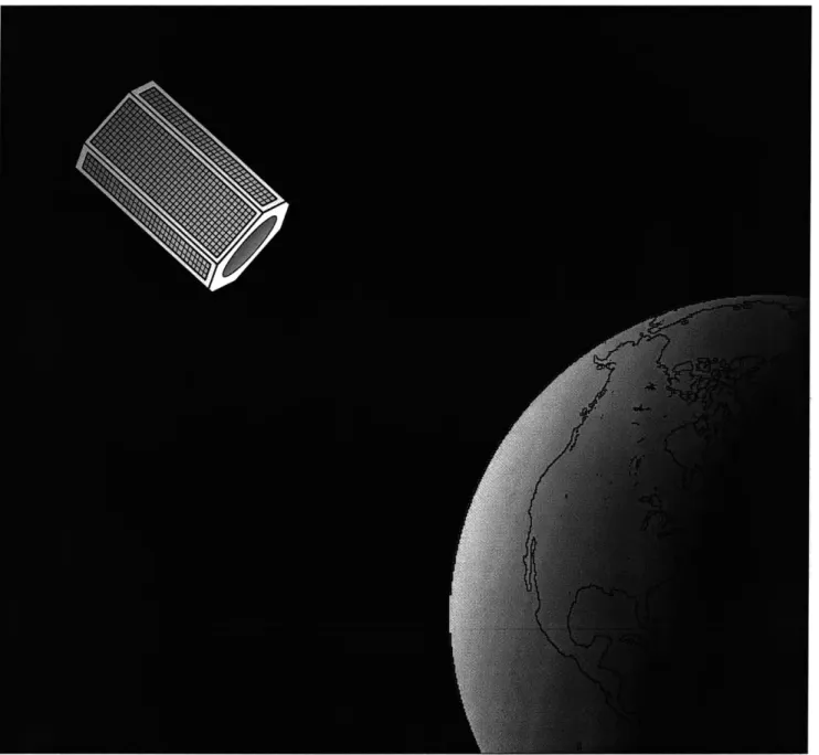
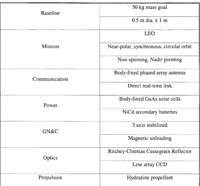
The Charles Stark Draper Laboratory, in conjunction with the Massachusetts Institute of Technology, is building a small reflecting telescope that utilizes existing technology to provide ground observation data from low earth orbit, at a minimal cost. This satellite, known as the Draper Small-Sat, is shown in Figure 2.1. Table 2.1 summarizes the major subsystems of the satellite.

Table 2.1: Small-Sat design overview

50 kg mass goal Baseline

0.5 m dia. x 1 m LEO

Mission Near-polar, synchronous, circular orbit Non-spinning, Nadir pointing Body-fixed phased array antenna Communication

Direct real-time link Body-fixed GaAs solar cells Power

NiCd secondary batteries 3 axis stabilized GN&C

Magnetic unloading

Ritchey-Chretian Cassegrain Reflector Optics

Line array CCD

Two shells were selected for the design of the structure of the satellite, which can be seen in Figure 2.2. The innermost shell is known as telescope tube. The telescope tube is a 1 m (39.4") long graphite/epoxy cylinder with an inner diameter of 40.6 cm (16"). The tube has two major functions. First, it acts as the primary load carrying structure. The Pegasus XL launch vehicle designed by the Orbital Science Corporation was selected as the launch vehicle for the satellite. This tube will be cantilevered off the launch vehicle with all of the satellites internal components connected directly to the telescope tube. This launch vehicle imparts a quasi-static load of 13 g's in the telescope tubes axial direction, and a 9.5 g lateral load factor. The structure was designed to resist first ply failure during the launch. Providing a thermally stable platform for the optics is the second major function of the telescope tube. To prevent the mirrors from displacing relative to each other while undergoing thermal loading in space, the telescope tube has a near zero CTE in the longitudinal direction.

The telescope tube has several other major attributes. First, the telescope tube has a design frequency of 90 Hz to make the structure appear rigid to the stabilization mechanisms. Second, it was hoped by adding a large margin of safety to the strength analysis, the telescope tube would be highly robust so that it would be resistant to accidental damage, and the addition of holes used to mount components. Numerical structural design parameters are listed in Table 2.2.

Solar Panel Structure

Telescope Tube

Optics and CCD

Figure 2.2: Draper Small-Sat internal lay-out

~1

I I

I I

I I

Table 2.2: Small-Sat numerical structural design parameters

Property Value

Satellite mass 50 kg

Structure mass goal 10 kg

Satellite length 1 m

Telescope tube inner diameter 0.406 m

Minimum structural fundamental frequency 90 Hz.

The second shell is known as the solar panel structure. The solar panel structure has three functions: it provides a mounting platform for the solar panels, it provides an area in which a radiator could be added, and it provides thermal shielding for the internal structure. The solar panel structure is an octagonal structure on which GaAs solar cells will be mounted. The solar panel structure needs to be rigid enough to prevent damage to the solar cells under inertial and thermal loads. The sides of the solar panel structure that have no solar cells act as radiators for the satellite. The solar panel structure also acts as a shade, and to a lesser extent, to transfer heat around the telescope tube, thereby suppressing bending of the telescope tube.

The design, analysis, manufacturing, and testing of the telescope tube has been the primary focus of this work. The design and analysis of the solar panel structure has not gone beyond the preliminary stages. It is felt that any knowledge gained by designing, analyzing, manufacturing, and testing the telescope tube could be easily transfer to the solar panel structure. The structure required to connect the two structures also has not been designed. Issues for designing the connecting structure are maximizing load transfer of the solar panel structure to the telescope tube during launch, minimizing thermal transfer between the solar panel structure and telescope tube, and vibration isolation of the telescope tube from the solar panel structure. These issues have not yet been addressed.

2.2

ANALYSIS AND DESIGN BACKGROUND

The telescope tube was designed, analyzed, and optimized taking strength, thermal, optical, vibration, and material probabilistic analysis into consideration. The stress in a thin orthotropic tube was derived using the classical thin shell theory equilibrium equations. Using this stress analysis and the Tsai-Wu failure theory, the margins of safety could be determined. Graduate student Yool Kim provided the thermal analysis for an infinitely long tube under static and transient thermal loads. Beam analysis was used to determine the displacement of the telescope tube under the thermal loads. This thermal-deformation analysis was used in conjunction with an optical analysis performed by Draper Laboratory to determine the maximum allowable CTE of the telescope tube to prevent significant defocusing of the optics. Two analyses were used to determine the modes and mode shapes of the telescope tube. The first was a Ritz analysis to determine the approximate modes and mode shapes of the telescope tube. The second analysis is a numerical solution of the equations of equilibrium for an orthotropic cylinder including transverse shearing. The effect of material variation on laminate properties was determined by using an analysis performed by Doctor Hugh McManus.

CHAPTER 3

THEORY

This chapter presents the theory used to design the structure for the Draper Small-Sat. Presented are the Small-Sat structural analysis overview, classical thin cylinder theory, strength analysis, vibration analysis, coefficient of thermal expansion analysis, probabilistic analysis, and a thermal/structural/optical analysis. The global structural design methodology will be presented first in order for the reader to understand the relevance of the individual analyses, and how the analyses all tie together. Classical thin cylinder theory is presented next to define important relations that will be used in subsequent analyses. For optimal performance of the telescope, it is desirable for the mirrors to not deform under thermal loading. To determine the effect of thermal loads on the optical performance of the telescope, a thermal/structural/optical analysis was performed to determine the maximum axial coefficient of thermal expansion (CTE) allowable to prevent defocusing of the optics. Using this CTE, the candidate lay-ups were selected using classical laminated plate theory. To insure that the satellite does not fail due to inertial loads during launch, a strength analysis was done using classical thin cylinder theory and using a Tsai-Wu failure criterion. It is desirable that the satellite

appears rigid to the control subsystem. To insure this, two vibration analyses were performed to determine the modes and mode shapes of the telescope tube.

3.1

DRAPER

SMALL-SAT

STRUCTURAL

ANALYSIS

OVERVIEW

The goal of the structural analysis was to determine a lay-up and a honeycomb thickness that would meet all the design requirements. These requirements included the prevention of defocusing of the optics, building a "stiff' and "robust" structure, and building a structure that is the minimally susceptible to manufacturing variations. The facesheet lay-ups were selected for mass, CTE, strength, and freedom from excessive manufacturing variations. The honeycomb was selected to satisfy stiffness requirements. Both the honeycomb thickness and the facesheet lay-up were selected using an optimization procedure.

To prevent the optics from defocusing, the CTE in the axial direction of the telescope cylinder should be minimized. Knowing the bounds on the thermal expansion in the axial direction decreased the possible pool of candidate laminates. A steady state temperature loading was determined for the cylinder. Using this temperature loading, the deformation of the cylinder could be determined as a function of the axial CTE. Draper performed an optical analysis using a ray trace code to determine the Strell' number as a function of mirror displacement. Assuming a minimum desired Strell number allowed the required axial CTE to be determined. This gave a pool of desirable lay-ups for the telescope cylinder. Using a computer code, the lay-ups that were susceptible to

manufacturing variations were discarded. Many lay-ups were also discarded because they required excessive numbers of plies, and would cause the satellite structure to be too massive. Strength of the satellite was not a constraining requirement because first ply failure was calculated to not occur for the telescope cylinder due to the launch loads, even when a very high factor of safety was used to assure damage tolerance.

A vibration code was used to determine the effect of the honeycomb core thickness on the fundamental frequency. A honeycomb thickness and density were selected to increase the fundamental frequency to a desired value. The lay-up and honeycomb thickness that yielded the least massive solution, with the lowest CTE and CTE variation, and which met all the other requirements, was the candidate lay-up.

3.2

CLASSICAL THIN CYLINDER THEORY

It is generally agreed that a cylinder is considered "thin" if its radius to thickness (R/h) ratio is greater than 202. A "thin" cylinder is assumed to be in a condition of plane stress, that is there is no stress through the thickness of the cylinder. It is also generally agreed that cylinder is considered "thick" if its radius to thickness (R/h) ratio is less than five. In this regime there is unequivocally a stress dependence on the through thickness dimension. There is no clear distinction as to when the stress dependence can be ignored, and when it must be included. Throughout this research cylinders were considered with a radius to thickness ratio of greater than 10. The majority of the cylinder thickness was comprised of very low load bearing honeycomb. It was decided for this research to

ignore the through thickness stresses to simplify calculations. All structural properties will be therefore analyzed with classical thin cylinder theory.

Classical thin cylinder theory is the cylindrical counterpart to classical thin plate theory. In both theories it is assumed that the thickness is much smaller that the other dimensions (h << R, h << L), and there exists a state of plane stress. Consider an infinitesimal element of a cylinder shown in Figure 3.1. The x, 0 and z axis are the structural axis shown in Figure 3.2. The 1, 2 and 3 axis are aligned with the material axis of the lamina, where the 1 axis is in the direction of the fibers. These two axis systems are separated by an angle

#.

I

0 12 JxL

'11 -Cxx

1622[ =

[T]

L₁₂ ELXO

where T is the transformation matrix:

m2 n2 2 m n

[T]= n2 m2 -2 m n (3.3)

-m n m n m2 _n2

where m = Cos(#) and n = Sin(#) in the transformation matrix. It should be noted that all strains are tensor strains in the above transformations. Using Hooke's law, and assuming plane stress in the 3 direction, in-plane stress and strain can be related for a ply by:

z, 3

0

0::

1

Coordinate system for infinitesimal cylindrical element

2

x

Z

Figure 3.2: 0

Lpp

Coordinate system for cylinder

R

C-1 [E -a, AT

-22

Q=[]

612 2 eCn

Q,

Ol Q12 0~

[Q]= Q12 Q22 0 (3.5)

0 0 Q66

and a are the ply coefficients of thermal expansion in the i direction and Qj are the ply stiffness components. To determine the stresses in the ply in the xOz coordinate system equation 3.4 is transformed to yield:

-E, e- -a, AT o - -ao AT (3.6) 2 EO - axo AT

(]=(T

][

[Q]

(Q)=Q

j

The coefficients of thermal expansion, ax, a, axo, will be defined in Equation 3.22. If it assumed that the dimensions of the cylinder are much greater than the thickness, (h << R, h << L) then the displacement field for the cylinder can be written as:

u = uv (x,6, t)+ z# 9(x,6, t) (3.9)

w = w(x,0, t)

where u, v, and w are the displacements of the cylinder in the x, 0, and z direction, and uO,

vo, and w are midplane displacements.

Qx

Q,

displacement relations for a thin cylinder can be found. The tensor linear thin shell strain-deformation relations5_{, including transverse thickness shear deformation can be}

written as: du0 O = 4o (3.12) dx w) E -dw-₀ " dz d x 1 d3₀ K9 R d O KxO dx/1 + X2 _dx 1 du R dO) (3.13) (3.14) (3.15) (3.16) (3.17) (3.18) 1 d 8x R dO (3.11) E40 = Ido+ R (dO

1' dw 1, =__$_+ (3.19) 2 d x 18 1 dw v( 8,=-# R----

(3.20)

where the 0 superscript denotes midplane strains. The strain displacement relations for a rectangular plate can be derived from the above equations by replacing R d0 with dy and R with infinity in the above equations.

Consider a laminate that is made of n plies stacked one on top of another. If one assumes that the stress in each ply is negligible in the z direction then equation 3.6 for the

kth ply can be written as:

'1- ex+ zK-ax AT

1

J

jaI

Figure 3.3 is a picture of an infinitesimal piece of a laminate. It shows the nomenclature of the stacking sequence of the laminate. The stress in the plies is integrated through the thickness to define the stress resultants, N , and moment resultants, M , and transverse shear resultants Q.

Nomenclature of the laminate stacking sequence

Z

h _x

+h/2

NO =h/2 agf dz

I.

07X

+h/2

M 0 = h12

}oo

Substituting equation 3.21 in to equation 3.23 yields:

K X

2 K

g

ax

zdz -Q AT dz (3.25)

kL

a,J

Substituting equation 3.21 in to equation 3.24 yields:

KXX ax

dz +(Q Iko OI kZ 2 dz -(IQk ao

h-2 icxo _axo

-ATz dz (3.26)

With these two equations the stress strain and moment curvature relations for a thin laminated cylindrical shell are given as:

N₉ No N 0 M, MO 'M e

A

A

In the above equations, the T superscript represents thermal forces. A, B, and are given as: (3.23) (3.24) N ₁ No INXe n k =1

{

I

I

(Q

n

Ah )k(k-hkl) - h(OJ (3.28)

Bin h- hk_)(3.29)

Di h h _) (3.30)

and the thermal line forces, N and M , are given as:

n hk NT _{f (Q)k(aj)kAT dz (3.31)} k=1 _{hk_1} k hk M[ = f ( j)k(aU)kAT zdz (3.32) k=1 hk-I

where i, j are equal to 1, 2, and 6.

For a symmetric lay-up, if it is assumed at a point that the temperature is constant across the thickness of the cylinder, and no external loads are applied at that point, then equation 3.27 can be written as:

{Nl

T

246

N At A 2 A6 10x

NO= A2 A22 2 A26 - (3.33)

J LA6

K (x,0,t ) = KO(x,0,t ) = K,(x,0,t ) =0 (3.34)

If it assumed that material properties are independent of temperature, then equation 3.33 can be written as:

E 1 AT

E0 >= O AT (3.35)

where: ax Io 2 axo = A-r []kI a 2 aO Jk

(hk

Determination of the zero CTE lay-ups will be described in detail in Chapter 4. It should be noted the displacement field for a cylinder with no external loads is given by:

u0(x,9,t)= a AT x

w(x,0, t)= o AT R

(3.37) (3.38) (3.39) In a manner similar to the in-plane stresses, the transverse shear stresses can be related to transverse shear strains by:

{U23

Equation 3.40 can be transformed from the 123 coordinate system to the xOz coordinate system by:

{-23

(E23

#ix(x,

#0

where m = Cos(#) and n = Sin(#). Using equations 3.41 and 3.42, equation 3.40 can be written as:

(

a1Vz _045 Q55 2 Exz

J

It is assumed that the transverse shear stresses are distributed parabolically across the laminate thickness, as is true with shear stresses in the isotropic case. With this assumption, some authors6 have written the shear resultants as

fQ1

= Jh/ 2 XZ dz (3.44)

QO

Qx

{~;}L~

Z

{~}(3.45)

O

where

5 n-,\ 4

A= Q h -h3

(h

)

where i,

j=

Significant simplification of the stress strain and moment curvature relations can be made for various lay-ups. If the material is symmetric through the thickness then

By = 0 and the inplane and out-of-plane line forces are decoupled. If the material is balanced through the thickness then A16 = A26 = 0 and the inplane extension and shear are

decoupled. If the cylinder is composed of a single layer of material aligned with the structural axes, then A16 = A2 6 = D16 = D26 = A4 5 = 0, and B0 = 0. A cylinder with this

configuration is known as specially orthotropic. Some cross ply lay-ups are specially orthotropic and many lay-ups are very close to being specially orthotropic. A specially orthotropic cylinder has a special property of decoupling the displacement modes in the circumferential direction. To simply analysis, all cylinders analyzed were assumed to be specially orthotropic.

Using the above stress strain relations and strain displacement relations and the minimal value of the total potential energy, the linear equilibrium equations for a cylindrical shell can be derived:

dN 1 dN d2 _{u d} 2₂₃ X+ '=q +p ₂0+Q '(.7 dx R d0O dt2 dt2 dN~ 1 dN9

Q

Q

where qx, q, p, mx, and m , are the surface tractions which are functions of x and 0. It should be noted that each surface traction corresponds to a displacement, for example qx with uo and p with w, and the traction and that displacement have the same positive direction. The surface tractions are defined as9:

q x = h12 Zx /hi2 GO = ooh1₂ G Zj -h/2 P = h/2 0ZZ1-hI2 MX = h Qxh/2 + Zx -h/2) h MO = 2(0Z1h/2 + -hO /2 (3.52) (3.53) (3.54) (3.55) (3.56)

)

The mass terms in equations 3.47 -3.51 for a n ply laminate can be defined as

1-n hk

Q=pJ

where pK is the density of the kth ply, and h is defined in Figure 3.3. If the mass distribution in the laminate is symmetric then

Q

x = 0 and x = L Either u = 0 or N, =0 Either v =0 or N,,= 0 Either w = 0 orQx =0 (3.60) (3.61) (3.62)

Either/#x = 0 or Mx =0 (

Either/#, =0 or Mx = 0 (3.64)

The equations of equilibrium, strain displacement relations, and stress strain relations for a specially orthotropic cylinder shall be used throughout the structural analysis. All lay-ups considered will be balanced and symmetric, therefore

A1 6 = A2 6 = Byj = 0. Analysis which solve the equations of equilibrium will make an

assumption that D1 6 = D26 = A4 5 = 0 in order to decouple solution modes.

3.3

THERMAL/STRUCTURAL/OPTICAL ANALYSIS

3.3.1 Thermal Analysis

The thermal response of a tubular structure in various orbital positions was determined using the analytical methods derived by Yool Kim'1. In this analysis, it was assumed that the cylinder was infinitely long, and therefore the temperature is only a function of the circumferential direction. Using conservation of energy, the equation that governs the thermal response of an infinitely long cylinder can be derived:

~~ 3 T k hi 32 T

p CTt - - e T4 +Q,t,+Q flV (3.65)

a t R T30

where Qint is the energy due to internal heat generation, and

Q,,n

After many orbits, the satellite's temperature profile reaches a cyclic steady state. For a differential element of the cylinder, equation 3.65 can be written as":

a

()4 +-r 4 4

-p Cp h + 2 2 6 - Sin(-j (T(V) T-T(O) d

a t R 364 f 2

+aA So0 +E q, FdA-E+aA AF So _{FdA-E COS(0)}

(3.66) where for this equation:

Cos(0) -- <

<-o

0 - < 0<

2 2

The terms in equation 3.65 represent in order the heat change due to: the transient response, the conductivity, the thermal radiation emanating from the outside of the satellite, the internal thermal radiation, the solar heat flux, the earth heat flux, and heat flux due to the earth's albedo. Recasting equation 3.66 into finite difference form, the unknown temperature can be solved for as a function of position and external heating. Two analyses were carried out. First, a steady state thermal analysis was preformed where the transient term was ignored, and the pseudo steady state temperatures at a number of orbital positions were calculated. Orbital positions entered the calculations via values of So (solar heat flux) and FdA-E (view factor of the satellite to earth). Worst-case

values of T, (maximum temperature) and T2 (minimum temperature) were taken from this

analysis. These calculations were repeated for various values of thermal mass (C, p h). The second set of analyses included thermal storage they were begun at an arbitrary initial

position and continued until the history of temperatures through one orbit resembled the previous orbit to within a small factor. The vehicle was assumed to be in a single orbit that was expressed in equation 3.65 by values of So and the view factor that changed throughout the orbit. Again, worst-case values of T, and T2 were extracted.

3.3.2 Thermal Deformation Analysis

The thermal states calculated using the thermal analysis were incorporated in a simple thermal deformation model to calculate (i) the change in length of the structure due to the change in the average temperature of the structure from the temperature at which the optics was calibrated, and (ii) the bending distortion of the structure. The telescope tube is modeled as a simple beam with a circular cross section and the temperature is assumed to vary linearly in the cross section. Thus, both of these cases are stress free (on a global level, not on a ply level), and deformations can be calculated directly by integrating the thermal strains. If To is the temperature at which the optics are calibrated, and T, > T2 and T, is assumed to be on the opposite side of the cylinder from

T2 (which in practice is the case) then the change in temperature on either side is given by:

AT = T - TO (3.68)

AT2 = T2 -T (3.69)

These changes in temperature can be transformed into a change in temperature that causes extension and one that causes bending of the beam:

= AT,+AT T+T

ATExt 2 _ I+2 _ TO (3'70)

2 2

ATBend =AT - AT=T -T ₂ (3.71)

If is assumed that the beam undergoes stress free deformation, and through thickness shear strains are neglected, then using only geometric considerations the thermal deformations can be found. The angular difference between the midplane of the beam and the tip, as shown in Figure 3.4, is given by:

L a

E =- ATBed (3.72)

4R

where a is the longitudinal CTE, and L for this analysis is the half length of the telescope tube. The displacement of the tip is given by:

AY = 2 R

(1-

(E))I±aAT

KATBend

The axial displacement of the beam is:

AL=2RSin(E)K 1+aATxt L (374)

aATBnd 2

The above three equations do not assume small angle deformations. If it is assumed that the angular tip displacement is small then the following approximations can be made:

AY ~ (a ATBend 2 ATBd ATExt) (3.75)

4

AL = LaATExt (3.76)

The second term in equation 3.75 represents the extension-bending coupling. The coupling term proved to be inconsequential for the configurations considered.

AL --- +

i L

----T 2-- - - - -

---AY

Deflection of the satellite cylinder under a thermal load Figure 3.4:

Neglecting this term reduces equations 3.75 and 3.76 to the familiar form describing the thermal deformation of beams. Note the analysis has been developed for a cantilevered structure. An unsupported (free-free) structure can be analyzed as two identical cantilevered structures by assuming symmetry about the centerline.

3.3.3 Optical Analysis

One of the functions of the structure is to support telescope optics. The primary mirror is supported near the middle of the structure, and the secondary mirror supported at one end, as shown in Figure 2.2. The thermal deformations cause a change in distance and angular orientation between the two mirrors resulting in degradation in performance of the telescope. The calculation of this optical degradation was done at Draper Laboratories. For a given length change AL, and angular misalignment 0, a ray tracing routine was used to calculate the Strell number, a metric of the image quality'.

A Strell number of 1.0 represents a perfect telescope. A maximum Strell number of 0.977 can be achieved with the desired aperture and focal length of this telescope assuming no misalignment of the mirrors due to deformation. For various sets of length changes and angular misalignments, the Strell number was calculated. Equations 3.72 and 3.76 relate the temperatures, geometry, and CTE to these deformations. For a known temperature state and geometry, the CTE required to achieve the desired Strell number can be determined.

3.4

PROBABILISTIC ANALYSIS

Using a methodology devised to determine the standard deviation of laminate engineering properties from the standard deviations of ply properties , the standard deviation of the CTE in the x direction can be used a figure of merit to determine the relative worth of two nominally zero CTE lay-ups. For example, if two lay-ups are compared, the lay-up with the lower standard deviation is more desirable because it is less susceptible to random manufacturing variations. This analysis was used to weed out undesirable lay-ups from the design space. This analysis assumes that the laminate CTE is a function of independent normally distributed ply properties: ply thickness, stiffness, Poisson's ratio, and CTEs. The standard deviation of the coefficient of thermal expansion in the x direction is given by:

2

2x _(3.77)

where in the above equation ai is the standard deviation of i, and Xi is the ith independent variable. Details of the input parameters used for this analysis will be presented in Chapter 4.

3.5

STRENGTH ANALYSIS

The Small-Sat will undergo the greatest loading during launch. For preliminary design purposes, it was assumed that the inertial loading was quasi-static. It was also assumed for preliminary design purposes that the mass of the components was evenly