The development of an interactive graphical risk analysis system

ALFRED

SLOAN SCHOOL

OF

MANAGEMENT

THE DEVELOPMENT OF AN

INTERACTIVE GRAPHICAL RISK ANALYSIS SYSTEM James Beville-John H. T«Jagner Zenon S. Zannetos December, 1970 502-70

MASSACHUSETTS

INSTITUTE

OF

TECHNOLOGY

MEMORIAL

DRIVE

BRIDGE,

MASSACHUSETTS

DtV^'EYLIBRARY

THE DEVELOPMENT OF AN

INTERACTIVE GRAPHICAL RISK

ANALYSIS SYSTEM

James Beville

John H. Wagner

Zenon S. Zannetos

December, 1970

--

This paper is part of a continuing research effort of the Managerial

Information for Planning and Control Group at the Sloan School of

Management at M.I.T. . The support of the Army Material Command, the Land

Education Development Grant, NASA, and the I.B.M. Grant to M.I.T. for

RECEIVED

JAN

26

I. INTRODUCTICfN

One of the most elusive problems faced by management today is

that of imposing structure on the decision-making process when

operating in an environment characterized by substantial uncertainty.

For example, when managers make decisions relating to activities such

as capital budgeting, choice of pricing strategies, new product

develop-ment, aquisitions, or mergers, they must somehow cope with the

uncertainty inherent in these problem areas. Hertz (1) notes that the

causes of the difficulties with these types of decision lie not in the

problem of projecting the expected return for a particular course of

action, given a set of assumptions, but in the assumptions themselves and

in accessing their impact on the decision. The reasoning is that while

each assumption has associated with it a degree of uncertainty which

singly may be manageable and possibly palatable, when taken together the

combined uncertainties can induce an uncertainty of critical proportions.

When operating in a decision environment characterized by the

aforementioned type of difficulty, assumptions in the form of point

estimates for variables such as market share, industry sales volume, etc.,

cannot be taken as factual, but must be viewed in light of the risk

involved in actually attaining them. Thus the decision maker, in

arriving at a decision must develop some form of a risk measure for

each alternative under consideration and perform some form of a trade

off between expected return and uncertainty. Typically, the decision

maker's approach might be to, (1) be overly conservative in estimating

return on investment, (2) rely on the judgement of subordinates who have

a good record for making estimates, or (3) require riskier alternatives

- 2

-to meet higher criteria. Although such approaches have worked in

the past, and will no doubt continue to be used in the future, for

decisions which might have an important impact on the long-term

profitability of the firm, a more rigorous approach to decision making

would seem reasonable, especially since some methodology and tools are

available for this purpose.

This paper describes the efforts of the Managerial Information

for Planning and Control Group at the Sloan School of Management,

Massachusetts Institute of Technology, during the 1969-1970 school

year, to apply management science techniques and computer technology to

this general decision-making environment. Specifically our work has

focused on the use of risk analysis models and computer-driven interactive

visual display devices as the major components of a management decision

system. And this in order to aid the decision maker by providing him

with both a framework for decision making and a means for implementing

II. RISK ANALYSIS NODELS

In general, the objective of risk analysis models is to provide

structure to the problem environment by identifying the basic components

of risk and assigning to each of these components probability measures

for all possible outcomes. For example, for a typical business decision,

the basic elements of revenues and expenditures would be first identified,

then for those elements for which uncertainty is greatest further

sub-divisions would be made until all critical elements of the environment

had been identified to the level that it is possible to specify possible

ranges of outcomes and their associated probabilities of occurrence.

Figure I gives a possible risk model structure for a new product decision.

For each element so identified, a probability distribution describing

all possible outcome states must be developed.

Figure I

Structure for a Risk Analysis Model

For a New Product Decision

Net

Income-Expenditures.

-Revenue

Research

Marketing

-Industry Volume

•Market Share

-Price Per Unit

- 4

-Once all of the outcome states for each of the elements of

risk have been described in the form of probability distributions,

these distributions can be aggregated by means of a Monte Carlo type

process to develop a probability distribution describing the expected

net return for the alternative being modeled.

As we have already mentioned, risk analysis models provide both

a framework for structuring decision alternatives, through the

identification of the elements of risk in a hierarchical manner, and

a methodology for analytically dealing with risk, through the use of

probability distributions and the Monte Carlo simulation. On the

negative side, however, associated with the use of risk analysis

models are the heavy computational requirements posed by the use of

the Monte Carlo process, and the problem of the development of the

probability distributions required to define the basic elements of

risk.

III. INTERACTIVE VISUAL DISPLAY DEVICES

The application of computer-driven interactive visual display

devices to the management setting is currently in its initial phases.

Some characteristics of systems based on such devices which have the

potential for having an important impact on the management decision

making process have already been identified by Morton (2,3). These

characteristics include:

1. Rapid manipulation of data through computer processing in

- 5

-2. Graphical presentation of data which, work by Morton (2,3)

indicates, can be of great value in helping the decision

maker to identify relationships and trends. This characteristic

appears to be especially applicable to the problem of working

with probability distributions, if the assumption can be

validated that people conceptualize probability distributions

better in a graphic rather than in tabular form.

3. Rapid, yet simple, system user interactions through devices such

as light pens. This feature appears to be particularly applicable

to the problem of working with probability distributions in that

it provides a means for rapidly entering such distributions to

models by simply drawing them on the terminal screen with a

light pen. The latter also provides a simple means for

interacting with the computer system through the initiation of

a command by simply pointing to it with the pen.

4. Fast and quiet operation. Such devices are quiet and much faster

than computer-driven teletype terminals. On the basis of our

experience the realized speed of visual displays is greater

than that of teletypes by a factor of approximately ten.

5. There is a certain amount of charisma associated with display

devices which increases the decision maker's willingness to

use them (Morton 2,3).

IV. RESEARCH PHILOSOPHY

display devices indicate that these techniques could provide the

basic components for a management decision system directed towards

problem environments characterized as unstructured and harboring

uncertainty. The risk-analysis model provides a structuring

frame-work and a methodology for analytically dealing with risk, while

the computer-driven interactive visual display device provides not

only the computational power needed to run the models but also the

interface between the decision maker and the modeled situation.

Realizing that managers have reservations toward the use of computers

in decision making and that very little has been done in the past

to determine the impact of interactive systems on the quality of

decisions and on managerial styles, we set as the objective of the

research reported here to investigate some dimension of these

questions using as a research vehicle a managfiment decision system

based on a risk-analysis model and a computer-driven interactive

visual display device.

To attain the aforementioned objectives a methodology was

developed which called for the design, development, and implementation

of a prototype system. There are several reasons for selecting this

research strategy over a purely conceptual study or simulated experiments

void of an actual operating system. First, there is insufficient

theoretical work available to use it as the sole basis for accessing

the managerial implications of the decision-making concept we are

investigating. Secondly, it was felt that the use of simulated

experiments void of an operational system would require too many

- 7

-applicability of the experimental results to actual systems. Thirdly,

it was felt, that in addition to the benefits derived from using a

prototype system as an experimental testing device, the actual process

of designing, developing and implementing a prototype system would provide

us with data relative to the costs and problems associated with the

development of systems of this type.

V. DESIGN PHILOSOPHY

The basic philosophy used in the design of the system was that

the system should be as flexible and as generalized as possible to

allow for its application to different problem environments. That is,

we were interested in the development of a generalized decision-making

tool rather than a device to aid in the solution of one specific

problem. We of course realized at the outset that substantial

progress in system design comes, more often than not, after a primitive

prototype is developed and used as a basis for subsequent iterations.

In order that the latter occur, however, flexibility for subsequent

adaptations must be among the design objectives of the prototype,

otherwise one will have a dead-end system.

The particular operational assumptions underlying the design

decision were the following:

1. For economic justifiability, the system must have the

capability to use the same basic system core and with only

limited additional resources be adaptable to specific problems.

2. There is a need for flexibility so that the system can

be adapted to suit the decision-making style of the individual

3. The system must be viewed as an integral part of a

generalized decision-making framework and be capable to

respond to particular problem environments.

Simon's (6,7) decision-making framework was selected as the basis

for the system design because of its wide acceptability. Simon's

framework is based on an iterative process composed of three phases

--an intelligence, or problem searching phase, a design in which

alternative problem solutions are developed, and a choice phase in

which a course of action is selected.

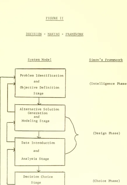
Figure II shows the model of the decision-making process we

developed, based on Simon's framework, which served as the basis for

our prototype management decision system.

As seen in Figure II, the decision process is viewed as consisting

of four stages and being iterative in nature. By iterative it is meant

that the process of operating on one stage will tend to generate ideas

or concepts which will have implications for the other stages in the

process, and when this occurs the stages which are implicated are revisited

and reviewed.

The first stage of this process is referred to as the problem

Identification and Objective Definition phase and is analogous to

Simon's intelligence phase. During this stage, the decision maker

defines the problem, specifies its scope, explicitly states those

assumptions he wishes to use in the decision-making process, and the

criteria which are to be used for evaluating alternative problem

solutions

- 9

FIGURE II

DECISION - MAKING - FRAMEWORK

System Model Simon's Framework

Problem Identification and Objective Definition Stage :i^ Alternative Solution Generation and Modeling Stage Ui^ Data Introduction and Analysis Stage Decision Choice Stage (Intelligence Phase) (Design Phase) (Choice Phase)

- 10

-The second stage of the decision-making process is directed

toward the development of a procedure for problem solution.

Specifically, this stage consists of a method for generating

alternative solutions and developing the general risk analysis

model structure for each of the possible problem solutions. That is,

for each possible solution, a model structure is developed which

identifies all key elements of the solution and the relationships

between these elements.

The third stage is the Data Introduction and Analysis Stage. This

stage together with the previous one represents Simon's design phase

in his decision-making framework. During this stage, data are entered

to the models developed for each of the possible solutions being

analyzed as defined in the second stage. Data which are entered to

these models are of two types: (a) values of the variables which are

used in the equations which define the relationships between elements

in the risk model, and (b) subjective probability distributions which

are used to define the possible outcomes for the independent elements

of the model.

The analysis portion of this stage is based on running the

alternative models, observing the results along the dimensions

established in the first stage as criteria for evaluation, making

desired adjustments in the input data and observing the impact on the

outputs of the model to simulate possible changes in the environment.

The fourth and final stage consists of arriving at the actual

decision as to which alternative course of action to take, and is

- 11

on the observed output of each of the model runs and the particular

decision maker's utility function for return versus risk.

As previously pointed out, this entire process is viewed as

iterative in nature and thus many passes through this process might

be made before a final decision is reached. The actual hardware/

software system with the man/machine interactions used to implement

this decision-making process is what we refer to as a management

decision system.

VI. GENERAL SYSTEM DESIGN

To implement the proposed decision-making system a number of

design objectives, some of which later on will be classified as

hypotheses for testing, were established.

1. Interactive. In order to optimize the decision maker's

time and also provide flexibility for changes, it appeared advantageous

to provide an interactive capability to the decision maker during

the Data Introduction and Analysis Stage of the decision-making

process. It is during these stages that the manipulative capabilities

of the system are required and also the greatest call for the

application of the decision-maker's judgement is made. During these

stages, it is highly desirable for the decision maker to be able to

formulate new hypotheses relative to the input data and immediately test

the effect of such on the outcome of the model.

It was felt that for the initial system and in view of the added

12

for placing the alternative modeling stage of the decision-making

framework in an interactive mode. The following amplify somewhat

further on the reasons which influenced our choice in this respect.

(a) Basic model structures for problem solutions are subject

to much fewer changes during the decision-making process

than changes in the data used in each model. Thus in

attempting to take our first steps, and optimize the

decision maker's time, we felt no pressing need for

placing the Modeling Stage in an interactive mode and

instead concentrated our efforts on the Data Introduction

and Analysis Stage.

(b) The costs involved in placing the Modeling Stage in an

interactive mode would have approximately doubled the

system development costs.

Thus the decision was made to carry out the Alternative Solution

Generation and Modeling Stage in a batch-type mode of computer

operation, in which instructions defining the model structures to

the system are entered in a non-interactive manner using a macro

instruction-type language.

2. Response Time. In order to maintain the decision maker's

span of attention during the interactive mode of operation with the

system, we felt that a real-time response to a user's request was

necessary. We defined "real time" to be any response of less than

15 seconds. There were no time constraints placed on the batch mode,

as the decision maker was not actively involved in the decision-making

- 13

-3. Adaptive. It was hypothesized that as a user became more

familiar with the operation of a system, he would request additional

system options. Thus an adaptive capability was deemed necessary

to allow easy modification of the system to satisfy user requests.

4. Generalized. There was also a need for using risk-analysis

models of different hierarchical forms in order to provide the

manager with the capability to deal with different problem environments.

5. Simple to Use. As the system was primarily directed towards

top management personnel, it was necessary that it be easy to interact

with, and not require the user to learn a programming language, or

an elaborate set of instructions. In addition, the learning period

on how to operate the system had to be short.

6. Graphical Presentation of Data. Since probability

distri-butions were to be the primary format for both input and output data,

graphical presentation of data was critical. To aid in understanding

and developing subjective probability distributions, and because

experience was needed before one could determine which was more relevant,

the dual capability was specified for displaying both cumulative probability

distributions and probability density functions.

7. Modular Design. For ease of development, and to insure an

ability to easily modify the system, a method of decoupling the system

was necessary. A modular design, which allowed the system to be

decomposed into a number of subsystems, each of which could be developed

- 14

VII. DETAILED SYSTEM DESIGN

In line with the objectives specified in the previous section,

the system was designed to facilitate two types of interactions

--problem solution structuring, and data introduction and analysis

activities

.

The models permitting structuring of the problem for solution

were designed to be non-interactive, that is to say, they were

entered in to the system in a batch- type operation. Each model,

or problem tree was hierarchical, composed of elements and levels.

For example, the risk model structure shown in Figure II has nine

elements organized into three levels. The lowest-level elements

represent the independent variables on which subjective probability

distributions are imposed by the user.

All elements at higher hierarchical levels in the model are

dependent on and calculated from the elements directly below them.

A Monte Carlo simulation process is used to develop probability

distributions for all higher-level elements.

Thus the decision maker specifies the shape of the problem tree

in terms of levels, elements at each level, and relationships between

elements. For each element, he specifies the data needed to be

entered by the user, and, or, data to be taken from other elements,

and the relationship for developing the probability distribution

describing the element.

As the system was initially designed, up to four separate model

15

movement between these models, a System Directory level was established.

When moving from one model structure to another, one always returns to

the directory level. Furthermore, to enable comparisons among like

dimensions of different models, we provided an Alternative Comparison

level where output graphs from different models could be displayed

simultaneously. Thus, if the dimension of comparison was "net return

after taxes," moving up to this level would allow the user to display

the probability distributions for net return after taxes for every

model entered into the system.

Figure III shows the basic system structure.

FIGURE III SYSTEM STRUCTURE System Directory

_i^

47

- 16

The data introduction and analysis activities are accomplished

in an on-line mode of operation. During this activity three types

of data can be entered into the alternative model structures,

1. Probability Distributions. This type of information is used

to describe the outcome states of the independent elements of the model.

In arriving at a design decision several alternatives were considered

relative to both the type of probability description and the method

for entering the probabilities into the model. As regards the

probabilistic description, it was felt that while the probability

density function was conceptually easier to understand than the

cumulative distribution, it was more difficult to specify in that the area

under it must always equal one. For this reason the cumulative

probability distribution was selected as the means for describing the

independent variables.

The methods considered for entering the cumulative probability

distributions into the models were mainly two: (a) specify the

distribution in terms of the coordinates of enough points on the

function to describe the shape of the curve, or (b) enter the function

by drawing it on the screen face with a light-pen. The use of the

light-pen method was discarded because of the possibility of technical

problems and because of the feeling that during the initial research

phase, where the objective was to access the usefulness of the concept

of a system of this type, the capability for light-pen input was not

critical.

To standardize procedures for entering the coordinates of probability

.r;:,>: y;?

:

•i-- 17

50, 75, 90, and 95 percentiles. After these values are specified,

the system displays a cumulative probability distribution which is

formed by joining these points with line segments. In addition to

the cumulative distribution function, the probability density function

is derived and displayed.

2. Model Parameters. This term is used for data which are

expressed as point estimates, rather than described by probability

distributions. These model parameters are part of the relationships

which are used to develop the dependent elements of the problem

solution.

3. Functional Data. Data of this type are non-probabilistic

and are expressed as a function of some independent variable. An

example would be the cost of producing an item, assuming that the cost

is a function of the volume produced and there is no uncertainty

associated with the cost figures. Data are entered in the same manner

as the probability distributions.

The norrnal procedure for entering data in the interactive mode

is to first enter all the parameter and functional data associated

with each of the dependent elements, and then to enter the cumulative

probability distributions for each of the independent elements. Once

all the data required to completely specify the model of the problem

solution have been entered, the model is automatically run to develop

the output probability distributions for each of the dependent elements,

For each of these elements, the system computes and, on command,

displays the cumulative probability distribution, the probability

- 18

deviation of the distribution.

For illustrative purposes, an example of a problem environment

was implemented. Figure IV shows the system layout for this problem,

including the models developed to describe the possible problem

solutions. The problem environment as described in Appendix III is

that of a company which is faced with a decision to either continue

producing a particular product line or sell out to a competitor.

There are two uncertainties associated with the company leaving the

business: (a) how much the present equipment could be sold for, and

(b) how much would be recovered from the liquidation of the remaining

inventories and the accounts receivable. Thus the model, or problem

tree for this alternative consists of two levels, the lower level

containing the independent elements for the expected return to the

company on the sale of the equipment, and for the liquidation of the

inventory and accounts receivable. The top level contains one

element which describes the total expected return to the company if

it sells out, and is calculated by taking the sum of independently

selected values from the distributions of the two independent elements

of the model and adding a tax allowance based on the difference (loss)

between the book value of the equipment and the actual sale price.

The actual distribution for the total expected return to the company

for leaving the business is calculated by iterating through this process

a number of times, each time using a different set of random numbers

'I'l:; rn0:ivr

S.IJbe

- 19

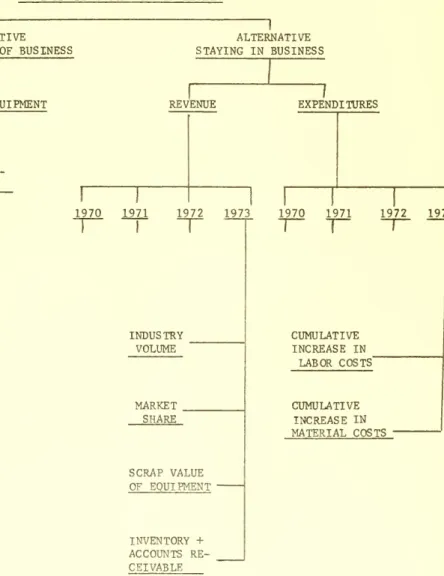
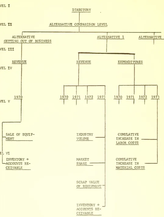
-FIGURE IV

SYSTEM STRUCTURE FOR THE ATHERTON CASE

DIRECTORY

ALTERNATIVE CCMPARISON LEVEL

ALTERNATIVE

GETTING OUT OF BUSINESS

ALTERNATIVE STAYING IN BUSINESS SALE OF EQUIPMENT INVENTORY

+

20

The alternative model for staying in the business is based on

a four-year analysis, four years being the projected life span of

the present equipment. The problem tree or model associated with this

alternative contains four levels. The top level contains one element

which describes the distribution for the total net present value

(after taxes) to the company for staying in the business for the four

year period. It is calculated by taking the discounted after tax

difference between expenditures and revenues for the four years. It

is at this level that the parameters are entered for the price charged

per item for each of the four years and the cost of capital used

by the firm in discounting cash flows. In addition, functional data

are entered for labor cost per item, material cost per item, and

power and supply cost per item, each as a function of the total volume

produced.

The next level contains two elements, one for revenue and another

for expenditures. Revenue is calculated by summing the discounted

revenue cash flows for the four years. Likewise, the total expenditure

element is calculated in the same manner by discounting and summing

the cash flows for expenditures for the four years.

On the revenue side of the problem tree, at the lowest level are

the independent elements for each year for industry volume and market

share. In addition in 1973, which is the last year of the analysis,

elements are provided for subjective estimates for the expected scrap

value of the equipment and the expected return to the company for the

- 21

The revenue generated from product sales for each year is calculated

by multiplying the sales volume for each year by the price charged

for the product. Total volume of sales for the company for each year

is developed by multiplying values independently selected from the

industry volume element and the market share element. A probability

distribution is developed for revenue for each year by repeating this

process a number of times, each time using a different random number

for selecting values from the industry volume elements and the market

share elements.

In the final year of the analysis, in addition to the revenue

generated from product sales, revenue is obtained from selling the

production equipment for scrap and from liquidating the remaining

inventories and accounts receivable. Thus, values are independently

drawn from the probability distributions for scrap value of the

equipment, inventories and accounts receivable, and added to the

sales revenue to yield the total revenue for the year.

On the expenditure side, associated with each year are elements

for describing the subjective probability estimates for expected

cumulative increases in labor costs, and in material costs, expressed

as a percentage increase. All other product cost data are a function

of volume, are known with a high degree of certainty and are specified,

as previously discussed, at the top element of the problem tree. Thus

once a value for the volume of sales for a year is calculated from the

elements on the revenue side of the problem tree, the system uses this

- 22

power, and supplies. The labor and material costs are adjusted by

values obtained from the distributions for the expected cumulative

increase in labor and material costs. Referring to Figure IV,

elements are developed using the independent revenue and expenditures

for each of the four years.

The basic mechanism for forming all of the probability distributions

for the dependent elements is a Monte Carlo process, by means of which

all calculations are iterated through a number of times using a new

set of random numbers for each iteration. One of the problems faced

in the design of the system was to determine how many iterations were

required to insure convergence of the output distributions. To allow

experimentation, a parameter was made available for varying the number

of iterations carried out in developing distributions for the dependent

elements. For the models described here, 100 iterations proved to be

sufficient.

VIII.

SYSTm

The system was designed to allow display of all commands which

are available to the user at any point in the interactive phase of

the analysis. This was done to free the user from having to remember

a long list of commands, and also to eliminate problems caused by

users giving inappropriate commands.

The command options available to the decision maker in the

interactive mode were of two types: (1) movement commands which are

used for moving the system between elements in the model structure, and

- 23

element, such as entering or changing data. A complete description

of the individual commands is given in Appendices I and II.

IX. IMPLEMENTATION

A prototype system was implemented at M.I.T. during the spring

term of 1970 using the Computation Center's CTSS (Compatible

Time-Sharing System). CTSS provided the basic hardware and software needed

to support an interactive visual display device.

The interactive graphical display unit selected was an ARDS

(Advanced Remote Display System) terminal which is a storage tube type

device. The application software for the system were programmed in

the AED language, primarily because of the existence of previously

written software for supporting such visual display devices.

The software development was carried out in two phases. The

first phase, which in turn was subdivided into a number of modules,

was the system supervisor and utility routines to perform system

tasks such as displaying graphs, generating random numbers, etc..

These modules represented the heart of the system and provided the

mechanisms for implementing specific models. Thus this phase provided

the software to support the model-building stage of the

decision-making framework discussed in a previous section.

The second phase of the software development of this prototype

system was the actual implementation of a problem environment. The

environment selected was that of the product decision previously

described. Figure IV shows the problem solution structure implemented.

24

business and a model structure for the alternative for staying in the

business. The second phase consisted of detailing the model structures

in terms of elements, levels, and relationships between the elements

through the use of macro instructions which were developed in the

first phase. In addition, labels and specific command options which

would be made available to the user at each element were specified.

In terms of resources expended for the software development, the

first phase required 350 hours of programming time. This phase is

a "once only" type task in that the software developed can be used for

any problem applications. The second phase, which must be redone for

every new application, required 50 hours of programming time. It is

felt that as more experience is gained with the system, model

implementation programming involved in the second phase can be reduced

to less than 20 hours for most applications.

The operational system conformed to all of the design objectives

specified. One of the most critical variables for insuring the

successful use of the system was gaged to be its response time when

operating in the interactive mode. While response time was a function

of the number of users on CTSS, (CTSS can accomodate up to 30 users)

it never was longer than 15 seconds and normally averaged around

5 seconds.

All user interactions were carried out using the keyboard which

was attached to the terminal. As noted, there are advantages to

using light pen type devices for man-machine interactions. Due to

resource constraints, however, only keyboard interaction was implemented

25

-With regard to the actual computer time used during the

inter-active mode, our initial experience produced a ratio of about 3 minutes

of CPU (Central Processor) time for every hour of terminal time.

The next section will discuss the experiments carried out with

the system to obtain user response data.

X. EXPERIMENT WITH THE SYSTEM

To simulate decision making in an actual business environment

a series of experiments were conducted involving members of the Sloan

School's Senior Executive Program, and Greater Boston Executive

Program as subjects. Most of the participants hold senior management

positions and have had many years of business experience. Due to

time constraints, the experiments concentrated on the last two stages

of the four stage decision-making process discussed, i.e., the Data

introduction and Analysis Stage, and the Decision Stage. That is,

the participants were given a statement describing the problem and

the basic model structures for the possible solutions to the

problem. The problem environment used for all experiments was that

of the product-line decision which was described earlier, in which a

decision was required on whether or not to continue producing a

product. The basic models shown in Figure IV were implemented on the

system. To familiarize the participants with the problem environment,

a case study included in Appendix III and describing the business

situation was given to them. In addition a users*manual (see

Appendix IV) was given to them describing the system and the

26

Twenty-two teams of two members each participated in the experiments

which simulated the last two stages of the four-stage decision-making

process outlined. All experimentation was conducted in an interactive

mode of operation. During the data entering and analysis stage, each

team was required to enter data for both the alternative model for

getting out of the business, and for the alternative model for staying

in the business. Once all data had been entered for a model,

sensitivity analysis could be performed by altering the entered data.

For the model for getting out of the business, data in the form

of cumulative probability distributions were required for the expected

sale price of the equipment and the expected revenues from the

liquida-tion of inventories and accounts receivable. For the alternative

model for staying in the business, data were required for the price

that would be charged for each year of the four-year analysis and the

cost of capital. For each individual year, cumulative probability

distributions were required to specify the company's expected market

share, total industry volume, cumulative percentage increases in

labor costs, and cumulative percentage increases in material costs.

In addition, for the last year of the analysis, cumulative probability

distributions were required for the expected scrap value of the

equipment and the expected revenues from the liquidation of the

re-maining inventories and accounts receivable.

Once all the data which were necessary to completely define a

model were entered, the system computed the cumulative probability

distributions and probability density functions for cash flows for

27

-and net present values after taxes for the model alternative considered.

In order to familiarize the decision makers with the operation of

the system, first, a presentation was given in which the operation of

the system and the model alternatives which were implemented on the

system were discussed. Then each team was allowed to use the system

t

under the guidance of a member of the project group. To save console

time, the individual teams met beforehand to decide on the data they

wished to enter for each alternative model. This phase tended to take,

on the average, two hours. The next phase involved using the system

in the interactive mode for entering data, running models, analyzing

results, and for performing sensitivity analysis. This phase also

averaged two hours, during which data were entered for at least three

alternatives, and sensitivity analysis was performed on each

alternative.

Initial results from the experiments were very encouraging. Most

decision makers were able, after about 15 minutes experience with the

system, to grasp its operation well enough to feel comfortable in using

the commands. They also showed strong indications that they understood

what the system was doing and were not viewing it as a black box. On

the negative side, we found that the executives did not fully adjust to the

use of graphs (distributions of net present values) for comparing

alternatives

.

If we look at the form of the information which the decision maker

could use to discriminate among alternative problem solutions, i.e.,

point estimates for the expected return, estimates of the mean and

28

-graphs of the distributions themselves, the use of the system

influenced the executives to discard reliance on point estimates and

to use the mean and standard deviations as criteria for evaluation

purposes. However, it appears that the user must be exposed to the

system on a number of occasions before he attains the needed expertise

and maturity to appreciate the use of probability distributions in

decision making.

An analysis of the questionnaires completed by all those who

participated in the experiment provided some interesting implications

for decision making systems of this type (a copy of the questionnaire

can be found in Appendix V)

.

1. In attempting to assess the usefulness of a system of this

type we were impressed that the participants strongly indicated that

the system maintained their interest and attention throughout the

sessions. They also tended to underestimate the actual time they

spent on the terminal on the average by a factor of 1/3.

2. In answer to questions related to the individual's like or

dislike for the organization of the system, several important factors

were apparent: (a) As the users became familiar with the models

which were implemented on the system, they tended to come up with

ideas for different model structures. This was in complete agreement

with the hypothesized decision-making framework, in which a decision

maker would, after some experience with working with a set of models,

return to the model formulation stage to alter or develop new models,

(b) For the most part, the users were content with the general command

29

-however, that once an individual had grasped the operation of the

command structure for the system, he would begin to make

recommenda-tions for additional features he felt would be useful. This tended

to verify our hypothesis for the need for system flexibility in

order to individualize the system as the user gains more experience

in its use and applications. Thus the system must have the capability

for (i) acting as a learning device, initially presenting the user

with basic, simple to use, command procedures to allow him to easily

learn the basic capabilities of the system, and (ii) providing the

flexibility needed to satisfy the requests of the user for additional

features as he begins to think of new uses for the system.

Typical responses to the question of "what did you like about

the system" were:

1. It forces the decision maker to structure the problem

and consider all key elements.

2. It provides a methodology for working with risk.

3. It is novel.

4. Its speed allows sensitivity analysis, and consideration

of more possible outcomes, than could be handled in a

manual analysis.

5. It provides graphical presentation of data.

Responses to the question "what did you dislike about the

system" were:

1. Lack of flexibility in structuring the models. As noted,

30

2. Data entering was time consuming. This, of course, is the

drawback of any model in that someone must enter the data.

3. Lack of hard copy. This criticism could be easily overcome

by having a program which would store all results and print

them at some later time on a high speed line printer, or

obtain a hard copy by photographic means.

4. Difficult to keep track of one's position in the problem

tree. This problem can be attacked in two ways. (1)

Pro-vide a "Help" command which would display a figure of the

tree with an arrow pointing to the position presently

occupied by the program. (2) Print out the program's present

position before printing each set of possible commands.

In future versions of IGRAM, one or both of these aids will

be implemented.

XI. CONCLUSIONS

We feel that several important points can be drawn from our

experience with the development and experimentation with a management

decision system based on the coupling of risk analysis models and

interactive visual display devices.

1. We feel that management decision systems of this category

have the potential for being very powerful decision-making tools.

Specifically when used in conjunction with a decision-making framework,

systems of this type provide the decision maker with a methodology

for structuring problems, quantifying risk and establishing criteria

- 31

The process of explicitly stating the decision model in terms

of events and expected outcomes provides a potentially valuable

input to the control and learning process of the organization. As

was discussed in the previous section where we described the

experi-mentation which was carried out, the process of working with models

of alternative courses of action, tends to stimulate the decision

maker to identify other key variables. Thus the system acts as a

learning mechanism.

2. One critical requirement for the successful implementation

of systems of this type is a careful attention to the education process.

The use of subjective probability distributions as an input to models

and the further use of distributions in graphical form as output, is

something which will take the decision maker some time to master.

While the learning period for an individual decision maker will be

partially dependent on his technical background, the more critical

dependency tends to be his willingness to try new ideas.

3. The costs involved in the development and operation of such

systems appear to be well within bounds if general-purpose systems

are designed. By general purpose we mean systems which can be

easily adapted to a new problem environment and a new decision maker.

The system described in this paper was general purpose in that any

model which can be defined in terms of a hierarchical structure whose

elements are defined in terms of probability distributions could be

implemented on the system through the use of macro instructions.

Probably the most valuable contribution the experiment made to

!b>yk>r;;'

-^ca-32

-with little background in management science techniques, can grasp

the concept of the system and make use of it as a decision-making tool

in a relatively short period of time. With regard to the design of

systems of this type, experience with user reactions has indicated

that while an individual decision maker can be trained to become

comfortable with the operation of the system, and thus inferring

that there may not be a need to design a completely new system for

each individual decision maker, the capability must exist for easy

modification of the system. The reason for this requirement lies

in what might be called the "learning effect," which indicates that

as the decision maker becomes more familiar with the system he will

demand that new options be made available to him. The implication

from all this, with regard to a design strategy, may well be that the

initial system should be designed to be very simple for easy master,

but general enough to allow for adaptive growth as the user becomes

more sophisticated in the use of the system.

The experiments carried out with the system have thus far barely

scratched the surface of the potential insights into the man-machine

decision-making process which experimentation with systems of this type

can yield. We feel, however, that the work described in this paper

clearly establishes the feasibility of interactive and graphical

- 33

-APPENDIX I

MOVEMENT CCMMANDS

The three basic command options available for moving around the

problem tree structure are;

1. Move to a higher level. This command is used for upward

vertical movement in the problem tree. This command moves the system

from its present element location to the element in the next higher

level which lies on the branch of the element at which the command

was given.

2. Move to a lower level. This command is used for vertical

movement down the problem tree. After giving this command, a list

is displayed of the elements in the next lower level of the problem

tree. One then can command the system to move to any of the listed

elements.

3. Move to next sequential position. This command is used

for lateral movement in the problem tree along the elements in the

lowest level, i.e., the independent elements. This command sequentially

moves the system along all the lowest level elements of a particular

34

APPENDIX II

FUNCTIONAL CCMIANDS

The functional commands which are available for interaction

with elements are:

1. Re-enter data. This command is used to enter new data or

to alter previously entered data. When at the independent elements,

this command causes the coordinates for the cumulative probability

distribution which are required to specify the distribution to be

displayed. (See Figure V). If for each probability level no value

has been previously entered, the system will pause and wait for the

user to type one in. If a value already exists, it will be displayed.

The user has the option of either typing in a new value or keeping

the old value by typing "new line".

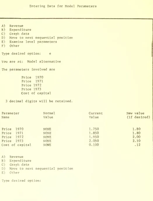
2. Examine level parameters. This command is also a

data-entering command, and is used for entering model parameters, i.e.,

non-probabilistic model values. Figure VI shows an example of this

type of data-entering capability for the price and cost of capital

parameters for a model alternative.

3. Take data from another alternative. This command allows

transferring to an element data which have been previously entered

at another element without having to re-type the data.

4. Graph Data. This command graphs the output of the element

at which the system is located. If one has previously requested the

35

saved graph will also be displayed in addition to the graph for the

element at which the system was located when the command was given.

Figure VII gives an example of the graph of an input distribution,

figure VIII shows a typical model output graph for the distribution

of the expected return after taxes, and figure IX shows the graphs

for functional data for labor costs.

5. Save top, or bottom graph. This command causes the system

to save either the top or bottom graph which is currently being

displayed and to re-display it on the bottom half of the screen the

- 36

-Figure V

Entering Probability Distribution

i^-lf/'-l

- 37

-Figure VI

Entering Data for Model Parameters

A) Revenue

B) Expenditure

C) Graph data

D) Move to next sequential position

E) Examine level parameters

F) Other

Type desired option: e

You are at: Model alternative

The parameters involved are

Price 1970

Price 1971

Price 1972

Price 1973

Cost of capital

3 decimal digits will be retained.

38

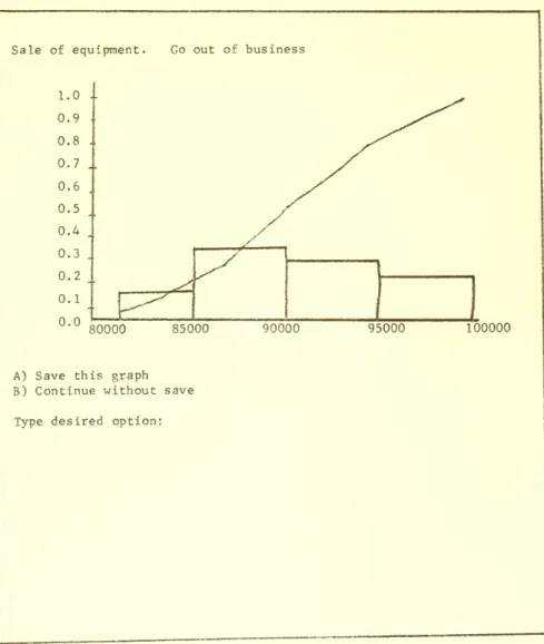
-Figure VII

Graph of distribution entered for the sale of equipment element

Sale of equipment. Go out of business

80000 85000 90000 95000 100000

A) Save this graph

B) Continue without save

- 39

-Figure VIII

Graph of Expected Return from the Alternative of

leaving the business

Go out of business

Mean = 177805. Std. deviation = 5209

1

165000 170000 175000 180000 185000 190000

A) Save this graph

B) Continue without save

40

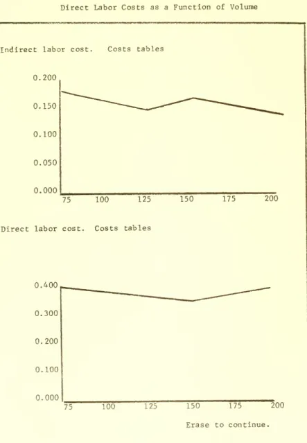
Figure IX

Graphs of Functional Data for Indirect Labor and

Direct Labor Costs as a Function of Volume

Indirect labor cost. Costs tables

0.200 0.150 0.100 0.050 0.000 75 100 125 150 175 200

Direct labor cost. Costs tables

0.400 0.300 0.200 0.100 0.000 75 100 125 150 175 200 Erase to continue.

41

APPENDIX III

ATHERTON COMPANY (A)*

Early in January 1970, the sales manager and controller of the

Atherton Company met for the purpose of preparing a joint pricing

recommendation for Item 345. After the president approved their

recommendation, the price would be announced in letters to retail

customers. In accordance with company and industry practice,

announced prices were adhered to for the year unless radical changes

in market conditions occurred.

The Atherton Company, a textile manufacturer located in Maine,

was the largest company in its segment of the textile industry: its

1969 sales exceeded $6 million. Company salesmen were on a straight

salary basis, and each salesman sold the full line. Most of the

Atherton competitors were small. Usually they waited for the Atherton

Company to announce prices before mailing out their own price lists.

Item 345, an expensive yet competitive fabric, was the sole

product of a department whose facilities could not be utilized on

other items in the product line. In January 1968, the Atherton

Company had raised its price from $1.50 to $2.00 per yard. This

had been done to bring the income contribution per yard on Item 345

more in line with that of other products in the line. Although the

company was in a strong position financially, considerable capital

^Adapted from Anthony, Robert N., Management Accounting: Text and

42

-would be required in the next few years to finance a recently approved

long-term modernization and expansion program. The 1968 pricing decision

had been one of several changes advocated by the directors in an attempt

to strengthen the company's working capital position so as to Insure

that adequate funds would be available for this program.

Competitors of the Atherton Company had held their prices on products

similar to Item 345 at $1.50 during 1968 and 1969. The industry and

Atherton Company volume for Item 345 for the years 1964-1969, as estimated

by the sales manager, are shown in Exhibit I. As shown by this exhibit, the

Atherton Company had lost a significant portion of its former market

position. In the sales manager's opinion, a reasonable forecast of

industry volume for 1970 was 700,000 yards. He was certain that the

company could sell 25 percent of the 1970 industry total if the $1.50 price

was adopted. He feared a further volume decline if the competitive price

were not met. As many consumers were convinced of the superiority of

the Atherton product, the sales manager reasoned that sales of item 345

would probably not fall below 75,000 yards, even at a $2.00 price.

In addition, if the current inflationary pressure remained at its then

present rate, the sales manager believed the general price level across

- 43

-Exhibit I

ATHERTON COMPANY

44

and pre-1960 experience was not applicable due to equipment changes and

increases in labor productivity.

The current inflationary trend, however, had induced a considerable

amount of uncertainty relative tomaterial and labor costs. With regard

to material cost increases, these appeared to be closely correlated with

the general national inflationary rate. On the labor side, while

Atherton was non-unionized, it had adopted a policy of paying competitive

wages.

Exhibit 2

ATHERTON COMPANY

Estimated Cost of Item 345 at Various Volumes of Production (per Yard)

75,000 100,000 125,000 150,000 175,000 200,000

45

-In March of 1970 one of the competitor producers of Item 345 offered

Atherton $90,000 as payment for the equipment used for Product 345. In

view of Atherton's need for funds for modernization and expansion of

other lines, this offer was rather tempting. The Controller pointed

out that a sale of the equipment would not only release the investment

in fixed assets but would also reduce the average inventory and accounts

receivable outstanding by $25,000 and $30,000 respectively. The Controller

felt that a sale would not only produce needed funds but would also

strengthen the company's "quick ratio" when it came time to enter the

market for funds. Furthermore, this was a good opportunity for Atherton

to get out of a losing venture.

The net book value of the equipment now in use for Product 345 was

$160,000 with expected salvage value of $10,000. It was originally

estimated that the economic life would expire at the end of 1974, but

now it appeared that a major rehabilitation would be needed in December 1973

if the equipment were to be used in 1974. Even though no decision was

taken on rehabilitation, Atherton decided not to change its depreciaion

policies but would write off the loss at the end of 1973 in case the

equipment were to be retired at that time.

Atherton was quite a profitable company overall (507, tax bracket),

and only Item 345 was showing losses. Their cut-off return on investment

rate was 107, after taxes, and experience has proven to management's

- 46

Questions

1. Discuss the expected return to the company for various pricing strategies,

(Hint, a time horizon of four years should be used as this is the current

estimated life span of the equipment.)

2. Choose the pricing strategy which you feel offers the company the best

return, taking into account the risks involved.

3, Advise the company as to whether the offer for sale of the equipment

should be accepted or whether the company should stay in the 345 Product

Line, clearly outlining the basis for your decision.

NOTE: A. State any assumptions made, but avoid assumptions that may

define the problem away.

B. Please explain the procedure you used to solve the case

47

APPENDIX IV

IGRAS

interactive Graphical Risk Analysis S^ystem

Introduction

One of the most elusive problems faced by managers today is that

of imposing structure on the decision making process when operating in

an environment in which large amounts of uncertainty exist. Managers

are faced with this problem when they are required to make decisions

concerning such things as capital investments, pricing strategies, new

product development, aquisitions, etc.

When dealing with these types of problems, point estimates of such

variables as market share, industry sales, etc., cannot be taken as

fact, but must be viewed in light of the uncertainty involved in actually

attaining these projections. Thus the manager, in arriving at a decision,

must develop some form of a risk measure for the alternatives under

consideration and perform some types of a trade off between return and

uncertainty. Typically, the decision maker's approach might be to (1) be

overly conservative in estimating return on investment, (2) rely on the

judgement of subordinates who have a good record for making estimates, or

(3) require riskier alternatives to meet higher criteria. Such approaches

have worked in the past and will continue to work in the future, however,

for those decisions which potentially have a large effect on the firm, a

more rigorous approach would seem reasonable. IGRAS presents a possible

approach to the problem of adding structure to problems in which there

are few quantitative data, subjective projections must be made and the

question which is really being asked is, "what is the probability profile

of attaining the projections of the alternative under consideration?"

The basic hypothesis behind IGRAS is that the decision maker, either

- 48

a problem Into basic elements and assign to each of these elements subjective

probability estimates for possible outcomes. For example, in a typical

business decision problem, the basic elements for revenue and expenditure

would be identified. For those elements in which uncertainty is greatest,

further subdivisions could be made until all basic elements of risk have

been identified. Thus the problem would be broken down into a tree like

structure (see Figure 1) with multiple breakdowns along those paths possessing

the most uncertainty.

Figure 1

An Example of the Problem Structuring Process

____Expenditures Net Income _Revenue. -Research ase I Phase II -Production -Marketing Industry Volume .Market Share

49

Once all the majors elements of risk have been identified, and subjective

probability estimates developed for each, the tree structure can be folded

back through combining the subjective probability estimate by means of a

Monte Carlo type process to produce a probability profile of the total

expected return on the investment. The machanism for providing the means

to perform this type of an analysis is an on-line interactive visual display

terminal based system (i.e., a keyboard terminal with a graphical display

tube connected to a computer)

.

Before continuing with the description of IGRAS, four concepts of

probability theory will be reviewed which are critical to the understanding

of the system.

1. Frequency Distribution; A frequency distribution simply portrays

for a given number of trials and a given set of outcomes, how many

times each outcome occurred. Figure 2 gives an example in tabular

form of a frequency distribution for the sales of product 345

for 1970 for 25 trials. In this example, since there are 25 trials,

each occurrence of an outcome represents a 4% probability, i.e.,

25 = 4% 100

Probability Density Function; A probability density function simply

gives the probability that a given level will occur. This can be

developed directly from the frequency distribution realizing that

each outcome represents a 47, probability. Figure 2 shows the density

function which is calculated by multiplying 47, by the number of outcomes

at each level. This function is useful in giving one a feel for the

most likely occurrence (i.e., the mode) and the skewness and variance

50

Figure 2

51

-3. Cumulative Probability Distribution

This function can be derived from the probability density function

and portrays the probability that an outcome will not be exceeded. Figure 3

shows a cumulative probability distribution derived from the previous

example. For example, there is a sales volume of 112,500 units associated

with the 327o probability point on the graph, the meaning being that there

is a 32% probability that actual sales will be 112,500 or less. In

operating with IGRAS you will be required to specify your subjective

estimates in the form of a cumulative distribution. The system will

automatically provide you with the probability density function. In

describing the cumulative probability distribution you will be required

to specify values at the 5%, 10% 25%, 50%, 75%, 90% and 95% probability

levels,

4. Monte Carlo Method of Simulation is a method for operating with

probability distributions. The process is based on the generation of

a random number with values between and 100, with each value having

the same probability of occurrence (i.e., the generation process has a

uniform probability density function). This random number is used to

operate on a cumulative probability distribution by entering the graph

at the probability level equal to the random number (in percent) and

then picking off the value of the function associated with that probability

level. For example, again referring to Figure 3, if the random number

were 32, one would enter the graph at the 32% probability level and pick

off the value for sales of 112,500. This value for sales is used by

the system for all calculations involving sales. A new random number

is then generated and the process is repeated. The results from each

iteration through the process are used to form a frequency distribution,

which in turn could be used to form a new cumulative distribution. Each

time IGRAS runs a model it iterates through the process 25 times, thus

the Monte Carlo Method provides a methodology for combining cumulative

probability distributions. (Note, this concept will become clearer in

Figure 3

52

-Sales Volume Range

37,500 - 62,000 62,500 -87,500 -112,500 -137,500 -162,500 -187,500 -212,500 -87,500 112,500 137,500 162,500 187,500 212,500 237,500 Freque