Determining thermal stratification in rooms under mixing and displacement ventilation

Determining thermal stratification in rooms

mixing and displacement ventilation

by

Francisco Alonso Dominguez Espinosa

JUN

M.S., Mechanical Engineering

_LIB

Massachusetts Institute of Technology, 2011

A

B.S., Mechanical and Electrical Engineering

Instituto Tecnol6gico y de Estudios Superiores de Monterrey, 2008

Submitted to the Department of Mechanical Engineering

in partial fulfillment of the requirements for the degree of

Doctor of Philosophy in Mechanical Engineering

at the

MASSACHUSETTS INSTITUTE OF TECHNOLOGY

June 2016

Massachusetts Institute of Technology 2016. All rights reserved.

aI

A uthor ...

Certified by...S...

Accepted by ...

Signature redacted

...

Depa

_rt...

. . ...

Department of Mechani I Engineering

A9

Febrpary 19, 2016

ignature redacted,

Leon R. Glicksman

Professor of Mechanical Engineering

Thesis Supervisor

Signature redacted

Rohan Abeyaratne

Chair, Committee on Graduate Students

under

isEs INSWUTE

02 2016

RARIES

RCHIVES

Determining thermal stratification in rooms under mixing

and displacement ventilation

by

Francisco Alonso Dominguez Espinosa

Submitted to the Department of Mechanical Engineering on February 19, 2016, in partial fulfillment of the

requirements for the degree of

Doctor of Philosophy in Mechanical Engineering

Abstract

Computational Fluid Dynamics (CFD) simulations of a typical office under both mix-ing and displacement ventilation were performed to study the effects of room geometry (height and area of the supply), ventilation parameters (supply momentum and heat gain intensity) and radiation heat transfer on the thermal stratification of the air and the temperatures of the surfaces in the space. The air stratification and the tem-peratures of the surfaces are two important parameters when determining thermal comfort conditions in the room. Different room configurations were characterized in terms of their Archimedes number, which compares the effects of buoyancy and

sup-ply momentum, and dimensionless geometric variables.

A high Archimedes space was found to be divided into a warm region of uniform

temperature above the occupants and a zone where the temperature increases ap-proximately linearly with height. In a low Archimedes space the air is mixed by the supply jet in the lower part of the room, especially near the outlet, resulting in this area having uniform temperature. However, the supply jet was found to be less effi-cient at mixing the air near the ceiling, resulting in higher temperatures in this zone than with higher Archimedes numbers. For a given Archimedes number, as the

sup-ply area increased, the air temperature was found to decrease in the lower part of

the room but increase near the ceiling. The supply height was found to increase the vertical mixing in the room. Correlations were proposed to establish the temperature profile within 5% of the temperature rise of the room, which include the effects of the Archimedes number and room geometry.

Correlations were developed to estimate the temperatures of the surfaces in a room, based on a dimensionless parameter that characterizes the amount of free area to convect heat to the air. The temperatures of the surfaces were found to be a function of this convective area, regardless of the view factors and convective heat transfer coefficients of the surfaces. A larger amount of convective area was found to result in lower surfaces temperatures but higher air temperatures.

A simple methodology to estimate all of the radiative view factors in an occupied

ignored view factor among occupants can be of importance, not only because occu-pants exchange radiation among themselves, but also because they block radiation that would otherwise reach other surfaces in the room. In addition, techniques to estimate the view factors between other surfaces, such as partitions and furniture, were also developed. Estimated view factors between surfaces encountered in practi-cal situations were found to be within 10% of the results from ray tracing software. The estimated view factors were then incorporated into a thermal resistor network akin to the thermal circuits used to model heat transfer in multizone software. Re-sults from the resistor network showed good agreement with CFD reRe-sults, although the accuracy depends on the convective heat transfer coefficients used. Finally, it was demonstrated that scale models that use water as the working fluid are not capable of replicating the air thermal stratification, the temperatures of the surfaces or the mass flow rate of a full-sized space, because they neglect the effects of thermal radiation transfer.

Thesis Supervisor: Leon R. Glicksman Title: Professor of Mechanical Engineering

Acknowledgments

I thank Professor Glicksman, my PhD adviser, who provided continuous

encour-agement, guidance and advice. I am indebted to Professor Brisson, my adviser during my Master's degree and member of my PhD committee, for all his support throughout my academic life at MIT. Thank you both, Professor Glicksman and Professor Brisson, for believing in me and for giving me the opportunity to work with you. It has been a truly wonderful experience. I also thank Professor Leslie Norford for his valuable advice.

I have learned a great deal from my mates in the Cryogenics Engineering Lab

and in the BT program. Thank you all for your friendliness and support.

Lastly, I would like to thank my family and friends in Mexico for their unwavering support.

This research was funded by the US-China Clean Energy Research Center, the Mexican National Council on Science and Technology (CONACYT) and by the Martin Family Society of Fellows for Sustainability.

Contents

List of Figures List of Tables

Nomenclature

1 Introduction

1.1 Natural ventilation in buildings

1.1.1 Wind-driven ventilation

1.1.2 Buoyancy-driven ventilation 1.2 Modeling natural ventilation . . . . 1.3 Thermal stratification . . . .

1.4 Thermal comfort . . . .

1.5 Literature review . . . .

1.6 Thesis overview . . . .

2 Radiation heat transfer in rooms

2.1 Radiation heat transfer through fluids . . . . 2.2 Previous work . . . .

2.3 M ethodology . . . .

2.4 R esults . . . . 2.4.1 Case A: ceiling 0%; occupants 100% of the total heat gains . . 2.4.2 Case B: ceiling 30%; occupants 70% of the total heat gains and case C: ceiling 50%; occupants 50% . . . .

10 15 17 25 . . . . 2 7 . . . . 2 7 . . . . 2 8 . . . . 3 1 . . . . 3 5 . . . . 3 7 . . . . 4 0 . . . . 4 3 44 46 48 54 59 59 63

2.4.3 Case D: ceiling 100%; occupants 0% of the total heat gains . .

2.5 D iscussion . . . .

2.6 Chapter sum m ary . . . .

3 Improving air thermal stratification model

3.1 Thermal stratification in displacement ventilation . . . .

3.2 Thermal stratification in mixing ventilation . . . . 3.3 Previous thermal stratification model for naturally ventilated rooms .

3.3.1 Description of the CFD model . . . .

3.3.2 Description of the previous thermal stratification model . . . .

3.3.3 Summary of results of previous model . . . .

3.4 Dimensional analysis . . . . 3.4.1 Effect of the Reynolds number . . . .. . . .. 3.4.2 Archimedes and Reynolds numbers in realistic spaces 3.4.3 Effect of some geometrical parameters . . . .

3.5 Effect of the area and height of the inlet . . . .

3.5.1 M ethodology . . . .

3.5.2 Results and discussion . . . .

3.5.3 Modification to previous model . . . .

3.5.4 Comparison to CFD results . . . .

3.6 Chapter summary . . . .

4 Surface temperatures in naturally ventilated spaces

4.1 Heat transfer paths and the effect of the convective area 4.2 M ethodology . . . .

4.3 R esults . . . . 4.3.1 Spaces composed of multiple rows of occupants . . . 4.3.2 Spaces with vertical surfaces: partitions . . . . 4.3.3 Spaces with horizontal surfaces: desks . . . . 4.4 Dimensional analysis . . . . 4.5 Effect of convective area, Archimedes number and inlet area

69 71 76 78 79 84 86 86 88 94 . . . . . 114 . . . . . 120 . . . . . 123 . . . . . 128 . . . . . 133 . . . . . 133 . . . . . 139 . . . . . 152 . . . . . 165 . . . . . 179 181 182 184 189 189 194 194 202 207

4.5.1 M ethodology . . . .

4.6 Results and discussion . . . . 4.7 Chapter summary . . . .

5 View factor estimation in occupied spaces

5.1 Radiation exchange in a room . . . . 5.1.1 Surface properties . . . . 5.1.2 V iew factor . . . .

5.1.3 Geometric representation of a person in a room . . . .

5.2 View factor between occupants . . . ... 5.2.1 View factor between two occupants . . . .

5.2.2 View factor between multiple occupants . . . . 5.2.3 View factor between occupants in wall-bounded rooms . . . 5.3 View factor between occupants and surfaces . . . .

5.3.1 View factors in an infinite space . . . .

5.3.2 View factors in a finite-sized space . . . .

5.4 View factor between surfaces . . . .

5.4.1 Infinite room . . . . 5.4.2 View factors in spaces with vertical surfaces: partitions . . . 5.5 C onclusions . . . .

6 Resistor network model

6.1 Description of the model . . . .

6.2 Convective heat transfer coefficient in ventilated rooms

6.3 M ethodology . . . .

6.4 Results and discussion . . . . 6.4.1 Heat transfer coefficients . . . . 6.4.2 Temperatures of the surfaces . . . .

6.5 Chapter summary . . . .. . . . 275 . . . . . 276 . . . . . 281 . . . . . 287 . . . . . 288 . . . . . 288 . . . . . 294 . . . . . 298 207 208 215 217 218 218 219 223 227 227 231 240 245 245 248 257 257 259 273

7 CoolVent 300

7.1 Model ... ... 301

7.1.1 Airflow network . . . . 301

7.1.2 Energy conservation equation . . . 304

7.1.3 Coupling schemes . . . 305

7.1.4 Thermal stratification . . . 306

7.2 Description of the interface of CoolVent . . . 307

7.2.1 Main inputs . . . . 307

7.2.2 Transient inputs . . . 309

7.2.3 Building and openings geometry . . . 309

7.2.4 Ventilation strategies . . . . 310

7.2.5 Thermal comfort model . . . 312

7.2.6 R esults . . . . 312

7.3 Chapter summary . . . . 313

8 Conclusions and future work 315 8.1 Conclusions . . . . 315

8.2 Future work . . . . 320

List of Figures

1.1 Example wind-driven ventilation . . . . 29

1.2 Examples buoyancy-driven ventilation . . . . 30

1.3 Examples wind catchers . . . . 31

1.4 Filling box . . . . 33

1.5 Adaptive comfort standard . . . . 38

1.6 Graphic comfort zone method . . . . 40

2.1 Absorption coefficient and penetration depth of water . . . . 47

2.2 Stratification profiles in water, R144 and air from [76] . . . . 51

2.3 Thermal stratification profiles from [62] . . . . 52

2.4 Geometry of the CFD model . . . . 53

2.5 Symmetry and adiabatic planes . . . . 55

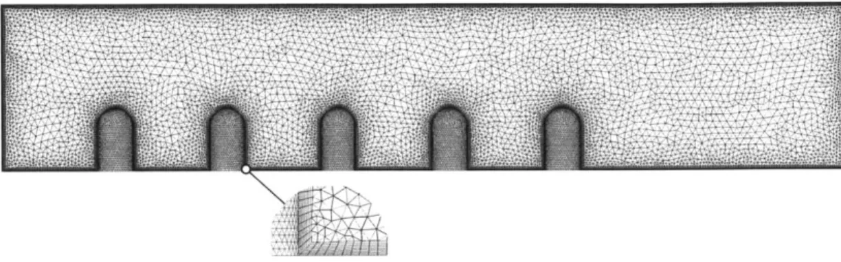
2.6 M esh . . . . 57

2.7 Measurement planes . . . . 59

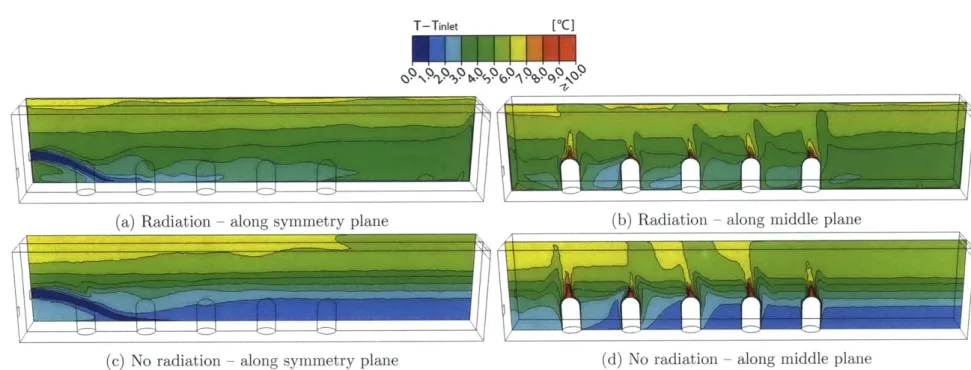
2.8 Case A temperature contours . . . . 60

2.9 Case A planes temperatures . . . . 61

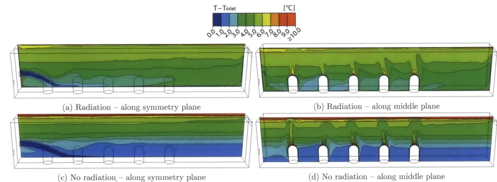
2.10 Case B temperature contours . . . . 64

2.11 Case C temperature contours . . . . 65

2.12 Cases B and C planes temperatures . . . . 66

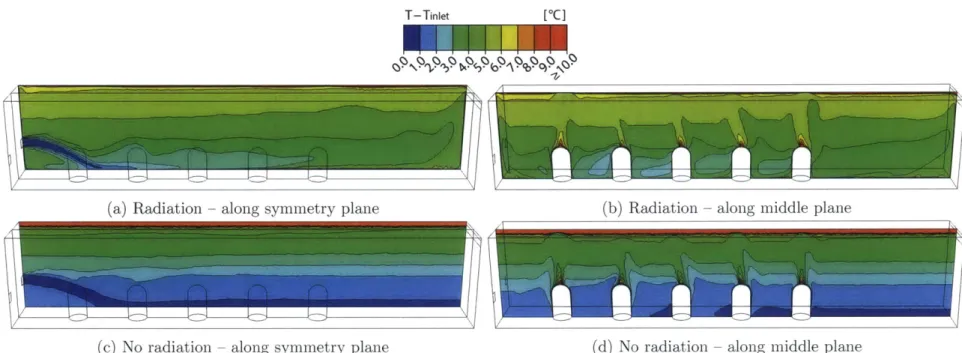
2.13 Case D temperature contours . . . . 70

2.14 Case D planes temperatures . . . . 72

2.15 Case D outlet detail . . . . 72

3.1 Four-node profiles . . . . 81

3.2 Resistor network of the model by Mundt . . . . 82

3.3 Space geom etry . . . . 86

3.4 Measurement planes . . . . 89

3.5 Simplified temperature profiles . . . . 90

3.6 Comparison CFD and existing stratification models . . . . 93

3.7 Effect of inlet velocity . . . . 96

3.8 Effect of inlet height . . . . 100

3.9 Effect of inlet area - temperature contours . . . . 103

3.10 Effect of inlet area . . . . 104

3.11 Effect of inlet area - velocity contours . . . . 106

3.12 Effect of inlet area - occupant plume streamlines . . . . 107

3.13 Effect of heat gains - temperature contours . . . . 110

3.14 Effect of heat gains . . . 111

3.15 Comparison original, 5 times inlet area . . . . 113

3.16 Example dimensional analysis . . . . 118

3.17 Effect of the Reynolds number . . . . 124

3.18 Deviation due to Reynolds number . . . . 125

3.19 Realistic Archimedes and Reynolds numbers . . . . 127

3.20 Room with two occupants per row . . . . 128

3.21 Effect of number of occupants . . . . 131

3.22 Effect of number of occupants - temperature contours . . . . 132

3.23 Deviation due to occupants . . . . 133

3.24 Effect of number of Archimedes number - temperature contours . . . 140

3.25 Effect of Archimedes number . . . . 142

3.26 Effect of Archimedes number on stratification profile . . . . 143

3.27 Effect of the inlet area - temperature contours . . . . 145

3.28 Effect of the inlet area - temperature contours . . . . 146

3.29 Effect of the inlet area . . . . 147

3.31 Effect of the inlet height - temperature contours

3.32 Effect of the inlet height

3.33 AOacf against Arh, .

3.34 AOacf against Arha .

3.35 Oac against Arh . . . . ..

3.36 Height of the interface 3.37 AOac5o against Arh, ..

3.38 AOac5o against Arh, .

3.39 Comparison to CFD . . . 3.40 Comparison to CFD . . . 3.41 Comparison to CFD . . . 3.42 Comparison to CFD . 3.43 Comparison to CFD . 3.44 Comparison to CFD . . .

4.1 Heat paths in room . . . . 4.2 Model of naturally ventilated office . . . . 4.3 Space with two rows of occupants . . . . 4.4 Vertical surfaces: separations . . . . 4.5 Horizontal surfaces: desks . . . .

4.6 Effect of room width - surface temperatures . . .

4.7 Effect of number of room width - air temperature 4.8 Deviation due to room width . . . .

4.9 Partitions - surface temperatures . . . . 4.10 Partitions - surface temperatures . . . . 4.11 Deviation due to separations . . . . 4.12 Desks - surface temperatures . . . . 4.13 Desks - air temperature . . . . 4.14 Deviation due to desks . . . . 4.15 Surfaces dimensionless temperatures . . . . . . . . . . . . . . . . . . . . . . . . - . . . . ... ---. ...-- . . . . . . . . 182 184 185 186 187 191 192 193 195 196 197 199 200 201 206 . . . . 150 . . . . 151 . . . . 154 . . . . 155 . . . . 158 . . . . 161 - . . . . . 163 . . . . 164 . . . . 167 . . . . 169 . . . . 171 . . . . 173 . . . . 175 . . . . 177

4.16 4.17 4.18 4.19 5.1 5.2 5.3 5.4 5.5 5.6 5.7 5.8 5.9 5.10 5.11 5.12 5.13 5.14 5.15 5.16 5.17 5.18 5.19 5.20 5.21 5.22 5.23 5.24 5.25 210 211 214 215

Surface temperatures against A* and Arhw . . . . . .

Surface temperatures against A* and Arh . . . .

Of,, against #C . . . .

0_{f,w against 6c, different inlet areas . . . .}

Fanger's view factors . . . . Representation of a person . . . . Test geom etries . . . . Surfaces in right cylinder and rounded-top cylinder . . View factor between two finite cylinders . . . . Occupant grid . . . . Shadow ing . . . . Partial shadowing . . . . Crossed-strings method . . . . View factor between occupants in infinitely wide and lo E rror . . . . Subdivided grid . . . . View factors from occupants in infinite room . . . . Shadowing to surfaces due to occupants . . . . Shadowing to surfaces due to occupants . . . . Method to estimate shadowing . . . . Shadowing to surfaces due to occupants . . . . View factors from ceiling in infinite room . . . . View factors in infinite room with separations . . . . . View factor from ceiling to partitions . . . . View factor from ceiling to partitions . . . .

F₀,Np against 1,* H*, N . . . ..

View factor from ceiling to wall in room with partitions View factor from wall in room with partitions . . . . . View factor from wall to ceiling in room with partitions

. . . . 222 . . . . 224 . . . . 225 . . . . 228 . . . . 229 . . . . 232 . . . . 233 . . . . 234 . . . . 236 ng room . . . 239 . . . . 239 . . . . 241 . . . . 248 . . . . 249 . . . . 251 . . . . 253 . . . . 255 . . . . 258 . . . . 259 . . . . 261 . . . . 265 . . . . 266 . . . . 268 . . . 269 . . . . 271

Heat paths in room . . . . Heat paths in room - well mixed . . . . Comparison of convective heat transfer coefficient calculated using CFD and correlations . . . . Surface temperatures against A* - resistor network . . . . Surface temperatures against A* - resistor network . . . . Surface temperatures against A* - resistor network . . . .

6.1 6.2 6.3 6.4 6.5 6.6 7.1 7.2 7.3 7.4 7.5 7.6 7.7 276 278 293 295 297 299 . . . . 306 . . . . 308 . . . . 308 . . . . 310 . . . . 311 . . . . 312 . . . . 314 CoolVent algorithm . . . .

CoolVent Man Inputs tab . . . . Other building geometries . . . . CoolVent Transient Inputs tab . . . . CoolVent flow elements specification . .

CoolVent Thermal Comfort Models tab . Results from CoolVent . . . .

List of Tables

2.1 Lighting and occupant heat gain division . . . . 56

2.2 Excess temperatures of the floor and the ceiling for cases B and C . . 67 3.1 Dimensional values of the parameters used in the simulations of Figure

3 .7 . . . . 9 5

3.2 Dimensional values of the parameters used in the simulations of Figure

3.8 ... ... .. . ... ... 98

3.3 Temperature of the ceiling and floor for different inlet heights . . . . 99

3.4 Dimensional values of the parameters used in the simulations of Figures

3.9 and 3.10 . . . . 102

3.5 Dimensional values of the parameters used in the simulations of Figure

3 .13 . . . . 109

3.6 Relevant variables in the thermal stratification problem . . . . 114

3.7 Dimensional values of the parameters used in the simulations of Figure

3 .17 . . . . 122

3.8 Dimensional values of the parameters used in the simulations of Figure

3 .2 1 . . . . 129

3.9 Parameters used in CFD simulations . . . . 135

3.10 Parameters used in CFD simulations by Menchaca Brandan [61] . . . . 137

3.11 Expressions to calculate the fitting parameters of Equation 3.22 . . . 156

3.12 Range of validity of the expressions of the fitting parameters of Table 3.11 .... ... ... ... ... .. .. ... . .. ... 156

3.13 Expressions to calculate the temperature of the air near the ceiling,

Oac, and their range of validity . . . . 159

3.14 Expressions to calculate the fitting parameters of Equation 3.23 . . . 162 3.15 Range of validity of the expressions of the fitting parameters of Table

3 .14 . . . 165

4.1 Values of the parameters used to analyze the effect of the Archimedes number, inlet area and convective area . . . . 208

4.2 Archimedes and Reynolds numbers used in the CFD simulations . . . . 208

4.3 Values of the fitting constants in Equation 4.7 . . . 212 4.4 Values of the fitting constants in Equation 4.8 . . . 213 4.5 Values of the fitting constants in Equation 4.9 . . . . 213 5.1 View factors from an occupant to the surrounding surfaces in a room 226

5.2 View factors between surfaces S1+S₃ of two right cylinders for different

separations between them . . . 230

5.3 View factors from the occupants to the different surfaces in a room . 256

5.4 View factors from the occupants to the different surfaces in a room with separations . . . . 260 6.1 Selected correlations to estimate the convective heat transfer coefficient 286

6.2 Convective heat transfer coefficients used to generate Figure 6.4, taken from CFD simulations . . . 294

6.3 Convective heat transfer coefficients used to generate Figure 6.5 ob-tained from correlations . . . 296

Nomenclature

Greek symbols

a thermal diffusivity

#3

A change in variable

6P penetration depth

APrise pressure rise across fan

AOac5O difference in dimensionless temperature of air near ceiling and at half the

height of room

AOacf difference in dimensionless temperature of air near ceiling and near floor

AOacf difference between dimensionless air temperature near ceiling and near floor

ATr air temperature rise across room

rlfan fan efficiency

A wavelength, spectral

A dynamic viscosity

vI kinematic viscosity

<5 correction factor

p density

a- Stefan-Boltzmann constant

7-W shear stress at a wall

0 dimensionless temperature, angle between infinitesimal surface normal and line connecting to second infinitesimal surface

Oac dimensionless air temperature near ceiling

Oac dimensionless air temperature near ceiling

OC average dimensionless ceiling temperature

Of average dimensionless floor temperature

OW average dimensionless walls temperature

0_{surface average dimensionless temperature of surface}

Oa dimensionless air temperature

Roman symbols

A incidence matrix

A area, fitting constant

Aac5 0 fitting constant

Ac ceiling area

ACH air changes per hour

A*e dimensionless free convective area

Af floor area

a fitting constant Ar Archimedes number Aw inlet area

A* dimensionless inlet area

B fitting constant

Bac5 0 fitting constant

C fitting constant

c column index, constant

Cd discharge coefficient

CP wind pressure coefficient

CP specific heat capacity at constant pressure

cV specific heat capacity at constant volume

D fitting constant

DH hydraulic diameter

Dmax maximum deviation

E emissive power matrix

E fitting constant

e error

erms root-mean-square error

F emissivity and view factor matrix

f

Fijj view factor from surface i to surface

j

Fmax fitting constant

g acceleration of gravity

H room height

h height

he,f convective heat transfer coefficient between floor and air near floor

hinterf interface height in a two-layer temperature profile

herf dimensionless interface height in a two-layer temperature profile

ho height of occupants

he convective heat transfer coefficient

hr radiative heat transfer coefficient

hr,cf linearized radiative heat transfer coefficient between ceiling and floor

h* dimensionless height

hw inlet height

h* dimensionless inlet height

I intensity

J radiosity matrix K Laplacian matrix

K constant

kij element (i,

j)

L room length, characteristic length

1 thickness of thermal mass

f characteristic length of surface

1* dimensionless length rn mass flow rate

M number of surfaces

N number of surfaces that form an enclosure n number of resistances connected to node

Ns number of separations Nu Nusselt number

P pressure

PW perimeter of surface Pr Prandtl number

Q

Q

R radius vector between two occupants, thermal resistance

r radius of occupant

Ro radius of auxiliary cylinder Ra Rayleigh number

Rcf convection resistance between floor and air near floor Re Reynolds number

R1 ,f radiation resistance between ceiling and floor

S length of line connecting two infinitesimal surfaces T temperature matrix

T temperature

t time

Ta air temperature

Taf temperature of the air near the floor

T average temperature

Th temperature at head level Tiniet inlet temperature

Tm mean temperature, temperature of layer m of thermal mass Toutiet outlet temperature

Tsurface average temperature of surface

TWM well-mixed temperature

U vector

U fraction of uncovered area

u inlet velocity

f a average air speed in room

V volumetric flow rate

V volume

v wind speed

W room width

W* dimensionless room width

X distance between cylinders/occupants

x x coordinate

y distance from wall, y coordinate

y + dimensionless distance from a wall

Z height from the floor

z z coordinate

Subscripts

a air air air

c ceiling, convection cold cold wall

f

h, c heating and cooling hot hot wall

i index

00 outdoor

1-j

max min

TMass thermal mass

w window, inlet

Superscripts

complete occupant fully surrounded by other occupants corner occupant at corner of room

* dimensionless quantity

u unblocked

occupant next to a wall index maximum minimum nearest-neighbor approximation operative opening

occupants and equipment convection

room, mean radiant, radiation

0 0 o, e C r wall

Chapter 1

Introduction

According to the United States (US) Energy Information Administration [1], in 2015 commercial buildings represented approximately 20% of the total energy consumed in this country. Fifteen percent of the energy consumed by commercial buildings is used for cooling and ventilation. This energy consumption has annually released more than 1,000 million metric tons of CO2 since 2000. Both the energy load and

associated greenhouse emissions can be considerably reduced by using passive cooling technologies in buildings. Natural ventilation has become one of the most common cooling technologies in new commercial buildings [91]. When properly designed and implemented, natural ventilation can maintain comfortable thermal conditions and good indoor air quality in a space. Additionally, natural ventilation mitigates many of the problems of mechanical cooling systems, including high capital and maintenance costs, and health problems such as the "sick building syndrome" [81]. Thanks to its many advantages, natural ventilation is not only preferred by occupants over air conditioning, but has also been suggested as a factor leading to increased employee productivity [58, 81]. Although commonly used in domestic buildings and in the developing world, it only recently has been re-introduced in the US, Europe and Japan as an effective way to ventilate commercial buildings.

To properly design and manage a naturally ventilated building it is necessary to evaluate the thermal and airflow conditions in it. Models used to assess the

comfort conditions in a space depend on several factors, with the temperature of the air near the occupants and the temperatures of the surfaces surrounding them (e.g. ceiling, walls, floor, furniture, etc.) as two of the most important ones [3]. Therefore, a knowledge of the temperature distribution in the space is critical to ensure that natural ventilation can meet the comfort requirements of the occupants. Due to the high velocities and, as a consequence, the high level of air mixing in natural ventilation, it is common to assume that the temperature of the space is uniform and equal to the exhaust temperature. Unfortunately, this assumption has been shown to substantially overestimate the temperature of the air near the occupants, and thus underestimate the potential of natural ventilation to meet comfort conditions [61]. For this reason, natural ventilation is underused, and potential energy savings and associated reduction of greenhouse gases are not realized.

To overcome the problems related to the assumption of uniform temperature, several researchers (refer to the literature review, Section 1.5) have used scale models in experimental work and/or simple theoretical models to try to predict the thermal stratification profile of the air as well as the temperatures of the surfaces in a space. Scale models that use water of different salinities to represent air at different temperatures have been used to study the thermal stratification in naturally ventilated rooms (e.g. [44, 56, 85]). However, water models have been shown to be unable to reproduce the stratification seen in real spaces, due to the stark difference in radiation transport properties of water and air [62, 76]. Traditionally, theoretical stratification models have been developed under the assumption that the velocity of the air supplied to the room is low enough as to ignore the effect of its momentum on the air temperature profile. However, this assumption is not always valid in naturally ventilated spaces. Only recently have new models been developed that include the effect of the momentum of the supply air [61]. Unfortunately, these models do not properly account for all the main pa-rameters that have an effect on the air thermal stratification, as is shown in this work.

Although significant progress has been achieved in the last few years, more work is still necessary to improve the prediction of the temperature distribution in a room. Hence, this thesis improves an existing model to increase the accuracy of the predicted temperature profile of the air in the room and establishes a new method to compute the temperature of the surfaces in the space. As part of the calcula-tion of the surface temperatures, a novel methodology to quickly and accurately approximate the view factors between the surfaces and the occupants of the space was also developed. The models presented in this thesis are simple enough to be used during the early stages of the design process of a new building. These models have been incorporated into CoolVent, a computer design program for naturally ventilated spaces, so they can be used easily when analyzing the performance of natural ventilation in buildings. Additionally, the influence of radiation heat transfer on the temperature distribution and airflow rate in a space was also studied. This study shows that ignoring radiation exchange, as effectively done when using water in scale models, results in inaccurate predictions of not only temperature profiles, but also of airflow rates. In general, the results presented in this thesis illuminate the effect of radiation, room geometry, furniture, occupancy heat gains and the supply air momentum on the thermal and airflow dynamics in a naturally ventilated space.

1.1

Natural ventilation in buildings

1.1.1

Wind-driven ventilation

The easiest way to use natural ventilation is to open the windows in a space. With the right outdoor conditions, a pressure difference between multiple openings is developed, and this pressure difference, in turn, drives the flow of air in the space. The magnitude of the pressure difference depends on the position and geometry of the openings, the geometry of the space and the outdoor wind conditions [10, 31]. The pressure difference generated by the wind can be obtained from experimental data or computer

simulations. These data have been compiled for different building geometries and are expressed in terms of the wind pressure coefficient, Cp, defined as follows:

P

C =p2 (1.1)

where P is the pressure (with respect to some reference pressure), po is the density of outdoor air, and vo is the wind speed far from the influence of the building [31]. The value of C, is larger for a wall facing windward and smaller for the wall facing leeward [10]. The difference in pressure between two openings, AP, is given in terms of the difference between the wind pressure coefficients associated with each opening,

1 2

AP = pOv 2ACP (1.2)

In pure wind-driven ventilation, the flow rate of air through the space is independent of the heat gains in the space.

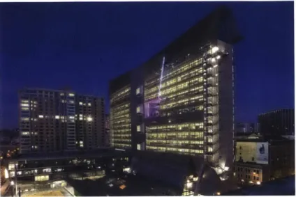
The San Francisco Federal Building in California, shown in Figure 1.1, is an example of a building that was designed to use wind-driven ventilation [8]. The San Francisco Federal Building is a thin building, with the smallest dimension in the same orientation as the principal wind direction to reduce the pressure drop across the building, thereby increasing the wind-driven flow of air [8].

1.1.2

Buoyancy-driven ventilation

Buoyancy-driven ventilation refers to the flow of air caused by differences in the density of the air. The difference in densities is a consequence of the difference in air temperature in different zones. For a single room at a uniform temperature with two identical openings at different heights, the pressure difference between these two openings is given by:

Figure 1.1: The San Francisco Federal Building was designed to take advantage of wilnd-driven ventilation. Image from [8].

where Ap is the difference between the air density outside the space, usually ambient. density, pj, and inside, pi, g is the acceleration of gravity, and 1 is the height difference between the two openings. Atria and ventilation shafts take advantage of buoyancy forces by increasing the height difference between the air inlet(s) and outlet(s) to increase the flow rate of air in a building [81]. Solar chimneys use solar heat gains to increase the temperature difference, and thus the density difference, between the outdoor air and the air in the chimney to achieve higher airflow rates [811.

In buoyancy-driven ventilation, the heat gains in the space directly influence the amount. of air flowing into the space by changing the temperature, and thus the density, of the air in the space. At, the same time, the air that is drawn into the interior changes the temperature of the space. Therefore, the governing equations of flow and energy balance that describe buoyancy-driven ventilation are coupled [31]. These coupled equations can be solved analytically only for the simplest cases, so an iterative scheme is needed for buildings with multiple connected spaces. Realistic combined buoyancy-, wind- and mechanical-driven ventilation cases cannot be solved analytically given the coupling of the flow and thermal equations.

(a) (b)

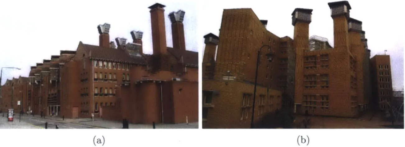
Figure 1.2: (a) The Queen's Building of the De Montfort University (image from

[16]), and (b) the Frederick Lanchester Library of the Coventry University (image from [68]) take advantage of the stack effect to increase the airflow rate of

buoyancy-driven ventilation.

Figure 1.2 shows the Queen's Building of the De Montfort University [27] and the Frederick Lanchester Library of the Coventry University [74], both in the United Kingdom. These buildings use ventilation towers to enhance buoyancy-driven

ventilation.

"Wind catchers" look similar to exhaust, ventilation shafts, but instead of driving the air from the interior, they direct cold air from the exterior to the warmer interior. Evaporative cooling is needed to decrease the temperature of the air entering the wind catcher to below the anbient temperature, so that it flows downwards along the chimney of the wind catcher [13]. Figure 1.3a shows wind catchers in the city of Yazd, Iran. Wind catchers are a, traditional element of Persian vernacular architecture found also in other Middle Eastern countries [13]. Figure 1.3b shows the building of the Global Ecology Research Center of the Carnegie Institution of Science at, Stanford University [75]. The tower in this building is a wind catcher.

(a) (b)

Figure 1.3: (a) Wind catchers in traditional Persian architecture (image from [24]).

(b) A wind catcher is used to ventilate the Global Ecology Research Center at

Stanford University (image from [75]). The second floor of this building is fully naturally ventilated using a combination of wind and buoyant forces.

1.2

Modeling natural ventilation

Natural ventilation is a simple concept, but its application has not been without challenges. Designing a successful naturally ventilated building is not trivial, in part due to the difficulty of accurately modeling the airflow dynamics in a space. Among the challenges the designer of a naturally ventilated space faces are: (i) natural ventilation depends on weather conditions that are subject to sudden and generally unpredictable changes, (ii) wind-, buoyancy- and mechanical-driven ventilation are not independent, but act in a coupled way, and (tIu) rooms are rarely isolated, depending instead on the conditions of other connected rooms [31].

Designers have access to several tools to analyze natural ventilation in buildings, including Computational Fluid Dynamics (CFD) software., scale models and mnultizone nodal networks [19]. CFD simulations provide detailed information regarding the air-flow pattern and temperature field iii a room. Moreover, CFD can be used in transient studies of the thermal mass of the building and its interaction with the air flowing in the space. Nevertheless, CFD is time consuming, computationally expensive and

requires a high degree of expertise to set up correctly, especially for large buildings with multiple connected spaces. For these reasons, these simulations are impractical to study the performance of the building under many different weather conditions or to compare different designs of a building. Instead, they are more suitable for the final stage of the design process, when the geometry of the building is well defined.

Another method used to study natural ventilation in general, and buoyancy-driven flows in particular, is with scale models. Dynamic similarity between the scale model and the full-sized space is required for the results of the model to be representative of the real space. Dynamic similarity can be achieved by matching the Reynolds number and the Grashof or the Archimedes number, a dimensionless number that captures the effect of the buoyant forces, as well as inertial forces, for both the model and the real space [79]. Nevertheless, scale models that use air as the working fluid are not practical, because similarity generally requires using very high temperatures in the model [79]. Instead, water of different salinities, and therefore of different densities, has been-and is still-used, due to its many advantages over air, including simple visualization of the flow pattern, straightforward measurement of density profiles using conductivity probes, and more importantly, the possibility of attaining dynamic similarity under realistic conditions [56]. Figure 1.4 shows a picture of a "filling box" used to study the airflow in a building under buoyancy-driven ventilation.

Unfortunately, previous research has shown that scale models that use water do not reproduce the actual flow pattern nor the temperature stratification of the air in a real building [62]. The work by Menchaca-Brandan and Glicksman [62], as well as earlier work by Olson et al. [76], demonstrated that the reason for this discrepancy is the difference in the behavior of water and air regarding radiation heat transfer. While water is generally opaque to infrared radiation, even for very thin water layers, air is practically transparent to radiation exchange in spaces with moderate humidity [54]. Radiation exchange thermally connects the ceiling, floor, walls and other surfaces in the room, so the temperature difference between these

Figure 1.4: A filling box uses water of different salinities to represent air of different temperatures in a scale model. Image from [43].

surfaces is significantly lower than when radiation is not available to transfer heat. As a consequence, with available exchange through radiation, the temperature of the air is higher at the occupant zone but lower near the ceiling, and the two-layer temperature profile, with its abrupt change in temperature, seen in Figure 1.4, is replaced by a continuous temperature profile that changes uniformly from floor to ceiling. Additional research that complements the results by Menchaca-Brandan and Glicksman regarding the effect of radiation on the niass flow rate through a room is presented in Chapter 2 of this thesis. All these studies demonstrate that using scale models with water results in inaccurate predictions of nattural ventilation in rooms.

Multizone airflow networks divide the building into different zones of uniform tem-perature. This simplification is known as the "well-mixed assumption". These zones are represented as pressure nodes in a resistor network. The resistances connecting these nodes characterize the pressure drops due to viscosity as well as flow restrictions and obstructions. For windows, air vents and doors, the static pressure difference be-tween two nodes and the resulting airflow rate bebe-tween then are related by a power

law known as the "orifice equation", given by:

Zijj= sgn (A Pi,) CdA 2 ' (1.4)

p2

where VIy is the volumetric flow rate from zone i to zone j through the opening that connects them, Cd and A are the discharge coefficient and area, respectively, of the opening, AP,1 is the static pressure difference across the orifice, p2 is the density of

the air through the opening, and sgn is the sign function [31]. The pressure difference across the opening is given by:

APj,j = ( Pi - P ) - g [ pi (h,, - hi ) - pj (h, - hj)] + sgn (v.) _PO.V P (1.5)

where P and P are the reference pressures at heights hi and hj from the ground for zones i and j, respectively. pi and p3 are the density of zone i and j, respectively, h, is

the elevation of the opening with respect to the ground. voc, and pc are the free wind velocity and the outdoor air density, respectively, Cp is the wind pressure coefficient, which is equal to zero for interior sides of the openings. sgn (vO) is positive if the free ambient wind flows from zone i to zone j, and vice versa. The air density depends on the amount of heat gains in the zone and the temperature of the air entering the zone.

The solution of the multizone network consists in finding the values of the static pressures of the nodes that satisfy the mass and energy conservation equations simul-taneously for each zone. These equations are, respectively:

Vi dt r~j. - ri (1.6)

dTd

PViCv,air d = o,e + Qh,c + QTMass +

Z

where V, and T are the volume and temperature in zone i, Cv,air is the heat capacity at constant volume of air, o,e is the occupant and equipment heat load, Qh,c is the

net heat gain due to mechanical heating (positive) and cooling (negative), QTMass is the heat transfer from the thermal mass of the building, rmj,i and mhij are the mass flow rate into and from zone i from/to j, cp,ajr is the heat capacity at constant pressure of air, and T is the temperature of zone j. Solar heat gains are first absorbed

by the thermal mass, before being transferred to the air via convection heat exchange.

Multizone networks are faster and easier to use than CFD simulations, although they do not provide as much detail as CFD. The well-mixed assumption is an impor-tant shortcoming of the multizone model, as it leads to an inaccurate assessment of comfort conditions in the room. One of the goals of this thesis is to improve the model used to estimate the thermal stratification of a room to overcome this shortcoming.

1.3

Thermal stratification

In the well-mixed assumption, the temperature of the air in a room is presumed to be constant and equal to the exhaust temperature. In an actual room, although the air near the exhaust is indeed close to the well-mixed temperature, near the inlet the temperature is colder. Furthermore, due to buoyant forces, the temper-ature of the air near the ceiling is warmer than the air near the floor, so the occupants of a room are generally located in a zone where the air is colder than the well-mixed temperature. As a consequence, room models that rely exclusively on the well-mixed temperature underestimate the potential of natural ventilation to keep the occupants under comfortable conditions. Additional problems arising from using the well-mixed assumption have been identified, including an inaccurate estimation of the air mass flow rate in a space under buoyancy-driven ventilation [51].

Given that the airflow and thermal comfort conditions in a room depend on the temperature stratification of the space, a model that can be used to incorporate

thermal stratification in a multizone network is desirable. Such a model needs to be fast to test multiple building designs and under different weather conditions. To build this kind of model, substantial experimental and theoretical work has been produced, including the work by Hunt and Linden [45], Li [50] and Mundt [65], among others (refer to the "Literature review" section for more details). The vast majority of this work has dealt only with conditions of negligible momentum of the air supplied to the room (known as displacement ventilation), although recent research has looked at the situation for which this momentum is not negligible (mixing ventilation). Nielsen

[69] proposed using the Archimedes number, the ratio of buoyancy forcescaused by

the heat gains in the room and the inertia of the colder jet coming in through the inlet, to predict the thermal stratification of the room. However, this research was only qualitative. The Archimedes number is defined as follows:

gO3ATrhw

Arh, = 2 (1.8)

where g is the acceleration of gravity, 0 is the volumetric thermal expansion coefficient of air, AT, is the air temperature change across the room (i.e. ATr = Toutiet - Tiniet), h, is the height of the inlet and u is the inlet velocity [69].

A simple and fast model to quantitatively predict the thermal stratification in

a space, based on two forms of the Archimedes number, has been presented in the work by Menchaca Brandan [61]. The model is based on two alternative forms of the

Archimedes number: gOATrh3 Arh,= u2_Aw (1.9) g3ATr (H - hw)3 _(1.10) Arh,,' u2_Aw

where A, is the inlet area, and H is the height of the room. Fitting results obtained from CFD simulations, Menchaca Brandan presented correlations to approximately predict the thermal stratification of a space [61]. However, the CFD simulations of this author did not explore the effect of different inlet heights and areas. Chapter

3 of this work builds upon the results by Menchaca Brandan by investigating the

effect of different inlet areas and heights.

1.4

Thermal comfort

Thermal comfort is the collection of physical, physiological and psychological con-ditions under which a person expresses satisfaction regarding his/her environment. Because thermal comfort is subjective, different people, even with comparable levels of activity and clothing, can choose different environmental conditions under which they feel comfortable [3]. Moreover, experimental work has shown that just the availability of control over the thermal conditions in a space can shift the response of an occupant regarding being comfortable or not [26].

During the last 90 years, models have been developed to evaluate thermal comfort of a person in a given environment. Simple models depend on a combi-nation of environmental indices that determine the comfort levels of test subjects. Other models, including the work by Fanger [32], calculate the heat exchange of a human with his/her environment, and relate this heat exchange with perceptions of comfort/discomfort. Thermal comfort can be assessed by bands of conditions under which a certain percentage of people would be comfortable, or by the level of satisfaction/dissatisfaction with the environment [3].

For naturally ventilated buildings, the ASHRAE Standard 55-2010 includes an optional method to determine acceptable thermal conditions, called the "adaptive standard". This standard is valid for a space that has no air conditioning, although it could have mechanical ventilation in the form of, for example, ceiling fans. Nevertheless, the primary means of regulating the temperature of the space must be by opening and closing windows. Users must have access to such controllable windows and should be free to change their clothing, i.e. they should be able to

34 32 -30 28' *._ 26 E a) 24 -S22 Qj 90% acceptability 2 20- 80% acceptability-0 0 18 16 14' 10 15 20 25 30 35

Mean monthly outdoor air temperature [0C]

Figure 1.5: Graphical representation of the adaptive comfort standard [3]

adapt to-and be able to adapt-their local environment [3].

Graphically, the adaptive comfort standard is shown in Figure 1.5. There are two regions in this figure, delineating the conditions for which 80% and 90% of the occupants in a space would feel comfortable. The parameters defining comfort in this case are the monthly average outdoor temperature and the indoor operative temperature. The mean monthly outdoor temperat-ure is tlie arithmetic average of the mean daily mininmnu and mean daily maximum dry-bulb outdoor temperature. The operative temperature. To, is a weighted average of the mean radiant, temperature,

T, and the air temperature surrounding the occupants, T, with the weighting factors

being the radiation, h, and convection, h, heat transfer coefficients:

hrTr + heTa

To =h ~(1.11)

It, + h,

Physically, the operative temperatunre can be interpreted as the temperature of an-other body or surface with which the occupant exchanges the same amount of heat as in the space. Such exchange of heat happens with an effective heat, transfer coefficient

equal to h, + h,. The mean radiant temperature is the temperature of a blackbody enclosure, which would exchange the same amount of radiative heat with the occu-pants as the actual space they occupy. The mean radiant temperature is a function of the view factors between the occupant and the surfaces surrounding said occupant [3].

It is a remarkable feature of the adaptive comfort standard that it does not depend on humidity in any manner, nor does it depend on the air speed that the occupants experience, as long as it is below a maximum velocity threshold. Another important feature of this standard is the fact that it depends on solar radiation only through the operative temperature, but not on whether the occupant is directly under the solar rays [3].

Thermal comfort conditions in a space with hybrid natural-mechanical ventilation can be evaluated using the adaptive comfort standard explained above, only if no air conditioning is available. For ventilation systems that do include air conditioning, a different standard must be used. The ASHRAE 55 thermal comfort standard in this case takes the form of an area on a psychometric chart with operative temperature in the x axis, delineating the conditions under which the occupants would feel comfortable, as shown in Figure 1.6. In this case, comfort depends not only on the operative temperature, but also on the humidity of the space and the clothing of the occupants. Also, there are limits to the air speed in this standard, which depend on the specifics of the method used to assess thermal comfort [3]. This method is generally referred as the "graphic comfort zone" method, a somewhat confusing name given that the adaptive comfort standard is also presented as comfort zones in a graph.

The operative temperature is an input in both the adaptive and the graphical comfort standards. To compute the operative temperature, the temperature of the air near the occupants, as well as the mean radiant temperature for the occupants, needs to be calculated. However, current multizone tools are incapable of computing any of these temperatures accurately. Moreover, other sources of discomfort, such

25 20 15 10 1.0 0.5E 0) 400/0 20% 0 15 20 25 30 35 Operative temperature ['C]

Figure 1.6: The graphic comfort zone method of the ASHRAE 55-2010 thermal comfort, standard. Two zones are shown, representing areas under comfort

conditions for different clothing levels [3].

as a large air temperature difference between the head and the feet of the occupant, cannot be assessed using models that rely on the well-mixed assumption. This thesis presents simple models to calculate air and surface tenperatures to better evaluate the thermal comfort conditions in a space than was previously possible.

1.5

Literature review

The thermal stratification profile of a room has been the subject. of substantial research, both experimentally and theoretically. Several researchers have determined experimentally the temperature profile of rooms, particularly under mechanical ventilation (e.g. [15]). This experimental work has shown that the temperature profile in the room is not always linear with height, a common assumption in some theoretical work [20, 73]. Instead, the experiments demonstrated the existence of two regions in the room, a lower zone of cold air and a warm zone above it. In this regard, Nieniela and Koskela [73] reported a warm layer of almost uniform temperature in the upper zone of an industrial workshop. Based on experimental results, qualitative

relations between conditions in the space (ventilation rate, heat source type and position, etc.) and its thermal stratification have been developed by Li et al. [53], Nielsen [70, 73], and Sandberg and Blomqvist [80], among others. However, no guidance was presented to estimate quantitatively the thermal stratification of a space.

Analytical solutions are generally based on assumed temperature profile shapes. Therefore, the objective of the analytical models is only to determine the value of the temperature at some locations along the profile. Commonly, these locations are the temperature near and/or at the ceiling, and near and/or at the floor. Linden et al. [56] presented a model, based on their experiments with filling boxes (e.g. Figure 1.4), that divides the room in two zones of uniform temperature: a lower region at the supply temperature and an upper warm zone at the exhaust temperature. In this model, no heat transfer (radiation or convection) occurred between the ceiling, the floor and the air. Li [50] extended this model to account for the heat transferred between these surfaces and the air by allowing the temperature of the ceiling and the floor to be above that of the air surrounding them. Besides the profile by Linden et al., Li also proposed a second temperature profile that is linear from the air near the ceiling to the air near the floor. Because the conditions of a space that would lead to one profile or the other were not given, this model is of limited practical use. Furthermore, all these models assumed a single heat source in a room of a rather simple geometry.

Mundt [65] proposed a simple analytical method to estimate the temperature profile under displacement ventilation, based on the flow of heat in a room. In this model, the temperature of the ceiling is assumed to be identical to the temperature of the air at the exhaust, because the outlet of a displacement ventilation system is located at, or near, the ceiling level. The ceiling is a warm surface facing down, so convection is an inefficient heat transfer mechanism. Thus, most of the heat transfer from the ceiling occurs via radiation to the floor. The heat is then convected

to the air near the floor. This amount of heat is also responsible for raising the temperature of the supply air to the temperature of the air near the floor. Finally, the temperature profile is assumed to be linear from the temperature of the air near the floor to the ceiling. Good agreement between the model and experimental results was found. However, Mundt only compared the value of the difference in the temperature between the air near the ceiling and near the floor, but did not assess the actual shape of the stratification profile.

Chen and Glicksman [20] developed a semi-empirical model to predict the thermal stratification of the air in displacement ventilation that focused particularly on the temperature gradient between the head and the feet of the occupants, because this gradient is useful in evaluating comfort in the room. The authors simulated typical geometries of small and large offices, classrooms and workshops using a CFD code, so that the results are relevant to realistic spaces with more than a single occupant. From these simulations, they extracted fitting coefficients to determine the temperature difference between the head and the feet of the occupants, accounting for both different ventilation rates and multiple types of heat sources. In this model, the temperature is assumed to change linearly from the zone near the floor to the head, although no shape is given for the temperature profile from the head to the ceiling or from the floor to the zone near the floor.

More recently, the interaction of the wind- and buoyancy-driven components of natural ventilation has been investigated. Hunt and Linden continued working with the simple model of two layers at uniform temperature with no heat transfer, including the effect of wind when it assists [45] and when it opposes [43] the buoyancy forces. Menchaca Brandan [61] proposed a model based on multiple CFD simulations of a typical naturally ventilated office to predict the thermal stratification profile of the room, showing that the well-mixed assumption results in an overestimation of the temperature at the occupant height in most cases. Nevertheless, this model is still incomplete, as it does not predict the temperature of the surfaces in a room.