PEOPLE'S DEMOCRATIC REPUBLIC OF ALGERIA MINISTRY OF HIGHER EDUCATION AND SCIENTIFIC RESEARCH
FERHAT ABBAS SETIF-1 UNIVERSITY
FACULTY OF TECHNOLOGY
THESIS
submitted to the Electronics Department
To obtain a diploma of
DOCTOR IN SCIENCES
By
REFOUFI Salim
THEME
Control of autonomous mobile robot by quantitative inference
Defended the 23/12/2018 with the committee members:
CHEMALI Hemimi Professor Univ. F. Abbas Setif 1 President
BENMAHAMMED Khier Professor Univ. F. Abbas Setif 1 supervisor
BERTIL Arres Professor Univ. F. Abbas Setif 1 examiner
ABDESSEMED Foudil Professor Univ. Hadj Lakhdar Batna examiner BOUMEHRAZ Mohamed Professor Univ. M.Khieder Biskra examiner TAIBI Mahmoud Professor Univ. Badji Mokhtar Annaba examiner
Thanks
Praise to ALLAH the Almighty, the All Merciful and the Most Merciful, to have given us the patience, willingness and the necessary force to realize this project.
I expressed my profound thanks to mythesis director Prof. K Benmahammed for the responsibility ensuring and for encouraging and supporting me in our project, I also express my sincere gratitude for the trust who testified to me throughout this work.
I extend my sincere thanks to the jury members, Mr.CHEMALI Hemimi Professor at the University of F. Abbas SETIF-1 for accepting preside this work, Mr. BERTIL Arres Professor at the University of F. Abbas SETIF-1, Mr.ABDESSEMED Foudil Professor at the University of Hadj. Lakhdar Batna, Mr.BOUMEHRAZ Mohamed Professor at the University of M.Khieder Biskra,
Mr.TAIBI Mahmoud Professor at the University of BadjiMokhtar Annaba,for agreeing to judge this work.
I wanted to thanks greatly
• The staff of the electronics department.
iii
Summary
Summary
GENERAL
INTRODUCTION ... 1
1.1. State of the art ... 1
1.2. Problem studied ... 2
1.3. Theproposed approach ... 3
1.4. Thesis organization ... 3
Chapter 01 ... 3
MODELING AND CONTROL OF ROBOTS
... 3
1.1. Introduction... 3
1.2. Manipulator robots ... 3
1.2.1. Dynamic model...3
1.2.1.1. Lagrange Formalism ...3
1.2.1.2. Model of the robot with two degrees of freedom (d.o.f) ...4
1.3. Trajectory generation ... 5
1.4. Control techniques of manipulator robots ... 5
1.4.1. Classic control...5
1.4.2. Improving the tracking by the control ...7
1.4.2.1. Non-linear decoupling control...7
1.4.3. Predictive dynamic control ...9
1.4.4. Adaptive control ... 10
1.4.4.1. Different adaptive controls ... 10
1.4.4.2. Approaches for manipulator arm analysis... 12
1.5. Mobile robots ... 14
1.5.1. Definition of a mobile robot ... 14
1.5.2. Wheeled mobile robots ... 14
1.5.3. Classification of wheeled mobile robots ... 15
1.5.3.1. Classification according to the type of wheels ... 15
iv
1.5.4.1. Wheel model ... 15
1.5.4.2. Modeling hypothesis ... 15
1.5.4.3. Rolling without slip and non-holonomy ... 16
1.5.4.4. Kinematic model of unicycle wheel robots (differential) ... 17
1.5.5. Dynamic model of unicycle wheeled robots ... 18
1.6. Properties and Control of a mobile robot ... 19
1.6.1. Definitions,PropertiesandLinearization... 19
1.6.1.1. Frobenius Theorem [35] ... 22
1.6.1.2. Feedback Linearization [37] ... 23
1.6.1.3. Input-state Linearization [37] ... 25
1.6.1.4. Input-Output Linearization [37] ... 26
1.6.1.5. Feedback Linearization (Internal dynamics) [37] ... 27
1.6.1.6. Controllability about a Trajectory... 28
1.6.1.7. Static Feedback Linearizability (Chained Forms) [38]... 30
1.6.2. Trajectory Tracking ... 31
1.6.2.1. Feedforward Control Generation... 31
1.6.2.2. Linear Control Design ... 31
1.6.2.3. Nonlinear Control Design ... 32
1.6.2.4. Dynamic Feedback Linearization ... 33
1.7. Conclusion ... 35
Chapter 02 ... 36
T
HEG
ENETIC ALGORITHMS(GA
S). ... 36
2.1. Introduction... 36
2.2. Genetic algorithms ... 36
2.2.1. history ... 36
2.2.2. Definition of a GAs ... 37
2.2.3. Operating principle of GAs ... 37
2.3. Fitness Technique ... 39
2.3.1. Direct transformation ... 39
2.3.2. Windowing ... 40
2.3.3. Linear scale change... 40
2.4. Operating mechanism of a GAs ... 41
v
2.4.2. Coding and decoding of parameters... 42
2.4.2.1. Coding ... 42 2.4.2.2. decoding ... 43 2.4.3. Genetic operators... 43 2.4.3.1. The selection ... 43 2.4.3.2. Reproduction ... 45 2.5. Convergence ... 49 2.6. Advantage of GAs ... 50 2.7. Limitation of GAs ... 50 2.8. Conclusion: ... 50
Chapter 03 ... 51
F
UZZY LOGIC,
N
EURAL NETWORKS,
N
EURO-
FUZZY... 51
3.1. Introduction... 51
3.2. Fuzzy logic principle ... 51
3.2.1. Fuzzy sets ... 52
3.2.1.1. Fuzzy subset ... 52
3.2.2. Linguistic variable ... 54
3.2.3. Fuzzy characterization ... 54
3.2.4. Proposals and fuzzy rule ... 54
3.2.4.1. Activation of a fuzzy rule... 55
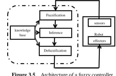
3.2.5. Classic architecture of a fuzzy controller (FLC) ... 55
3.2.5.1. Fuzzification ... 55
3.2.5.2. Inference: ... 56
3.2.5.3. Defuzzification ... 58
3.3. Neural networks ... 59
3.3.1. Definition of a biological neuron ... 59
3.3.2. The artificial neuron: ... 60
3.3.3. Function of the neuron ... 60
3.3.4. Formal neuron ... 61
3.3.4.1. Model of Mc Culloch and Pitts [47] ... 61
3.3.5. Some models of ANNs ... 62
3.3.5.1. Multilayer ANNs ... 62
vi
3.3.5.3. CMAC-type ANN [49] ... 68
3.3.6. ANN training by Kalman Filter ... 69
3.4. Fuzzy logic and neural networks ... 70
3.4.1. Multi-layered neuro-fuzzy networks... 71
3.4.1.1. Coding of fuzzy subsets ... 72
3.4.1.2. Calculation of the degree of activation of the premises ... 72
3.4.1.3. Inference and defuzzification ... 73
3.4.1.4. Examples of the multilayer network ... 74
3.5. Conclusion ... 78
Chapter 04 ... 79
R
ESULTSAND DISCUSSIONS... 79
4.1. Introduction... 79
4.2. The first application ... 79
4.2.1. Trajectory generation ... 80
4.2.2. Application of the fuzzy control ... 80
4.2.2.1. Fuzzy controller with three membership functions ... 80
4.2.2.2. Fuzzy controller with five membership functions ... 83
4.2.2.3. Fuzzy controller with eleven membership functions ... 84
4.2.2.4. Comparative analysis ... 85
4.2.2.5. Justification ... 86
4.2.3. Neuro-Fuzzy Regulator (2×2) ... 86
4.2.4. Control Algorithm ... 87
4.2.5. Training Algorithm ... 87
4.2.6. Neuro-fuzzy control optimized by GAs ... 88
4.2.7. Simulation results ... 89
4.2.8. Practical results ... 95
4.3. Second application ... 97
4.3.1. Kinematics modeling ... 97
4.3.2. The trajectory tracking control ... 98
4.3.3. Linear Control Design ... 99
4.3.4. Nonlinear Control Design ... 100
4.3.5. Dynamic Feedback Linearization ... 100
vii
4.3.7. Simulation results ... 101
4.3.8. Practical results ... 104
4.4. Conclusion ... 107
viii
List of Figures
Figure 1.1 Representation of the robot with two rotational axes...4
Figure 1.2 Generation of an interpolation polynomial. ...5
Figure 1.3 Classic diagram of a PID control. ...6
Figure 1.4 Diagram of a dynamic control by nonlinear decoupling. ...8
Figure 1.5 Predictive dynamic control. ... 10
Figure 1.6 Block diagram of the gain-scheduling control. ... 11
Figure 1.7 Synoptic diagram of an adaptive reference model system. ... 11
Figure 1.8 Block diagram of a self-adaptive regulator. ... 12
Figure 1.9 Error model ... 13
Figure 1.10 Illustration of Lyapunov's method ... 14
Figure 1.11 Diagram of the different wheels types of the mobile platforms ... 15
Figure 1.12 Description of a wheel ... 16
Figure 1.13 UnicycleRobot type ... 17
Figure 1.14 Fluid control in a tank ... 24
Figure 2.1 Flowchart of the GAs. ... 38
Figure 2.2 Relationship between ability and cost. ... 40
Figure 2.3 Fitness function, a) direct transformation,b) windowing, c) linear change of scale. ... 41
Figure 2.4 The five levels of organization Figure 2.5 Schematic illustration of the ... 42
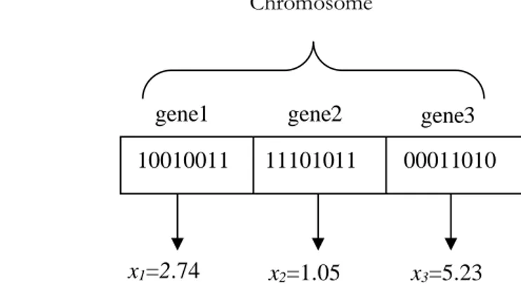
Figure 2.6 Each gene (each parameter of the device) is encoded by a long integer (32 bits). ... 43
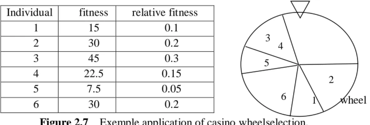
Figure 2.7 Exemple application of casino wheelselection. ... 44
Figure 2.8 Application of the « stochastic remainder without replacement selection » to theprevious example. ... 44
Figure 2.9 One-point crossover. ... 46
Figure 2.10 Two-point intersection. ... 46
Figure 2.11 Uniform crossover. ... 47
Figure 2.12 Mutation. ... 49
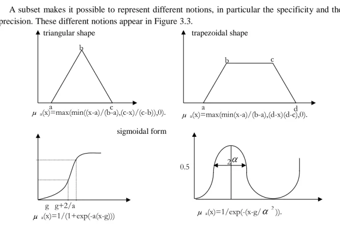
Figure 3.1 Example of sets definition on a universe of discourse in binary logic and fuzzy logic. ... 51
Figure 3.2 Support, kernel, and height of a trapezoidal function. ... 52
Figure 3.3 Form of membership functions... 53
Figure 3.4 Representation of a linguistic variable defined as
V,U,TV
A1, A2, A3, A4
... 54Figure 3.5 Architecture of a fuzzy controller. ... 55
Figure 3.6 Continuous fuzzification with three membership functions. ... 56
ix
Figure 3.8 Defuzzification by the method of the maximum. ... 59
Figure 3.9 A neuron with its dendritic arborization ... 60
Figure 3.10 Mapping biological neuron to artificial neuron. ... 60
Figure 3.11 Different types of threshold functions for the artificial neuron... 61
Figure 3.12 General models of neurons. ... 61
Figure 3.13 A multilayer network with 2 input neurons, 4 hidden neurons ... 62
Figure 3.14 Activation function of a hidden neuron with a single input. ... 66
Figure 3.15 Discretization of a two-dimensional input space by a CMAC-type network. ... 68
Figure 3.16 Local generalization property of a CMAC network. ... 69
Figure 3.17 Kalman filter phases ... 70
Figure 3.18 An example of a neuro-fuzzy network architecture. ... 71
Figure 3.19 Minimum (x, y) and softmin (x, y) functions. ... 73
Figure 3.20 Approximation of the function Maximum (0, x) (dashed) by a sigmoid (in a continuous line). 73 Figure 3.21 Defuzzification by local average maxima. The fuzzy subset corresponding to the result of the rule is shown in gray... 74
Figure 3.22 Fuzzy rule system in the form of a NAN (Mamdani). ... 75
Figure 3.23 System of fuzzy rules in the form of an NAN (Sugeno). ... 77
Figure 4.1 The ROBAI Cyton arm. ... 79
Figure 4.2 Membership functions, FLC of three membership functions. ... 81
Figure 4.3 Response of the system.(Fuzzy- regulatorof 3 membership functions). ... 81
Figure 4.4 Response of the system.(Fuzzy- regulatorof 3 membership functions). A. letting load of 0.18 Kg, B. letting load of 0.36 Kg. ... 82
Figure 4.5 Response of the system.(Fuzzy- regulatorof 3 membership functions). Rupture drive. ... 82
Figure 4.6 Membership functions, FLC of 5 membership functions. ... 83
Figure 4.7 Response of the system.(Fuzzy- regulatorof 5 membership functions). A. without load.B.with load... 83
Figure 4.8 Response of the system.(Fuzzy- regulatorof 5 membership functions). ... 84
Figure 4.9 Membership functions, FLC of 11membership functions. ... 84
Figure 4.10 Response of the system.(Fuzzy- regulatorof 11 membership functions). A. without load.B.with load... 85
Figure 4.11 Response of the system.(Fuzzy- regulatorof 11 membership functions). ... 85
Figure 4.12 Regulator of the Sugeno (2×2) type in the form of ANN. ... 86
Figure 4.13 Neuro-Fuzzy Subsets Form-Genetic Control algorithm (N-FSF-GC). ... 88
Figure 4.14 The trajectory of the two joints. ... 92 Figure 4.15 Response of the system for a tracking,without load. A. Neuro-fuzzy regulator of the
x
Sugenotype, C. Neuro-fuzzy-genetic regulator of (2×2) Sugenotype with three interpolation points,
where the point in the middle optimized by GAs. ... 93
Figure 4.16 The membership functions for the two regulators (e : error, ∆e : error variation), A. Before optimization, B. After optimization of the sub-set fuzzy (normalization gains of fuzzification), C. After three interpolation points, where the point in the middle optimized by GAs. ... 93
Figure 4.17 Response of the system.( Neuro-fuzzy-genetic regulator of (2×2) Sugenotype), after five interpolation point. A. without load.B.with load. ... 94
Figure 4.18 The membership functions for the two regulators (e : error, ∆e : errorvariation) after five interpolation points, where the three points inside the curve optimized by GAs. ... 94
Figure 4.19 Response of the system.( Neuro-fuzzy-genetic regulator of (2×2) Sugenotype), after five interpolation points with fall of load from 0.36 Kg to 0 Kg at 3.6 sec time. A. one keeps the same membership functions of 0.36 Kg. B. one changes the membership functions from 0.36 Kg to 0 kg at 3.6 sec time... 95
Figure 4.20 Same practical results as in figure 4.15. ... 96
Figure 4.21 Same practical results as in figure 4.17. ... 96
Figure 4.22 Same practical results as in figure 4.19. ... 97
Figure 4.23 Kinematic representation of a mobile robot unicycle type. ... 98
Figure 4.24 The trajectory tracking control of the mobile robot. ... 99
Figure 4.25 The Eight-shaped reference trajectory. ... 101
Figure 4.26 Trajectory tracking. ... 101
Figure 4.27 Trajectory tracking, LCD.Linear Control Design, NCD.Nonlinear Control Design. ... 102
Figure 4.28 Trajectory tracking, PD-DFL.Dynamic feedback linearization, NF-DFL.Neuro-fuzzy Dynamic feedback linearization before optimization. ... 102
Figure 4.29 Trajectory tracking, PD-DFL.Dynamic feedback linearization, NF-DFL.Neuro-fuzzy Dynamic feedback linearization after optimization. ... 103
Figure 4.30 Trajectory tracking with initial error, PD-DFL.Dynamic feedback linearization, NF-DFL.Neuro-fuzzy Dynamic feedback linearization after optimization. ... 103
Figure 4.31 Cartesien motion (x, y) (m) with an initial error. ... 104
Figure 4.32 The mobile robot PioneerP3-DX ... 105
Figure 4.33 Same practical results asin figure 4.27. ... 105
Figure 4.34 Similar practical results as in figure 4.29. ... 106
Figure 4.35 Similar practical results as in figure 4.30. ... 106
xi
List of tables
Table 3.1 Inference matrix... 57
Table 4.1 Rules base ... 80
Table 4.2 Basic rules, FLC (5 × 5). ... 83
Table 4.3 Basic rules, FLC (11 × 11). ... 84
Table 4.4 The tracking errors at the end of trajectory of the two joints. ... 86
Table 4.5 Parameters of ROBAI Cyton. ... 91
Table 4.6 Parameters of GAs. ... 91
Acronymes
d.o.f ANN
Degree of freedom
Artificial neural networks
FNNs Fuzzy neural networks
FLS Fuzzy Logic System
GAs Genetic algorithms
PID Proportional/integral/derivate MFs Membership functions E-L Euler-Lagrange D-H Denavit-Hartenberg w.r.t With respect to s.t Such that
LTI Linear time invariant
LHP Left-half plane
e.s Exponentially stable
DFL Dynamic Feedback Linearization
Symboles M(q) : H(𝑞, 𝑞̇): G(q) : F(𝑞, 𝑞̇): m1: m2 : mp G1 : G2 : L1 : L2 : Lc1 : Lc2 : m : I : d : r : R: l, r: : q : 𝑞̇ : 𝑞̈ : τ : Inertia matrix. Coriolis/centrifugal vector. Gravity vector. Friction torque Body mass 1. Body mass 2. Load mass.
Center of body mass 1. Center of body mass 2. Body length 1.
Body length 2.
Center of mass position G1 compared to O1. Center of mass position G2 compared to O2. The mobile robot mass.
The moment of inertia of the robot about its center of mass.
The distance between the center of mass and the center of the wheel axle. The wheel radius.
Half distance between the two wheels. The motor torques on the wheels. The constraint force.
Vector joint positions. Vector joint velocities. Vector joint accelerations.
1
GENERAL
INTRODUCTION
1.1. State of the art
Faced with the delicate problems of modeling and control of the complex systems such as the robots, the tools used are becoming increasingly cheaper and more powerful. The PID has proven its effectiveness in many problems of the industrial regulation. However, if the precision is required, it becomes inapplicable because of its linearity. In the recent decades, many research works have shown that the nonlinearities generate specific phenomena and these had to be taken into account to study the system in a satisfactory manner. Indeed, either these phenomena are undesirable, and then the knowledge of their mechanisms is essential to avoid them, or it is inevitable and intrinsic to the system itself, then it must be understood and modeled, or it must beintroducedfor the purpose of well-defined applications. Therefore, one needs the introduction of other algorithms to develop new powerful controllers [1,2]. An approach having experienced significant developments these last years is the fuzzy controller relating to the systems containing knowledge: “IF (conditions) THEN (Action)" [3]. In spite of the significant number of applications developed by the fuzzy control, it always lacks tools that make it possible to analyze these controllers [4,5]. To avoid the problem of the expertise, the researchers tried to replace the expert by several methods such as the neural networks and the genetic algorithms.
Neural networks are based on the mechanisms of operations of the human brain, in the form of layers [6,7,8]. The genetic algorithms are also very much used for the optimization of fuzzy regulators. They are based on the theory of evaluation of the most adapted elements of a generation towards the other, so that the best adapted ones would last in time, while the other should disappear. The proposed adaptive neuro-fuzzy optimized by GAscontrol scheme has some advantages over classical fuzzy control and neural networks control schemes [9,10]. For example, in a classical fuzzy controller design, some controller parameters must be tuned by trial and error. Such parameters include scalars (or gains) for its inputs and outputs data, the number of membership functions, the width of a single membership function, and the number of control rules [11,12,13,14,15,16,17,18,19,20,21]. On the contrary, the adaptive neuro-fuzzy controller based on the dynamic model estimation would allow the parameters to be tuned automatically [22]. In addition, the performance of the neuro-fuzzy controller optimized by GAs is also considered to be excellent.
The neuro-fuzzy-genetic controller does not require knowledge of the robot parameter values. It needs, neither system dynamic model nor control experts for the robot control problem.
The application of neuro-fuzzy to the manipulator robot has motivated considerable research in this area in recent years. In [23], an adaptive control using multiple incremental fuzzy neural networks (FNNs) was presented. The controller is combined by a feedback controller and several
FNNs to learn inverse dynamics of the manipulator robot for different tasks. The several FNNs
are obtained dynamically using an incremental hyper-plane-based fuzzy clustering algorithm to compensate the unknown disturbances of the system. In [24], a decentralized intelligent control method for a robust control of underwater manipulator was developed. The controller is based on
2
a neuro-fuzzy approach where the feedback gains are adapted using fuzzy logic, whereas a neural network is used to add to the controller a feed-forward compensation input. The neural network is trained using the back-propagation approach to estimate the system dynamics from the input-output data. Therefore, the proposed method does not depend on modeling and dynamics estimation system. The same authors in [25] proposed an intelligent controller used a neuro-fuzzy approach for precise control, robust and energy efficient. The decentralized controller is a PD type, with fuzzy setting feedback gains modified using modified fuzzy membership functions. The magnitude of the gains and thus, the energy expenditure is reduced by the neural network based on the identification of the system dynamics and hydrodynamic disturbances. In [26], a comparative study of several hybrid neuro-fuzzy adaptive control systems to control the six degrees of freedom (Puma 560) robot arm, with uncertainties were presented. The proposed controller combines ANFIS based controllers, with some well established traditional controllers (computed torque control, feed forward inverse dynamics, and critical damping inverse dynamics control).
In [11], both orthogonalization and passivity properties are taken into account to design a neuro-fuzzy system (NFS) like a PID controller to ensure tracking by exploring a new energy re-shaping of the closed loop system through a self-optimization of the dissipation rate gain (DRG) without any knowledge of the robot dynamics. In [12], Fuzzy Logic System (FLS) was presented to generate the rules using neuro-fuzzy methods. In [27], a single hidden layer in a fuzzy recurrent wavelet neural network (SLFRWNN) was developed and used for the function approximation and the identification of dynamic systems. And in [28], a supervised training algorithm based on sliding mode theory that implements fuzzy reasoning on a spiking neural networks, for the trajectory control problem of a robotic manipulator was developed and tested. In [29], a new neuro-fuzzy classifier which draws its inspirations from the concepts of the linguistic hedges was used.
1.2. Problem studied
For a manipulator robot which carried loads, control planning becomes a problem even more difficult to solve than in the case where the robot contains parameters poorly modeled. The robot is subjected to new constraints generated by its contact interaction with the environment, and can not be neglected in a drive generation process. In this work we used a neuro-fuzzy-genetic controller to drive the robots. The neural networks are proposed for the automatic extraction of the fuzzy rules, using a Kalman filter as a training means. To optimize the location of the fuzzy subsets, the GAs are used, and since there are several forms of the fuzzy subsets such as triangular, Gaussian…, the choice of the appropriate form becomes a problem. Thus the variation of the load carried by the robot causes the dynamics of the manipulator to lose the tracking.
For the mobile robot from a control viewpoint, the peculiar nature of nonholonomic kinematics makes that feedback control at a given trajectory cannot be achieved via smooth time-invariant control. This indicates that the problem is really nonlinear, linear control is ineffective, even locally, and innovative design techniques are needed.
3 1.3. Theproposed approach
The work presented in this thesis is describes the displacementscontrol of a robot carrying a load. To well learn dynamics of the manipulator robot, which represent an extension of the idea given by [25] and [29] where they used a triangular membership functions (MFs), with linguistic hedges to modify the shape of the MFs. In this work, we used a neuro-fuzzy-genetic controller. The neural networks are proposed for the automatic extraction of the fuzzy rules, using a Kalman filter as a training means. To optimize the location of the fuzzy subsets, we used the GAs, and since there are several forms of fuzzy subsets such as triangular, Gaussian, etc…, and as a contribution, we used an interpolation function with three points, and then with five points, for each fuzzy subset, and we optimized the curves by the GAs, to find the most suitable shape of a fuzzy subset, which is going to be adapted according to the load. The same idea applied for the control of a mobile robot using dynamic feedback linearization as linear control and we replace the PD compensator by a Neuro-fuzzy-Genetic controller.
1.4. Thesis organization
This thesis proposes a hybrid type controller that combines a fuzzy regulator adapted by neural networks, and optimized by genetic algorithms.
It is organized as follows:
The first chapter is devoted to a geometric, kinematic and dynamic modeling of a robot arm, and a mobile robot of differential speed, as well as the generation of trajectories, and their control techniques.
The second chapter treats the general description of the genetic algorithms functioning.
The third chapter presents the theoretical basis of fuzzy logic, generalities on neural networks, and a combination of the two to obtain a neuro-fuzzy controller.
In the fourth chapter, we presente the different fuzzy control methods, fuzzy, Neuro-fuzzy optimized by genetic algorithms, for the control of a manipulator arm and a mobile robot.
3
Chapter 01
MODELING AND CONTROL OF ROBOTS
1.1. Introduction
For several decades, robots have been used in the industry, the majority of which are manipulator type and are used to perform repetitive tasks in a production cycle. Self-guided vehicles (also called mobile robots) are also used in the manufacturing industry.
However, research in the field of robotics is still very active and a very large part of this activity is directed towards the development of new applications for robots [11,23,24,25,26]. Work focuses on service robots, i.e, robots (manipulators or mobiles) working in automatic or semi-automatic mode, and which are not used in a context of industrial production. These robots perform tasks that are useful to people, to accomplish certain duties. For exemple, the robot can replace a person working in hazardous conditions, such as nuclear plant inspection robots, robots specializing in the detection and manipulation of explosives (anti-personnel mines), planetary exploration robots and submersible self-guided vehicles or those operating in underground mines are examples of these service robots.
1.2. Manipulator robots
1.2.1. Dynamic model
A mechanical system can be represented as a dynamic model to facilitate its study through the differential equations, which exist between the state variables of the mechanism, their derivatives and the external forces acting on each body. The most general form is [30]:
M(q)qC(q,q)qG(q) (1.1)
The dynamic model (1.1) expresses the driving torque (or force) of the actuators of the various manipulator robot arms as a function of the positions q, speeds 𝑞̇, and accelerations 𝑞̈, articular forces and friction forces F to exert on the end effector. It expresses the balance between drive and braking torque due to the inertia, centrifugal and Coriolis forces as well as gravitational forces. This model is also called inverse dynamic model.
g(q,q,q,F) (1.2)
Where τ n
: Vectors of motor torques whose dimension is equal to the number of degrees of freedom of the manipulator robot.
1.2.1.1. Lagrange Formalism
The dynamic model (1.2) can be obtained by several methods, the most used is that of Lagrange which describes the dynamic behavior of a system in terms of work and energy.
4
The dynamic model is obtained by the following of Euler-Lagrange (E-L) equations [30]: i i q L q L dt d (1.3) With L denotes the Lagrange function given by the equation
L(q,q)K(q,q)U(q). (1.4)
Where 𝐾(𝑞, 𝑞)̇ is the kinetic energy and 𝑈(𝑞) the potential energy.
1.2.1.2. Model of the robot with two degrees of freedom (d.o.f)
We will model a robot with two degrees of freedom that is to say two rotational joints (Figure 1.1), moving in the vertical plane.
Figure 1.1 Representation of the robot with two rotational axes.
a. Robot dynamic model with two degrees of freedom
According to the preceding paragraphs, the matrices and the gravities terms vector of the manipulator arm dynamic model are expressed as follows:
Inertia matrix: ) ( ) cos( ) ( ) ( ) cos( ) ( ) ( ) cos( ) ( 2 ) ( ) ( ) ( 2 2 2 2 1 2 1 2 2 2 2 2 1 2 1 2 2 2 2 2 1 2 1 2 2 1 2 2 2 1 1 j q L L m L L m j q L L m L L m j q L L m L L m L m j j q M p c p c p c (1.5) Centrifugal and Coriolis forces Matrix
0 ) sin( ) ( ) sin( ) )( ( ) sin( ) ( ) , ( 2 1 2 1 2 1 2 2 2 1 2 1 2 1 2 2 2 2 1 2 1 2 q q L L m L L m q q q L L m L L m q q L L m L L m q q C p c p c p c (1.6)
Gravitational efforts vector.
) cos( ) ( ) cos( ) ( ) cos( ) ( ) ( 2 1 2 2 2 2 1 2 2 2 1 1 1 2 1 1 q q L m L m g q q L m L m g q L m L m L m g q G p c p c p c (1.7)
5
2 2 2 2 2 1 2 2 1 1 ) ( ) ( ) ( ) ( dm y x j dm y x j 1.3. Trajectory generationRobot dynamics require imposing achievable trajectories, so continuity in position, speed and acceleration gives the robot the ability to continue the trajectory with achievable controls.
The decomposition of the task into several intermediate points requires continuity of the first and second order.
The imposition of a constant final position for example, requires the use of a third degree polynomial allowing continuity in position and speed.
This task results through the passage from one equilibrium state to another, these two states will define the boundary conditions of the interpolation polynomial.
P(t)a0a1ta2t2a3t3. f f f f p t t p p p ) ( ) ( ) 0 ( ) 0 ( 0 0 (1.8) ) ( 1 ) ( 2 1 2 ) ( 3 0 2 0 3 3 0 0 3 2 0 1 0 0 f f f f f f f f f t t a t t t a a a
Figure 1.2 Generation of an interpolation polynomial.
From the boundary conditions (equation (1.8)), the different coefficients of the polynomial
p(t) are calculated.
1.4. Control techniques of manipulator robots
1.4.1. Classic control
The classical control is the set of PID type linear laws with constant gains. Therefore, to develop a PID control, it is necessary to consider each joint of the robot as an independent mechanism and can be linearized in an operation zone. The drive therefore takes a local character.
The figure shows the diagram of a classic PID control.
t0 tf
θ0
6
Figure 1.3 Classic diagram of a PID control.
The classical control holds the monopoly in the industrial field but it presents certain disadvantages and certain advantages.
Advantages are:
- Implantation efficiency.
- Low cost (implementation, computation time). The disadvantages are:
- This drive, based on a linear model of the manipulator robot, is not acceptable for large displacements performed at high speeds and requiring good tracking.
- The integral term is indispensable to eliminate the position static error due to the forces of gravity. However, for a ramp type input, the static error remains.
The dynamics of the manipulator varying with its configuration, it will not be possible to maintain the performance of the system for all accessible configurations if the coefficients of the corrector are constant.
Drive Laws:
If the gravitational forces are compensated mechanically or otherwise, the control law chosen is of the PD type: ) ( ) (q q K q q KP d D d
In the case where the gravitational forces are not compensated, a PID control is necessary and the corresponding law is of the form:
t d I d D d P q q K q q K q q dt K 0 ) ( ) ( ) ( (1.9)Where qd is the desired position, qthe real position, q desired velocity and d q the actual velocity and KP, KD, KI are the (n×n) diagonal matrices containing the gains KPi, KDi, KIi.
Implementing the PID control requires knowledge of the gains KPi, KDi, KIi of each joint. For this, one must linearize the model in assuming that the dynamic equations of the joints are decoupled by neglecting the interferences between the joints, and neglecting the centrifugal and Coriolis forces as well as the gravity forces and friction.
The corresponding equation of each articulation takes the form:
Kp Ki∫ Kd robot qd + -+ -+ + + q
7
i J iqi (1.10)
Where Ji represents the fixed part (or maximum in other cases) of the element mij of the inertia matrix M (q).
The model is even more realistic as the reduction ratio is important, the velocities are low and the gains in position and velocity are high.
Equating the equation (1.10) with the system equation (1.9) we obtain:
i i t d Ii d Di d Pi q q K q q K q q dt J q K
0 ) ( ) ( ) (The closed-loop transfer function between qi and qdi is as follows:
Ii Pi Di i Ii Pi Di di i K s K s K s J K s K s K q q 2 3 2 (1.11)
In robotics, the most common practice is to choose the gains so as to obtain as dominant poles a real double negative pole, in order to obtain afast response without oscillations, the other pole is chosen real negative but far from the other two.
The characteristic equation of the transfer function (1.11) is written in the form:
Ii Pi Di i i s J S K s K s K E ( ) 3 2 If one puts , i Pi Pi J K K , i Di Di J K K i Ii Ii J K K SoEi(s)S3KDi s2KPisKIi (1.12)
The chosen poles are therefore as follows:
KPi (2K1)2, KDi (2K) ,KIi K2 (1.13) Whence ( ) ( )2( ) K s s s Ei avec K>0 and >0
We notice that the gains Kp, KD, KI are functions of Ji supposed constant, but in reality Ji varies according to the situation of the whole robot, so the damping is really critical only for the value of Ji chosen .
1.4.2. Improving the tracking by the control
In most cases, the only measuring means present on a robot are the proprioceptive sensors measuring the quantities related to the joints. The control of an industrial robot is therefore performed using only this information. In addition, the control of a robot being in most cases a joint control.
The search for precision and speed imposes a dynamic control, that is, the actuators must be controlled by the torque. We will review the main techniques currently developed.
1.4.2.1. Non-linear decoupling control
8
information and methods of identification. The nonlinear decoupling method is proposed by Freund [31].
This last control consists in transforming by state feedback the control problem of a linear system, which then makes it possible to apply the classical techniques of the theory of the linear control.
The diagram of this control is shown in Figure 1.4
Figure 1.4 Diagram of a dynamic control by nonlinear decoupling.
If the model equation is as follows:
) ( ) , ( ) (q q H qq q M f
The equation of the control law will be given by:
M(q)uH(q,q)f (q) (1.14) Where
t d I d P d D d K q q K q q K q q dt q u 0 ) ( ) ( ) ( (1.15)AndM ,H, et f the estimated values of M, H, et f respectively, M the inertia matrix,
H the matrix of Coriolis, centrifugal and gravity terms and f the friction torque.
In the case where the dynamic model is exact, equation (1.15) gives us the equation of error
e =(qd -q). ( ) 0 0 KDe KPe KI
te x dx e (1.16)The error equation is decoupled and linear.
The right choice of constants Kp, KD and KI makes the error asymptotically close to zero. From equation (1.16) we deduce the transfer function between the desired position and the actual measured position:
Ii Pi Di Ii Pi Di di i K s K s K s K s K s K s q q 2 3 2 3 (1.17)
The transfer function (1.17) is unitary, so the trajectory of the robot must exactly follow the
Kp Ki∫ Kd robot qd + -+ -+ + + q + +
9
modeling error trajectory.
The computation of the dynamic control depends on the task to be performed - If the load is known, the identification is done offline.
- If the load is not known online identification is needed.
The control vector u is obtained by the anticipation of the desired acceleration and a decentralized PD corrector is added to reduce residual errors related to the modeling errors.
uqdKdeKpe (1.18)
By using the fact that uq in the perfect case, the behavior of the error is then characterized by the following equation:
eKdeKpe0 (1.19)
In this case, the error behaves like a second-order system. The proper pulsation and the damping are then regulated by the gain of the correctors:
2 2 d p K K
(1.20)
The presence of an integral gain is theoretically useless since the control system behaves like a double integrator. However, in practice, integral gain is used to reduce the modeling errors effects, since the calculated torque control giving by the non-linear decoupling control also tends to be weak compared to the modeling errors like the uncertainties of the inertial parameters and of the unknown loads or of the friction, in this case a PID corrector is necessary specially when the modeling errors are important.
The equation of the error will be given by the following relation:
f f M q q H q q q q H u q M( ) ( ,) ( ,) And
f f
t i p de k e k e x dx M M M q H q q H q q k e
( ) 1( ) ( , ) ( , ) 0 Where prt t i p de k e k e x dx M k e 1 0 ) (
(1.21) prt is the perturbation torque.
One deduces that the modeling error constitutes an excitation for the equation of the error 'e'. To remedy this problem is to increase the gains k ,p kd and k . i
1.4.3. Predictive dynamic control
This is the case of the dynamic control with non-linear decoupling, where during the computation, the prediction consists of replacingthe values of the measured velocity and the positions (q ,q), by their desired corresponding values (qd, q ) when calculating the d compensation terms M ,H, f . From the Figure 1.5.
10
Figure 1.5 Predictive dynamic control.
The equation of the control law is given by:
M(q)uH(q,q)f(q) (1.22) Where
t d I d P d D d K q q K q q K q q dt q u 0 ) ( ) ( ) ( (1.23)And the equation of error is of the form
( ) 0 0 KDe KPe KI
te x dx e (1.24)The error equation is linear and decoupled.
The advantage of this control resides in the possibility of computing off-line compensation terms M ,H, f and store them, This greatly reduces online computing time.
Predictive control is an offline control technique so it is only useful when the trajectory to be followed is repeated often.
1.4.4. Adaptive control
The adaptive control automatically adjusts the regulator parameters in real time to achieve a certain level of performance when the dynamic behavior of the process is unknown, poorly known, and / or variable in time.
The closed-loop control of a system by an adaptive control is generally formed by two loops, a normal internal loop containing the regulator and the process, an external loop which adjusts the parameters of the regulators in order to minimize the chosen criterion.
1.4.4.1. Different adaptive controls
Although there are several types of adaptive controls, we present the most used ones: a. Gain-scheduling
It is possible sometimes to find auxiliary variables that have a great correlation with the change of the dynamic parameters. It is therefore possible to reduce the effects of the parameters adjusting the regulator based on these auxiliary variables.
Kp Ki∫ Kd robot qd + -+ -+ + + q + + qd
11
Gain-scheduling regulation problem is the determination of the auxiliary parameters, which requires knowledge of the physics of the system to be controlled.
Figure 1.6 Block diagram of the gain-scheduling control.
b. Adaptive Control by Reference Model (MRAS)
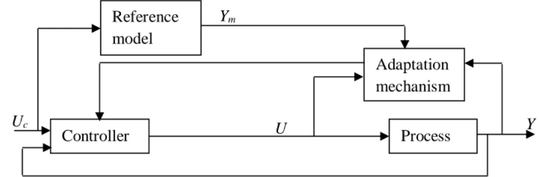
The first MRAS was proposed by Whitaker in 1958 to solve the problem of servomechanisms. The original scheme proposed by Whitaker is shown in Figure 1.7.
The desired performances are formulated by the reference model which gives the desired response to the control signal.
The entire control system has a first ordinary loop containing the reference model and the regulator parameter adjustment mechanism.
The two new ideas brought by the MRAS are: the performances are fixed by the choice of a reference model and the adjustment of the parameters of the regulator is based on the error
e =ym-y. Among the approaches used as adjustment mechanisms, we note: - The rules MIT (gradient).
- The function of Lyapunov. - The hyperstability of Popov.
Figure 1.7 Synoptic diagram of an adaptive reference model system.
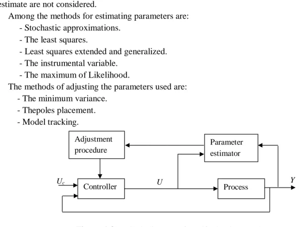
c. Self-adaptive regulator:
In this case of adaptive systems, it is assumed that the regulator parameters are adjusted all the time and follow the process changes. However, it is difficult to analyze the convergence and stability of such systems.
The self-adaptive regulator is based on the idea of separating between the unknown parameter estimator and the adjustment procedure.
Figure 1.8 shows that unknown parameters are estimated online using recursive estimation methods.
The estimated parameters are assumed to take the actual values and the uncertainties of the
Controller Process us Gain-scheduling Uc U Y Controller Process Adaptation mechanism Uc U Y Reference model Ym
12
estimate are not considered.
Among the methods for estimating parameters are: - Stochastic approximations.
- The least squares.
- Least squares extended and generalized. - The instrumental variable.
- The maximum of Likelihood.
The methods of adjusting the parameters used are: - The minimum variance.
- Thepoles placement. - Model tracking.
Figure 1.8 Block diagram of a self-adaptive regulator.
1.4.4.2. Approaches for manipulator arm analysis
The construction of an adaptive reference model system consists of the: 1. Choice of a reference model that definesthe desired performance. 2. Choicee of the control law.
3. Determination of the adaptation law.
If the choice of the reference model and the control law is related to the desired performances, the adaptation law must ensure the stability of the system and the tendency of the error towards zero.
Among the approaches used for the determination of the adaptation law are the gradient approach, the Lyapunov function and the Popov hyperstability.
a. Gradient approach
The gradient method is first used by Whitaker in his original work. The development of this approach towards the MRAS returns to using the rules of MIT.
b. MIT Rule
Let the error be between ym and y (e=ym-y) and θ be the vector of the parameters to be adjusted. A criterion to be minimized is proposed as:
2 2 1 ) ( e J (1.25) Controller Process Parameter estimator Uc U Y Adjustment procedure
13
Therefore, for J to be small it is reasonable to change the parameters in the negative direction of the J gradient i.e :
J dt d (1.26) e dt d .e.
If it is assumed that the parameters θ change more slowly than the other variables of the system, then one can compute e in this case assuming constant θ. e represents the sensitivity of the system and determines the speed of parameters adaptation.
The diagram in Figure 1.9 represents the error model:
Figure 1.9 Error model
The choice of the criterion is arbitrary, if one poses:
Je (1.27)
e e sign(e) (1.28)
The rule of MIT is powerful if is chosen small, but its value may depend on the amplitude of the signal and the gain of the process. As a result, it is not possible to give a limit that ensures the overall stability of the system. The system may be stable for certain values and not for others.
A way to overcome the previous problem is to use the modified MIT rules given by the formula. ) ( ) ( e e e e dt d T (1.29)
Another way to limit the speed of convergence is to introduce the saturation function: . . ) ( ) ( e e e e dt d T sat (1.30)
Sometimes the choice of wide values for y causes instability.
For all these reasons, the choice of an approach that is based on stability seems better. c. Lyapunov function
The extensive research conducted to find a stability analysis method, which ensures the tendency of the error to zero could give the Lyapunov function.
The method proposed by Lyapunov is valid for nonlinear systems and whose idea is illustrated in Figure 1.10.
Π
θ e
14
The statement of the method is as follows: the equilibrium is stable if one finds a real function of the state space, its curve envelopes the state of equilibrium and the derivative of the state variable points to the inside the curve.
Figure 1.10 Illustration of Lyapunov's method
To formally state the results, we consider the following differential equation:
x f( tx, ) , f(0,t)=0 (1.31)
Wherexis a state vector of ndimension.
assumed the function V:Rn1RSatisfying the following conditions: - V(0, t) = 0 for all tR.
- V is differentiable atxandt. - V is positive definite.
The sufficient condition for uniform asymptotic stability for the (1.31) system is:
t V V grad t x F t x V T ( , ) ( ) ) , ( ( 0 for x ≠ 0) (1.32)
So V must be defined negative:
Condition (1.32) will therefore fix the adaptation law thus ensuring the stability and tendency of the error towards zero.
1.5. Mobile robots
1.5.1. Definition of a mobile robot
A mobile robot is a mechanical, electronic and computer system acting physically on its environment in order to achieve a goal that has been assigned to it. This machine is versatile and able to adapt to certain variations of its operating conditions. It has perception, decision and action functions. Thus, the robot should be able to perform various tasks, in several ways, and perform its task correctly, even if it encounters new unexpected situations.
Currently, the most sophisticated mobile robots are primarily oriented towards applications in variable or uncertain environments, often with obstacles, requiring adaptability to the task.
1.5.2. Wheeled mobile robots
Wheel mobility is the most used mechanical structure. This type of robot provides a displacement with a fast movement but requires relatively flat ground. We distinguish several
x=0
=0
V(x)=cst
X1
15
classes of wheeled robots, mainly by the position and the number of wheels used. We will mention here the four main classes of wheeled robots [32].
1.5.3. Classification of wheeled mobile robots
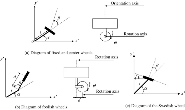
1.5.3.1. Classification according to the type of wheels
In the field of mobile robotics, we find four types of wheels as shown in the Figure 1.11[33]: - Fixed wheels whose axis of rotation passes through the center of the wheels.
- Orientable center wheels, whose axis of orientation passes through the center of the wheels.
- Foolish wheels whose orientation axis does not pass through the center of the wheel.
- Swedish wheels for which the zero component of the sliding speed at the point of contact is not in the plane of the wheel.
Figure 1.11 Diagram of the different wheels types of the mobile platforms 1.5.4. Kinematic modeling
1.5.4.1. Wheel model
Kinematic modeling is the study of the motion of a mechanical system regardless of the forces that influence its motion. At this stage, we are interested only in velocity vectors.
1.5.4.2. Modeling hypothesis
The problem of the control of mobile robots being too vast to be presented exhaustively, in this part a number of simplifying hypotheses:
- The robots are considered rigid and evolving on a plane,
Rotation axis
Rotation axis
(b) Diagram of foolish wheels.
Rotation axis Orientation axis
(a) Diagram of fixed and center wheels.
16
- The robots are equipped with conventional wheels: the point of contact between the wheel and the ground is reduced to a point and the wheel is subjected to rolling constraint without sliding.
1.5.4.3. Rolling without slip and non-holonomy
Many mechanical systems are subject to position and/or velocity constraints, i.e., several relationships between the positions and/or velocities of different points of the system must be satisfied throughout the motion. These constraints are said to be holonomic if it is possible to integrate them and they lead to algebraic relations linking the configuration parameters. These relationships can be eliminated by appropriate change of variables and the system is said to be holonomic. In other words, the robot ability to move from a position to any direction is called holonomic. In the case of non-integrable constraints, the elimination is no longer possible and the system is said to be non-holonomic.
In the case of wheeled robots, these kinematic constraints result from the assumption of rolling without sliding. Consider a vertical wheel that rolls without sliding on a flat ground, the rolling without sliding translates to the zero velocity of point I of the wheel in contact with the ground [34].
Figure 1.12 Description of a wheel
With the notation in Figure 1.12, we obtain:
) ))( cos sin ( ( ) / (I R0 xi yj k i j rk v 0 ) sin ( ) cos ( x r i y r j
Where r is the radius of the wheel and (x, y) is the coordinate of the point o1 in the fixed reference R0(o,i,j,k). We deduce two constraints:
0 sin 0 cos r y r x (1.33)
The model (1.33) can be transformed to make appear the components of the velocities in the planes of the wheel and perpendicular to the wheel, the following kinematic constraints are then obtained: 0 cos sin sin cos y x r y x
17
It is interesting to note that by introducing vr the rolling speed of the wheel and w
its speed of rotation around the axis k, we form the following model:
qS(q)u w v y x 1 0 0 0 sin cos , w v u (1.34)
1.5.4.4. Kinematic model of unicycle wheel robots (differential)
The kinematic model (1.34) of the wheel subjected to rolling without sliding constraints have certain characteristics. One of the characteristics of these non-holonomic systems is that the linearized system is not controllable whereas the real system is.
We consider the mobile robot type unicycle schematically in Figure 1.13, this robot is equipped with two independently controlled fixed-wheel drive and foolish wheels ensuring its stability [34].
Figure 1.13 UnicycleRobot type
Let the abscissa and the ordinate (x, y) of the middle of the axis of the two driving wheels, the orientation of the robot, r the radius of the wheels and 2R the distance between the two drive wheels. By taking again the equation (1.33) and one can easily show that the constraints of rolling without sliding of each of the driving wheels are written:
– For the left wheel
xRcosr1cos 0 (1.35)
yRsinr1sin 0 (1.36)
– For the right wheel
xRcosr2cos0 (1.37)
yRsinr2sin 0 (1.38)
These four constraints are not independent since the difference of the left-hand side of equalities (1.35) and (1.37) is proportional to that associated with (1.36) and (1.38). For example, the last constraint can be omitted. In addition, the constraint is completely integrable. Indeed, we have:
x y
18 2 1 sin cos sin cos r R y x r R y x
So, do one gets:
) ( 2Rr 21 Which implies: constant ) ( 2Rr 21
Consequently, there remain only two independent constraints, (1.35) and (1.36), that are written as: w v y v x sin cos (1.39) Where
– The linear speed of the robot is
( 1 2)
2
r
v (1.40)
– The angular velocity of the robot is
( 2 1) 2 R r w (1.41)
The fact that this system is the same as the model (1.34) obtained for a single wheel (unicycle), which justifies the qualifier term unicycle often used in the literature.
1.5.5. Dynamic model of unicycle wheeled robots
By ignoring the mass of the wheels, the equations of motion can be derived using Euler-Lagrange method as M(q)qC(q,q)qE(q)CT(q) (1.42) Where , cos sin cos 0 sin 0 2 I m d dm dm dm m dm m M l r b b E r sin cos sin cos 1
Where m is the robot mass, I the moment of inertia of the robot about its center of mass,
, 0 0 0 sin 0 0 cos 0 0 dm dm C
19
d the distance between the center of mass and the center of the wheel axle, r the wheel radius R
half distance between the two wheels, l, r the motor torques on the wheels and the constraint force.
By differentiating (1.34), one getsqSuSu. Then by substituting q into (1.42), pre-multiplying by ST, and using the propertySTCT 0, one can have
u(STMS)1ST(MSCS)u(STMS)1STE (1.43)
1.6. Properties and Control of a mobile robot
1.6.1. Definitions,PropertiesandLinearization Definition 1.1 : Lie Derivative [35]
Let h:Dn , f :Dn n then the Lie derivative ofh,with respect to thevector field fis given as
) ( ) ( f x x h x h Lf
Used earlier to find V(x)
) ( ) ( ) ( g x x x h L x h L Lg f f ) ( ) ( ) ( ) ( 2 f x x x h L x h L x h L Lf f f f Example ) ( 2 1 ) (x x12 x22 h , ) 1 ( ) ( 2 1 2 1 2 x x x x x f , 2 2 1 2 2 2 1 1 ) ( x x x x x x x g
(1 ) ) 1 ( ) ( ) ( 2 22 12 1 2 1 2 2 1 x x x x x x x x x f x h x h Lf
( ) ) ( ) ( 12 22 2 2 1 2 2 2 1 1 2 1 x x x x x x x x x x x g x h x h Lg Second-order Derivatives ) ( ) (x x12 x22 h Lg
2( ) 2 ) ( ) ( ) ( 2 12 22 1 2 2 2 2 1 1 2 1 2 x x x x x x x x x x x g x x h L x h Lg g
2 (1 ) ) 1 ( 2 ) ( ) ( ) ( 2 22 12 1 2 1 2 2 1 x x x x x x x x x f x x h L x h L Lf g g 20 Definition 1.2 : Lie Bracket [35]
Let the vectors fields f,g:Dnnthen the Lie Bracket of f and g is found to be
,
( ) ( ) g(x) x f x f x g x g f Example ) 1 ( ) ( 2 1 2 1 2 x x x x x f , 2 1 ) ( x x x g
2 1 2 1 2 1 2 1 2 1 2 ) 1 ( 2 1 1 0 1 ( 1 0 0 1 ) ( ) ( ) ( , x x x x x x x x x x g x f x f x g x g f 2 2 1 2 0 x x Definition 1.3 : Diffeomorphism [35]Let f :Dnn, is said to bea diffeomorphism on D (local diffeomorphism)if: 1- f is continuously differentiable on D
2- f-1 (inverse) existand continuously differentiable, such that
D x x x f f1( ( )) ,
The function f is said to be a global diffeomorphism if in addition 1 -
2 -
im x f(x) Lemma
Let f :Dnn
•Be continuously differentiable on D, and
• If the Jacobian matrix Df f is nonsingular at a pointx0D. Then f is a diffeomorphism in subsetD.
Definition 1.4 : Distribution (Differential Geometry) [35]
A finite set of vectors S
x1,x2,...xp
in n is said to be linearly dependent if there exist a corresponding set of real numbers
i , not all zero, such that0 ... 2 2 1 1
p p i i ix x x x On the other hand, if
0iixi implies that i 0 for each i, then the set
x is said ito be linearly independent.
Given a set of vectors S
x1,x2,...xp
in n, a linear combination of those vector defines a new vector xn, that is, given real numbers 1,2,...p.,
n