Publisher’s version / Version de l'éditeur:
Proceedings 18th International Conference on Port and Ocean Engineering under Arctic Conditions, POAC'05, 2, pp. 781-791
READ THESE TERMS AND CONDITIONS CAREFULLY BEFORE USING THIS WEBSITE.
https://nrc-publications.canada.ca/eng/copyright
Vous avez des questions? Nous pouvons vous aider. Pour communiquer directement avec un auteur, consultez la
première page de la revue dans laquelle son article a été publié afin de trouver ses coordonnées. Si vous n’arrivez pas à les repérer, communiquez avec nous à [email protected].
Questions? Contact the NRC Publications Archive team at
[email protected]. If you wish to email the authors directly, please see the first page of the publication for their contact information.
NRC Publications Archive
Archives des publications du CNRC
This publication could be one of several versions: author’s original, accepted manuscript or the publisher’s version. / La version de cette publication peut être l’une des suivantes : la version prépublication de l’auteur, la version acceptée du manuscrit ou la version de l’éditeur.
Access and use of this website and the material on it are subject to the Terms and Conditions set forth at
Implementation and Testing of a Thickness Redistribution Model for Operational Ice Forecasting.
Kubat, Ivana; Sayed, Mohamed; Savage, S.; Carrieres, T.
https://publications-cnrc.canada.ca/fra/droits
L’accès à ce site Web et l’utilisation de son contenu sont assujettis aux conditions présentées dans le site LISEZ CES CONDITIONS ATTENTIVEMENT AVANT D’UTILISER CE SITE WEB.
NRC Publications Record / Notice d'Archives des publications de CNRC: https://nrc-publications.canada.ca/eng/view/object/?id=eae3b32a-e450-4bcb-9324-aab6335d9a92 https://publications-cnrc.canada.ca/fra/voir/objet/?id=eae3b32a-e450-4bcb-9324-aab6335d9a92
Proceedings 18th International Conference on Port and Ocean Engineering under Arctic Conditions, POAC’05 Vol. 2, pp781-791, Potsdam, NY, USA, 2005.
IMPLEMENTATION AND TESTING OF A THICKNESS REDISTRIBUTION MODEL FOR OPERATIONAL ICE FORECASTING
I. Kubat1, M. Sayed1, S. Savage2, and T. Carrieres3
1
Canadian Hydraulics Centre, NRC, Ottawa, ON, Canada
2
McGill University, Montreal, Quebec, Canada
3
Canadian Ice Service, Environment Canada, Ottawa, ON, Canada
ABSTRACT
The present paper deals with the implementation and testing of an ice thickness redistribution model, which is intended for operational use by the Canadian Ice Service (CIS). The model, developed by Savage (2002), is briefly reviewed. The emphasis of this paper is on the implementation in a Particle-In-Cell (PIC) ice dynamics formulation. The model accounts for the evolution of distributions of thickness and concentration of ice in response to mechanical deformation. This is accomplished without resorting to discrete ice categories. A method to incorporate ice growth from open water is also discussed. The results indicate that the model produces appropriate behaviour and trends.
INTRODUCTION
The Canadian Ice Service (CIS) has been developing a new thickness redistribution model as part of ongoing enhancements to its ice-forecasting operations. The emphasis in this paper is on thickness redistribution due to mechanical deformation of the ice cover, and implementation within the CIS ice dynamics model. An overview of the ice dynamics model was given by Sayed and Carrieres (1999) and Sayed et al. (2002). One of the main features of that model is the use of a Particle-In-Cell (PIC) approach to model ice advection. In this semi-Lagrangian approach, the ice cover is represented by an ensemble of particles. Each particle carries attributes that describe ice conditions, such as thickness and concentration, and ice velocities. At each time step, ice cover properties are mapped from the particles to an underlying Eulerian grid. The momentum and constitutive equations are then solved over the grid. The
use of the grid makes it possible to employ relatively efficient solvers. The resulting velocities, which are calculated on the grid, are next mapped to the particles. At that stage, the particles are advected in a Lagrangian manner. The PIC approach reduces numerical diffusion associated with advection, thereby yielding accurate ice edge locations and other discontinuities (e.g. ridged zones and open water leads). Additionally, the approach directly keeps track of the history and trajectories of the ice cover. Incorporating ice thickness redistribution in the PIC approach requires a somewhat different treatment from that used in Eulerian formulations. While transport of deformed (e.g. ridged/rubbled) ice and leads is simplified, handling of ice growth from open water poses additional complications. This paper deals with some of the special issues that arise in introducing thickness redistribution in a PIC-based ice dynamics model.
Many of the operational models of ice thickness redistribution have so far been based on the approach of Thorndike et al. (1975). That approach employs probability functions to describe the transfer of ice between thickness categories. The transfer functions are derived from the continuity and energy conservation equations, and through some arbitrary assumptions concerning plausible trends for thickness changes. Implementations of Thorndike et al (1975) conceptual model are usually based on dividing ice thickness into discrete categories. Simplified implementations include a two-category model by Hibler (1979), and separate distribution functions for ridged and level ice by Flato and Hibler (1995).
Pritchard and Coon (1981) developed another approach that categorizes ice types as open water (including new ice), thin, flat, and rubbled. They proposed thickness redistribution functions to account for ice transfer between different categories. In that model, minimum and maximum values of thickness are used to define each ice type. Those values also change with time in order to account for thermal growth. Recently, a number of models departed from using discrete thickness categories. For example, Gray and Morland (1994), Shulkes (1995), Gray and Killworth (1996), and Hapaala (2000) all consider the transfer of ice from level to deformed. Then, formulations are proposed to account for thickness and concentration changes in response to ice cover deformation. The present work follows that general approach. Evolution of the thickness and concentration of the ice cover due to convergence and shear deformation are considered.
THE ICE DYNAMICS MODEL
Movements and deformation of the ice cover are determined by solving the equations of conservation of linear momentum together with the constitutive equations that describe stress-strain rate relationship. Additionally, a Particle-In-Cell (PIC) method is used for ice advection. That method also accounts for conservation of mass. Spherical coordinates are employed in the model. In this section, a brief description
of those governing equations and the solution methods are given. The equations are not listed here because of space limitations, and because they follow standard forms familiar to the ice-forecasting community. More details of the present dynamics model can be found in papers by Sayed and Carrieres (1999), and Sayed et al. (2002). The time dependent conservation of linear momentum equations consider that the ice cover moves under the action of air and water drag, Coriolis force, and water surface tilt. The drag forces are given by quadratic formulas. For the stress-strain rate relationship, the Hibler (1979) viscous plastic formulation is used. In that formulation, viscosity coefficients are chosen to describe an elliptic plastic yield envelope (in principal stress space). Pre-yield, for very small strain rates, is accounted for by introducing very high viscosity to approximate a near-rigid behaviour. Strength of the ice cover also follows Hibler’s formulation, whereby strength depends on ice thickness and concentration as well as a strength parameter P*.
According to PIC formulation, the ice cover is represented by an ensemble of interacting particles that are advected in a Lagrangian manner. Each particle carries a number of attributes including thickness of ridged and level ice, concentration of ridged and level ice area fraction, and mean thickness and concentration. For each time step, the particle velocities are determined by interpolating node velocities of an Eulerian grid. Particles can then be advected. The area and mass of all particles within each grid cell are then averaged to update the thickness and ice concentration at the Eulerian grid nodes. A bilinear interpolation function is used to map variables between the particles and the Eulerian grid.
The numerical solution of the governing equations is implemented using a staggered B-grid. The semi-implicit method of Zhang and Hibler (1997) is used to update the velocities and pressures on the grid.
THE THICKNESS REDISTRIBUTION MODEL
The thickness redistribution model of Savage (2002) accounts for the continuous evolution of the thickness and concentration of ice without resorting to discrete categories. Both convergence and shear deformation of the ice cover are related to the change of thickness and concentration. A brief overview of the model is given in this section of the paper. The total area fraction (or concentration), A of the ice cover is
divided into two parts representing the level (or coherent) ice, Acand deformed ice,
Ar. In addition to the mean thickness of the ice cover h, the level and deformed ice are
assigned thicknesses, hc and hr, respectively. These variables satisfy the following
relationships:
r
c
A
A
A
=
+
(1)A
h
=
A
ch
c+
A
rh
r (2)and energy balance. The increase in the potential energy due to ice deformation is assumed to be a fraction of the mechanical work done by the internal stresses in the ice cover. The yield envelope of Hibler (1979) is employed to calculate the stresses, and consequently, to develop the evolution equations for thickness and concentration. Savage (2002) also used the results of Hopkins’ (1998) simulations of the ridging process to determine the ratio of mechanical work that causes the increase of potential energy of deformed ice. The analysis also considers that ice deforms into rubble or ridges that can reach a maximum thickness, which depends on level ice thickness (e.g. Timco and Burden 1997). Further deformation would cause the rubble or ridges to extend horizontally without an increase in thickness. Hopkins’ (1998) results are also used to determine an asymptotic ratio between the maximum thickness of deformed ice and level ice thickness.
Only a listing of the evolution equations of Savage (2002) is given here. Further discussion of the model can be found in Kubat et al. (2004). The evolution functions
make use of a redistribution function, ψ, and parameter, β, which depends on the
ratio of level ice thickness to deformed ice thickness. The redistribution function is given by
(
)
[
]
⎥ ⎥ ⎥ ⎥ ⎥ ⎦ ⎤ ⎢ ⎢ ⎢ ⎢ ⎢ ⎣ ⎡ ⎥ ⎥ ⎥ ⎥ ⎦ ⎤ ⎢ ⎢ ⎢ ⎢ ⎣ ⎡ ⎟ ⎠ ⎞ ⎜ ⎝ ⎛ − + ⎟ ⎠ ⎞ ⎜ ⎝ ⎛ + − ⎟ ⎠ ⎞ ⎜ ⎝ ⎛ + − − = • • • • • • 2 / 1 2 2 2 1 2 2 1 2 1 1 exp 2 1 e e e e e e e A C A ψ (3)where C is a constant used in Hibler’s (1979) expression for ice pressure, 1
•
e and 2 • e ,
are the principal strain rates, and e is the ratio between the major and minor principle
axes of the ellipse describing the yield envelope. The parameter β is given by
1 − ⎟ ⎠ ⎞ ⎜ ⎝ ⎛ ⎟ ⎠ ⎞ ⎜ ⎝ ⎛ = asym c r asym c r h h h h β (4)
where the subscript asym refers to the asymptotic value. The evolution equations can then be listed as follows
(
β)
ψ η = − + r 1 r A t D A D (5) c + cη=βψ A t D A D (6) ⎥ ⎦ ⎤ ⎢ ⎣ ⎡ − ⎟⎟ ⎠ ⎞ ⎜⎜ ⎝ ⎛ − = 1 1 r c r r r h h A h t D h D ψ β (7)where ice convergence, η, is defined as the sum of the two principal strain rates. It also follows from the above equations (Savage, 2002) that evolution of the total concentration and mean thickness is given by
ψ η = + A t D A D (8), and A h t D h D ψ − = (9)
The evolution equations (equations 5 to 9) are solved for each PIC particle.
GROWTH OF NEW ICE
The present thickness redistribution and ice dynamics models are intended to run in coupled mode to ocean and ice thermodynamics models at the Canadian Ice Service (CIS). In that mode of operation, growth and melt of existing ice as well as growth of new ice from open water will be provided to the present model as input at each time step. It is, therefore, necessary to decide on a strategy to include such thermodynamic growth and melt in the present model.
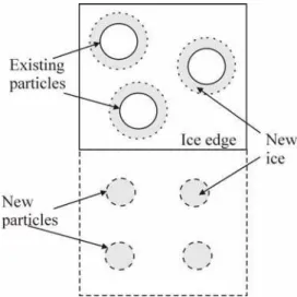
In the present PIC formulation, several particles (typically 10 to 20) usually exist in each grid cell that is occupied by the ice cover. Naturally fewer particles may be present in cells at the ice edge. Each particle in the grid cell carries its own thickness and concentration values for both level and deformed ice. These values may be different for every particle in the same grid cell. Introducing the change of those thickness values due to thermodynamic growth and melt at each time step is straightforward. Growth of ice from open water, however, requires a more complex treatment. There are two cases to consider, as illustrated in Figure 1. The first case corresponds to a grid cell populated with a number of particles. In that case, the volume of new ice is equally distributed among the particles. The new ice is assigned the level ice thickness of the
corresponding particle. Thus the increase in level ice thickness area and the resulting adjustment of area concentrations are carried out for each particle.
Figure 1: Schematic diagram of the growth of ice from open water
The second case corresponds to empty cells, which include no particles (i.e. no ice cover is present). In that case, the volume of new ice in a cell is divided to create four new particles as shown in Figure 1. Four particles are considered a minimum to obtain satistactory interpolation for the PIC model. Tests with more particles did not show discernable differences. Furthermore the new ice is assumed to have a minimum thickness that may be chosen, for example, as 0.05 m. Finally, the new particles are assigned concentration values that are calculated as the area of new ice divided by the area of the cell. We note that the influence of the initial 0.05 m thickness on thermodynamic growth is not tested. Further investigation is needed to clarify the physics of initial ice growth, and sensitivity of the model to the initial thickness.
TEST CASES
Verification of thickness redistribution models is challenging because field measurements are usually sporadic, restricted to narrow geographic locations, and environmental forcing data include many gaps. Recently, however, more complete field observations are becoming available, such as new measurements over the Gulf of St. Lawrence by Prinsenberg (2004). Considering the uncertainties associated with field observations, we examine idealized cases of ice cover deformation as a first step in validating the present model. Those cases make it possible to test the formulation and implementation of the model, and examine trends of the results. Kubat et al. (2004) reported on tests that showed that the model produces expected trends. In this paper, we present results, which focus on the evolution of non-uniform thickness distribution and the behaviour of new ice growth. Such non-uniform thickness distributions are significant because of their relevance to field observations.
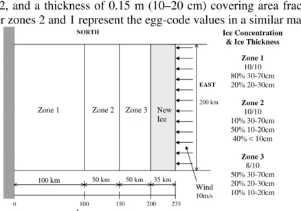
The present test case considers steady wind driving an ice cover against a straight shoreline. The wind acts in a perpendicular direction to the shoreline, and both the shoreline and ice cover are assumed to extend over a large distance. Therefore, movements and deformation take place in a uniaxial manner. This test case resembles conditions observed during field measurements of the LIMEX project (Drinkwater 1989, and Tang and Yao 1992). The initial ice cover is divided into three regions, each having initial conditions according to values given by the egg-code of an ice chart. Figure 2 gives a schematic of the initial ice cover conditions. Only one test case is presented here since it adequately illustrates the performance of the model within space limitations of the paper. Results from other test cases can be found in Kubat et al. (2004). Full documentation of the tests has been given by Kubat and Sayed (2003).
In addition to the initial ice cover, a region extending 35 km to the East of the ice edge is considered to generate new ice due to freeze-up of open water. The rate of growth of new ice from open water was taken as 0.05m/day. The values of parameters used in the test case are as follows: time step = 5 minutes, grid cell size =
5 km, wind speed = 10 m/s, air drag coefficient = 0.002, water drag coefficient = 0.005, and ice rheological properties (for Hibler’s yield conditions)-ice strength, P* =
104 Pa, elliptical yield envelope axes ratio, e = 2, Constant (Eq. 3) C = 20.
The initial conditions, shown in Figure 2, include a number of values of level ice thickness in each zone based on the egg-code values from the ice charts. The total concentration for zone 3 is 8/10 (or 0.8), which is divided into three thicknesses of level ice: a constant thickness of 0.5 m (the average of 30–70 cm given by the ice chart) covering area fraction of 0.5, a thickness of 0.25 m (20–30 cm) covering area fraction of 0.2, and a thickness of 0.15 m (10–20 cm) covering area fraction of 0.1. Conditions for zones 2 and 1 represent the egg-code values in a similar manner.
Ice Concentration & Ice Thickness
Zone 1 10/10 80% 30-70cm 20% 20-30cm Zone 2 10/10 10% 30-70cm 50% 10-20cm 40% < 10cm Zone 3 8/10 50% 30-70cm 20% 20-30cm 10% 10-20cm EAST 0 100 150 200 235 km 200 km NORTH 50 km 50 km 100 km
Zone 1 Zone 2 Zone 3
35 km
New Ice
Wind
10m/s
Figure 2: Initial ice conditions for the test case
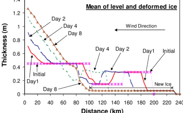
The profiles of the resulting mean ice thickness (of level and deformed ice) and the thickness of deformed ice are shown in Figures 3 and 4. The profiles of total concentration and deformed ice concentration are shown in Figures 5 and 6. As expected, the pressure varies from zero at the ice edge, and increases towards the West to reach a maximum at the land boundary. Strain rates are also largest at the land boundary, which corresponds to larger convergence of the ice cover, and consequently more thickness build-up. The peaks in figures indicate ice deformation at the interface of different zones with different ice thickness and concentration. After approximately 5 days of steady wind action, ice thickness reaches certain limiting values, and no further deformation occurs. An exception, to the trend of increasing thickness towards the land boundary, is the relatively large deformation that occurs in the vicinity of the interface between zones 2 and 3. This large deformation is caused by the low thickness in zone 2.
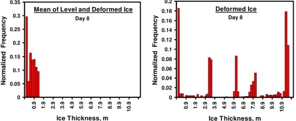
Ice thickness histograms covering the entire test area are shown in Figure 7. The distributions are obtained by considering the values associated with each particle (in this case over the entire test area). The number of particles needed for the PIC formulation is usually adequate to obtain such distributions over relatively small
areas. The histograms illustrate the manner in which thickness distribution evolves over the test period. The “large” bar corresponding to a small thickness (0.05m) represents new ice that grows from open water. A secondary peak shows the thickness changes of that ice.
0 0.2 0.4 0.6 0.8 1 1.2 1.4 0 20 40 60 80 100 120 140 160 180 200 220 240 Distance (km) Thickness (m)
Day 4 Day 2 Day1 Day 8
Day 4 Day 2
Day1 Day 8
Mean of level and deformed ice
Wind Direction
Initial
Initial
New Ice
Figure 3: Profiles of mean ice thickness (mean of level and deformed ice)
0 2 4 6 8 10 12 0 20 40 60 80 100 120 140 160 180 200 220 240 Distance (km) Thickness (m) Day 8 Day 4 Day 2 Day 1 Deformed ice
Figure 4: Profiles of deformed ice thickness
CONCLUSIONS
The preceding presentation examined the implementation of the ice thickness redistribution model of Savage (2002). The model accounts for the evolution of thickness and concentration in response to deformation of the ice cover. In the Particle-In-Cell (PIC) implementation, each grid cell may contain several values of level and deformed ice thickness and concentration. The model determines the evolution of the spectrum of thickness and concentration values for each grid cell. The model, therefore, differs from the class of two-category models that deal with a single mean thickness of ice for each grid cell (Note that the term two-categories is usually used to refer ice and open water).
0 0.2 0.4 0.6 0.8 1 1.2 0 20 40 60 80 100 120 140 160 180 200 220 240 Distance (km) Concentration Day 4 Day 1 Day 2 Day 8
Mean of level and deformed ice
Initial
Figure 5: Profiles of total ice concentration
0 0.02 0.04 0.06 0.08 0.1 0.12 0 20 40 60 80 100 120 140 160 180 200 220 240 Distance (km) Concentration Day 4 Day 1 Day 2 Day 8 Deformed ice
Figure 6: Profiles of deformed ice concentration
0 0.05 0.1 0.15 0.2 0.25 0.3 0.35 -0.1 0.9 1.9 2.9 3.9 4.9 5.9 6.9 7.9 8.9 9.9 10.9 11.9 Ice Thickness, m Normalized Frequency
Mean of Level and Deformed Ice
Day 8 0 0.02 0.04 0.06 0.08 0.1 0.12 0.14 0.16 0.18 0.2 -0.1 0.9 1.9 2.9 3.9 4.9 5.9 6.9 7.9 8.9 9.9 10.9 11.9 Ice Thickness, m Normalized Frequency Deformed Ice Day 8
Figure 7: Histogram of mean and deformed ice thickness covering the entire test area after 8 days
Moreover, the present model accounts for thickness distributions within each grid cell without employing discrete thickness categories. Because each particle carries distinct values of deformed and level ice thickness, a distribution of these values is obtained from each cell. This considerably simplifies the implementation and improves computational efficiency. It should be emphasized that the output of the model covers distributions of thickness, in contrast to the so-called two-category formulations.
The main advantage of the model, however, may be that it is based on few simple assumptions concerning the balance between mechanical work and potential energy, and the dependence of the maximum thickness of deformed ice on level ice thickness. Both assumptions are based on field observations, and the reliable values for the associated parameters are obtained from available discrete element simulations. A test case was presented to examine the evolution of thickness redistribution for an ice cover driven against a shoreline under the action of steady wind. The initial ice cover includes partially variable thickness and concentration distributions. It was chosen to resemble conditions observed during the LIMEX field experiment. The results indicate that the model predicts the expected trends. Thickness reaches higher values near the shoreline, where pressure has the larger values. The thickness grows until a maximum thickness value of deformed ice is reached (depending on the associated level ice thickness). Afterwards, wind forcing may only increase the thicknesses, which are lower than that maximum value. For the present test case, deformation stopped after five days of steady wind forcing. The resulting extent agrees with observations.
The present paper also introduced an approach for dealing with the thermodynamic growth of new ice from open water. This approach appears to avoid potential problems resulting from the typically very small thickness values that are generated at each time step (for example at half-hour intervals). Further investigation is needed to determine the appropriate values for initial new ice. We note that choosing such an arbitrary thickness is the current practice in the multi-year models (value of the smallest thickness category).
REFERENCES
Drinkwater, M.R. (1989). “LIMEX’87 ice surface characteristics: implications for B-band SAR backscatter signatures,” IEEE Transactions on Geoscience and Remote
Sensing, Vol. 27, No. 5, pp.501-513.
Flato, G.M., and Hibler III, W.D. (1995). “Ridging and strength in modeling the thickness distribution of Arctic sea ice”, J. Geophys. Res., Vol.100 (C9), pp. 18,611- 18,626.
Gray, J.M.N.T. and Morland, L.W. (1994). “A two-dimensional model for the dynamics of sea ice”. Philos. Trans. R. Soc. London. A, 347, pp 219-290.
Gray, J.M.N.T. and Killworth, P.D. (1996). “Sea ice ridging schemes”. J. Phys.
Oceanogr. Vol. 26, pp. 2,420-2,428.
Haapala, J. (2000). “On the modelling of ice-thickness redistribution”. J. Glaciology. 46, pp. 427-437.
Hibler III, W.D. (1979). “A dynamic thermodynamic sea ice model,” J. Physical
Oceanography, Vol. 9, No. 4, pp. 815-846.
Hopkins, M.A. (1998). “Four stages of pressure ridging.” J. Geophys. Res., Vol. 103 (C10), pp. 21,883- 21,891.
Kubat, I., and Sayed, M. (2003). “Testing of ice thickness redistribution model,”
Report CHC-TR-016, Canadian Hydraulics Centre, National Research Council, Ottawa, Ontario, Canada, K1A 0R6, July 2003.
Kubat, I., Sayed, M., Savage, S., and Carrieres, T. (2004). “Implementation and testing of a thickness redistribution model for operational ice forecasting,” , Proc.
Int. Offshore and Polar Eng. Conf., ISOPE, Toulon, France, May 23-28, pp.
855-862.
Prinsenberg, S.J., (2004). Personal communication.
Pritchard, R.S., and Coon, M.D. (1981). “Canadian Beaufort sea ice
characterization,” Proc. The 6th Int Conf. On Port and Ocean Eng. Under Arctic
Conditions (POAC 81), Quebec, Canada, July 27-31, Vol II, pp.609-618.
Savage, S.B. (2002). “Two category sea-ice thickness redistribution model,” Report
prepared for Canadian Ice Service, Environment Canada, 373 Sussex Dr, Ottawa, Ontario, Canada, K1A 0H3, March 31, 2002.
Sayed, M., and Carrieres, T. (1999). “Overview of a new operational ice forecasting model”, Proc. Int. Offshore and Polar Eng. Conf., ISOPE, Brest, France, May 30- June 4, Vol. II, pp. 622-627.
Sayed, M., Carrieres, T., Tran, H. and Savage, S.B. (2002). “Development of an operational ice dynamics model for the Canadian Ice Service,” Proc. Int. Offshore
and Polar Eng. Conf., ISOPE, Kitakyushu, Japan , May 26-31, pp. 841-848.
Shulkes, R.M.S.M. (1995). “A note on the evolution equations for the area fraction and the thickness of a floating ice cover”. J. Geophys. Res. Vol. 100 (C3). Pp. 5,021-5,024.
Tang, C.L., and Yao, T. (1992). “A simulation of sea-ice motion and distribution off Newfoundland during LIMEX, March 1987,” Atmosphere-Ocean, Vol. 30, No.2, pp. 270-296.
Thorndike, A.S., Rothrock, D.A., Maykut, G.A., and Colony, R. (1975). “The thickness distribution of sea ice”, J. Geophys. Res., Vol.80, pp. 4,501-4,513.
Timco, G.W., and Burden, R.P., (1997). “An analysis of the shapes of sea ice ridges”,
Cold Reg. Sci. Technol., Vol. 25(1), pp. 65-77.
Zhang, J and Hibler, WDIII (1997). “On an efficient numerical method for modelling sea ice dynamics,” J. Geophysical Research, Vol. 102, No. C4, pp. 8691-8702.