HAL Id: hal-01514134
https://hal.archives-ouvertes.fr/hal-01514134
Submitted on 9 Jun 2021
HAL is a multi-disciplinary open access
archive for the deposit and dissemination of
sci-entific research documents, whether they are
pub-lished or not. The documents may come from
teaching and research institutions in France or
abroad, or from public or private research centers.
L’archive ouverte pluridisciplinaire HAL, est
destinée au dépôt et à la diffusion de documents
scientifiques de niveau recherche, publiés ou non,
émanant des établissements d’enseignement et de
recherche français ou étrangers, des laboratoires
publics ou privés.
Event-Triggered Stabilizing Controllers Based on an
Exponentially Decreasing Threshold
Fairouz Zobiri, Nacim Meslem, Brigitte Bidégaray-Fesquet
To cite this version:
Fairouz Zobiri, Nacim Meslem, Brigitte Bidégaray-Fesquet. Event-Triggered Stabilizing Controllers
Based on an Exponentially Decreasing Threshold.
EBCCSP 2017 - 3rd IEEE Conference on
Event-Based Control Communication and Signal Processing, May 2017, Funchal, Portugal. pp.1-8,
�10.1109/EBCCSP.2017.8022821�. �hal-01514134�
Event-Triggered Stabilizing Controllers Based on
an Exponentially Decreasing Threshold
Fairouz Zobiri
Univ. Grenoble Alpes Laboratoire Jean Kuntzmann
and GIPSA-lab F-38000 Grenoble, France.
Email: [email protected]
Nacim Meslem
Univ. Grenoble Alpes GIPSA-lab
F-38000 Grenoble, France. Email: [email protected]
Brigitte Bidegaray-Fesquet
Univ. Grenoble Alpes Laboratoire Jean Kuntzmann
F-38000 Grenoble, France. Email: Brigitte.Bidegaray@
univ-grenoble-alpes.fr
Abstract—In this paper, we introduce a new policy defining
a stabilizing event-based controller for linear time-invariant systems. The plant operation is divided into two phases, a transient phase and a steady-state regime. In transient regime, we define a Lyapunov-like function; a positive definite function that vanishes only at the origin. However, while a regular Lya-punov function is decaying in time, the LyaLya-punov-like function is allowed to increase, provided that it remains bounded, in order to get larger inter-event times. An upper threshold is thus fixed in the form of an exponentially decaying function, the rate of decay of which is set by solving a generalized eigenvalue problem. In the vicinity of the steady state, the Lyapunov function is prevented from increasing in time to ensure a faster convergence with less control updates.
I. INTRODUCTION
Even though most controllers are meant to be imple-mented on digital platforms, a common practice consists in designing a continuous-time controller first. The resulting control signal is then sampled in order to be converted from an analog to a digital form. A high-frequency sampling is usually used so as to maintain the properties of the control signal and to avoid aliasing, resulting in a large amount of moving data. However, this is not always efficient, especially if the data is propagating through a communication net-work with a limited bandwidth and several interconnected systems.
Event-based control strategies have been developed as a response to these design concerns. In event-based control, the control loop is closed only when a variable of the system, state or other, violates a predefined condition on proper behavior, designated by the term event-triggering condition. A zero-order hold (ZOH) is then applied between two sampling instants.
Different control methods find their event-based counter-parts in the literature. In [1], an event-based PID controller is introduced, whereas [2] suggests an event-based output-feedback approach. More advanced control strategies such as model predictive control [3] and H∞control [4] are also being explored in an event-triggered operation mode.
In this work, we address the problem of stabilizing a linear time-invariant (LTI) system by means of an event-triggered state-feedback controller. Several authors have
already worked on the question of feedback stabilization. For example, in [5] the author plans the execution of the control task when an error norm becomes too large in comparison with the state norm. In [6], Sontag’s general feedback stabilization formula has been extended to the case of event-based control under the assumption that a Control Lyapunov Function exists. A novel direction is taken in [7], where instead of using a ZOH between two events, a copy of the model generates continuously a control law using an estimated state. This way, the sensors send the measured state to the controller only when an event occurs. In [8], the authors have devised an algorithm that keeps the Lyapunov-like function of the system enclosed between the Lyapunov functions of two auxiliary systems. In this paper we also adopt an approach that relies on a Lyapunov-like function, that is forced to remain below an exponen-tially decaying function that we define. Thus, we avoid the need to define auxiliary systems and we reduce the complexity of the problem, as the auxiliary systems are of the same order as the plant.
The use of an exponential threshold function has origi-nated in [9] and can also be found in [10] and [11]. The only difficulty in this approach is to find a suitable decay rate for the exponential envelope function. As one of the main contributions of this paper, we manage to prove that the problem of finding the said decay rate can be expressed as a generalized eigenvalue problem, a class of problems for which many tools have been developed.
This approach also differs from the above methods and from the one in [8] in that it uses two different event-triggering strategies. At first, in transient time, the proce-dure described above is adopted. When a neighborhood of steady-state is reached, we force the time derivative of the Lyapunov function to remain negative, thus ensuring a faster asymptotic convergence in less executions of the control task.
This paper is divided as follows. Section II lays out the basic formulation of the problem and introduces the concepts that we use in the rest of the paper. The event-based control algorithm is described in section III, where we also provide the proofs of the stability of the
event-based control system and the existence of a minimum inter-sample time. In section IV we test the method on a numerical example. Finally, in section V, we compare the results given by this method to three other event-based strategies found in the literature.
II. PROBLEMDEFINITION
Let us define a LTI control system of the form ˙
x(t ) = Ax(t) + Bu(t), x(t0) = x0, t0= 0,
(1) where x(t ) ∈ Rn is the state vector, u(t ) ∈ Rm is the control signal, A and B are matrices of the corresponding dimensions.
We consider the pair (A,B) to be controllable, thus guar-anteeing the existence of a linear state feedback of the form
u(t ) = −K x(t). (2)
The feedback gain K is designed to render the matrix (A − BK ) Hurwitz, resulting in a globally asymptotically stable closed-loop system.
The event-based control signal u(t ) is piecewise constant, updated only when the triggering conditions are satisfied. Therefore, at times tk (k ∈ N) when an event occurs
u(tk) = −K x(tk). (3)
Otherwise, at times t ∈]tk, tk+1[ when the system provides
a desirable performance
u(t ) = u(tk). (4)
We have seen in [12] that a constant event-triggering con-dition achieves only practical stability. We know from [13] that asymptotic stability is achieved through a decaying-in-time triggering condition.
The motivation behind this work is to improve the approach described in [8]. From that approach, we keep the idea of a locally increasing Lyapunov-like function that remains bounded. However, in this work, we introduce an alternative method for keeping the Lyapunov-like function bounded from above, without the need for defining reference systems (see [8]).
III. SCHEDULING OF THECONTROLTASK
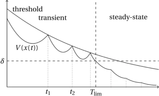
As mentioned earlier, in this paper we split the imple-mentation of our event-based controller into two parts. First, in transient time, we define a threshold function that will serve as an upper limit to the Lyapunov-like function of the event-based system. Then, in steady-state, we shift our focus on the time derivative of the Lyapunov function, by making sure it never becomes positive.
We will show later that it makes more sense to formally define the limits of the transient and steady-state regime in terms of the threshold function that we introduce below. For now we define the transient regime as all time instants
threshold
V (x(t ))
t1 t2 Tlim
transient steady-state
δ
Fig. 1. An illustrative example of the behavior of the Lyapunov-like function in transient and steady state regimes.
t such that t < Tlim (Tlim> 0). The steady state consists
thus of all time instants t , such that t ≥ Tlim. An illustrative
example of this approach is given in Fig. 1. A. The Triggering Conditions in Transient Time
We define V :Rn→ R+, the Lyapunov-like function asso-ciated with system (1), as
V (x) = x(t)TP x(t ), (5)
where P ∈ Rn×n is a symmetric positive definite matrix, solution to the equation
(A − BK )TP + P(A − BK ) = −Q. (6)
In classical control, stability necessitates V to be decreasing in time. However, as proved in [12], if we allow V (x) to be locally increasing, the stability property can be maintained with an event-triggered control law. Moreover, this allows to obtain events that are sparser in time. For this reason, it becomes necessary to define a positive decreasing upper bound for V (x(t )). The instants at which V (x(t )) reaches the upper bound will serve also as our triggering events.
1) Defining the Threshold Function: Let W :R+→ R+ be a scalar function, such that for all t
dW (t )
d t < 0, (7)
and
V (x(t )) ≤ W (t). (8)
At t = tk, when the feedback loop is closed and u(t ) is
given by equation (3), the time derivative of (5) takes the following form dV (x) d t |t =tk= x(tk) T((A − BK )TP + P(A − BK ))x(t k) = −x(tk)TQ x(tk). (9)
Letλmax(−Q,P) be the maximum generalized eigenvalue of
the pair (−Q,P),
and P1/2 be the symmetric square-root of P . Then, from [14]
λmax(−Q,P) = −λmin(P−1/2QP−1/2), (11)
λmin(P−1/2QP−1/2) being the minimum eigenvalue of
P−1/2QP−1/2, in the traditional sense of eigenvalue.
There-fore, from equation (9) dV (x(t ))
d t |t =tk≤ λmax(−Q,P)V (x(t)). (12)
Extrapolating equation (12) for t > tkwe obtain a first order
linear differential inequality, which yields dV (x(t ))
d t ≤ V (x0)e
−α(t −t0), (13)
thus providing a suitable upper threshold function
W (t ) = V (x0)e−αt. (14)
The coefficientα is selected such that 0 < α < −λmax(−Q,P)
in order to enforce the condition given by equation (8). We can now describe the event-triggered strategy.
Theorem 1. Let V (x) be the function given by equation
(5), and W (t ) be the decaying exponential function given by equation (14). The time instant tk+1 (k ∈ N) is defined as
tk+1= inf{t > tk, V (x(t )) = W (t)}.
Then, at time t = tk+1, the event-triggered control law
defined in equations (3) and (4) renders system (1) stable. Proof. Since W (t ) is exponentially decreasing toward zero, it is enough to show that V (x(t )) is always lower than W (t ). We need to show that whenever V (x(t )) = W (t), V (x(t)) is pushed back below W (t ). Such is the case at t0, where
W (0) = V (x0), and is also the case for every tk (k ∈ N).
At t = tk and from equation (12)
−x(tk)Q x(tk) ≤ λmax(−Q,P) V (x(tk).
But, since at instant t = tk, V (x(tk)) = W (tk), we can re-write
the last equation as
−x(tk)Q x(tk) ≤ λmax(−Q,P) W (tk) < −αW (tk). In other words, at t = tk dV (x(t )) d t |t =tk< dW (t ) d t |t =tk, V (x(tk+)) < W (tk+).
Then, we can deduce that lim
t →∞V (x(t )) ≤ limt →∞W (t ) = 0. (15)
This proves that updating u(t ) to −K x(tk) at t = tk,
stabi-lizes the system.
The problem now is to find a suitable α.
We have a special interest in finding the maximum possible value ofα, in order to be able to satisfy a trade-off between the number of transmissions and the smoothness behavior of the system.
2) Finding the Decay Rate α: In what follows, we shall drop the arguments P and Q and designate the maximum eigenvalue of the pair (P,Q) simply as λmax.
Equation (12) can be re-written as x(tk)T((A − BK )TP +P(A − BK ))x(tk)
≤ −λmax x(tk)TP x(tk).
(16) λmax is the solution of the following optimization problem
minimize − λ subject to
(A − BK )TP + P(A − BK ) ≤ −λP P > 0
(17)
This problem is quasiconvex and there exist many works devoted to its solution in the literature, among which we can cite [14] and [15].
B. Steady-state Triggering Conditions
We demand a stronger control effort in the neighborhood of steady-state. In that case, we can require that time derivative (9) remain negative. This will drive the state to equilibrium position, from which it is harder to deviate, thus spreading the controls further in time.
Theorem 2. Let V (x) be the function given by equation (5)
and satisfying equation (9). The time instants tk+1 (k ∈ N) are defined as tk+1= inf ½ t > tk, dV (x(t )) d t = 0 ¾ .
Then, at time t = tk+1, the event-triggered control law
defined in equations (3) and (4) renders system (1) stable. Proof. Since dV (x(t ))d t is guaranteed to remain negative by the triggering conditions, the plant is stable.
C. Defining Tlim
We define Tlim as the time when V (x(t )) reaches a
predefined small value (δ > 0).
Tlim= min {t |V (x(t )) = δ} . (18)
We know that for all t , V (x(t )) ≤ W (t), hence we can give an upper bound for Tlimas
Tlim≤ min {t |W (t ) = δ} =−1
α ln δ V (x0)
. (19)
D. Minimum Inter-sample Time
Up to now, we have managed to prove asymptotic stability of the event-based plant. However, the plant has to remain stable for at least some minimum time span after tk, that we refer to as τmin> 0. The existence of this
τmin is important, as it prevents the need for an infinite
number of updates in a finite interval of time.
Before we prove the existence of such a minimum time, let us introduce the following lemma.
Lemma 1. For all ε < pδ/λmax(P ), there exists τ1
inde-pendent of k such that for all t ∈ (tk, min(tk+ τ1, tk+1)),
kx(t )k ≥ ε.
Proof. Let us first estimate kx(tk)k.
Since λmin(P )kx(tk)k2≤ V (x(tk)) ≤ λmax(P )kx(tk)k2, and in
transient timeδ ≤ V (x(tk)) ≤ V (x0), we have
s δ λmax(P )≤ kx(tk)k ≤ s V (x0) λmin(P ) ,
where λmin(P ) and λmax(P ) are the minimum and
maxi-mum eigenvalues of P , respectively. We cast equation (1) as
˙
x(t ) = (A − BK )x(t) − BK ∆kx(t ), (20)
where ∆kx(t ) = x(tk) − x(t). The solution to equation (1) is
Lipschitz, and therefore there exists a constant Lx such that
k∆kx(t )k ≤ Lx(t − tk). Then the integral form for equation
(20) is x(t ) = e(A−BK )(t−tk)x(t k) − Z t tk e(A−BK )(t−s)B K∆kx(s)d s.
Since A − BK is Hurwitz, we can bound kx(t)k from below kx(t )k ≥ kx(tk)k − L(t − tk )2 2 BK ≥ s δ λmax(P )− L (t − tk)2 2 BK ,
where · is the subordinated matrix norm.
Therefore, for sufficiently small t , say t −tk< τ1and 0 < ε <
p
δ/λmax(P ), we can guarantee that kx(t)k ≥ ε.
Theorem 3. There exists a minimum time delay τmin> 0
independent of k, such that for all k ∈ N, tk+1− tk> τmin.
Even though this result is valid in transient and steady state regimes, we will give the proof for the transient time only. The proof for the steady state is given in [16]. Proof. The proof follows the same scheme as in [12] but here the problem is simpler as we do not attempt to track a reference signal that may contain discontinuities.
Before time tk+1, we know that dV (x(t ))/d t necessarily vanishes. We will find a minimum time delay, τ2,
indepen-dent of k, lower than τ1 on which dV (x(t ))/d t remains
negative. It will necessarily be lower than the desired τmin.
From equation (20) we can easily deduce that V (x(t ))
d t = −x(t )
T
Q x(t ) − 2∆kx(t )TKTBTP x(t ).
We now suppose that tk < t < tk+ τ1. According to
Lemma 1 −x(t )TQ x(t ) ≤ −λmin(Q)ε2=: −β. We also have k − 2∆kx(t )TKTBTP x(t )k ≤ 2k∆kx(t )TkKTBTP kx(t)k ≤ 2Lx(t − tk)KTBTP s V (x0) λmin(P ) . For 0 < τ2< τ1, this can be rendered lower than β/2 and
hence dV (x(t ))/d t < −β/2 < 0. This τ2 can be chosen as
τmin.
IV. SIMULATIONRESULTS
In this section we test the validity of the approach on a numerical example. For this, we consider the following second order linear system
˙ x(t ) = · 0 1 −2 3 ¸ x(t ) + · 0 1 ¸ u(t ), (21) where x(t ) =£ x1(t ) x2(t ) ¤T.
The initial state x0 is given as
x0=£ 1 −1 ¤ .
The linear feedback control law is chosen (for a conver-gence time of 3 seconds) as
u(t ) =£
−1.7329 −5.6667 ¤ x(t).
We associate to the system a quadratic Lyapunov-like function, as described by (5), with a first time derivative given by equation (9).
In this work, to find P , Q, the decay rate α and W (t), we solve the maximum generalized eigenvalue problem using the ’gevp’ command of Matlab, which is based on the algorithms in [15]. This command relies on the formulation of problem (17) as linear matrix inequalities (LMI) using the LMI declaration tools of the Robust Control Toolbox. We obtain as a result P = · 12.1917 4.3548 4.3548 3.2660 ¸ , Q = · 32.5123 11.6128 11.6128 8.7089 ¸ . The solver gives a value of λmax = 2.6653. So we pick
α = 2.3. We also set δ = 0.01 and W (0) = 10.5437. We have simulated the behavior of the system for 8 seconds (both transient and steady state included), and we have chosen a sampling period of 10−4 s, resulting in 8 × 10⁴ time units. The choice to sample at such high frequency is motivated by the fact that detecting the exact moment at which V (x(t )) intersects with W (t ) is impossible in a discrete-time simulation, and thus we try to emulate continuous-time behavior as close as possible.
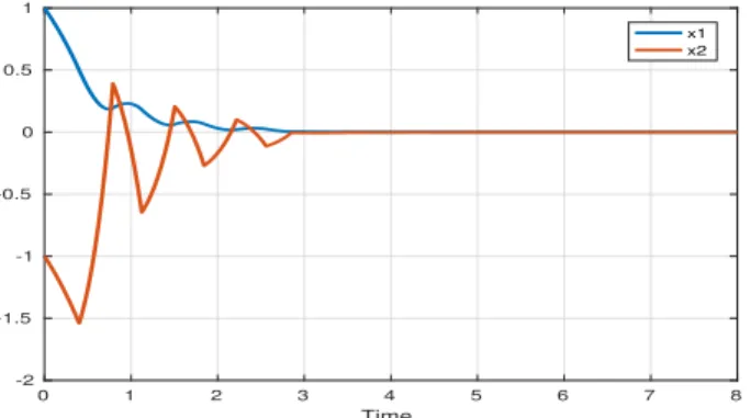
Fig. 2 represents the evolution of the states, x1(t ) and
x2(t ) in time. It shows that even though the response is
not quite smooth in transient time, the oscillations are not exaggerated and die out quickly. The states converge to the equilibrium point at zero in 3 seconds: Tlim= 3.16.
Fig. 3 represents the event-based control law. The control signal is updated only 16 times for 80, 000 time
0 1 2 3 4 5 6 7 8 Time -2 -1.5 -1 -0.5 0 0.5 1 x1 x2
Fig. 2. The time evolution of the states of the event-based system.
units, i.e, we have reduced the number of samples by a factor of 1/5000 compared to a periodic implementation. This result is illustrated better through Fig. 4, where the intersections between the pseudo-Lyapunov function and the envelope function W (t ) represent the events.
In Fig. 3, we notice that even if the updates of the control are distant in time, they occur, on average, at a regular pace. The reason for this is the linearity and time-invariance of the system, which make for a predictable behavior.
0 1 2 3 4 5 6 7 8 Time -4 -2 0 2 4 6 8 control signal
Fig. 3. The piecewise constant event-based control law.
0 1 2 3 4 5 6 7 8 Time 0 2 4 6 8 10 12 V(x) W(t)
Fig. 4. The time evolution of the Lyapunov-like function along with the exponentially decaying upper threshold function.
Note that after each event, the Lyapunov function is sent back to a decreasing state, proving the stability of the
scheme.
In steady state, after t = 3s, the norm of the state vector drops to a very small value, and therefore, it would be hard to see the events on the curve of the derivative of the Lyapunov function. For this reason we propose a graph of the distribution of the events for the entire simulation interval, as given by Fig. 5. It shows that in steady state, we do in fact obtain less updates than if we had kept the same triggering conditions for the entire simulation interval. 0 1 2 3 4 5 6 7 8 Time 0 0.2 0.4 0.6 0.8 1 1.2 1.4 1.6 1.8 2
Fig. 5. The distribution in time of the events in transient and steady-state regimes.
Remark 1. In continuous time, an event is detected when
V (x(t )) = W (t). However, as the simulation is run in discrete time, this equality is impossible to detect. Instead we detect the instants at which V (x(t )) ≥ W (t).
As in that case, there is no guarantee that an update of u(t ) will send V (x(t )) below W (t ), we propose the following update at t = tk
W (tk) = V (x(tk)).
It is perfectly possible to do so, as W (t ) is a fictitious function and does not correspond to any actual data. Additionally, this update corresponds to continuous-time behavior.
This way, we render the system robust to impulsive distur-bances.
Remark 2. At t = 0, we choose to set W (0) > V (x0), as
a safety measure. This is not really necessary as we have proved that the case when W (0) = V (x0) is well handled by
the algorithm. Therefore, for t ∈ [t0, t1[, W (t ) = W (0)e−αt;
whereas for k ≥ 1 and t ≥ tk, W (t ) = V (tk)e−α(t −tk).
V. COMPARISON WITHOTHERMETHODS
In this section we compare the performances of the method described above with other event-based control methods. We have chosen three methods from the literature and we will compare them in terms of number of updates of the control law and in terms of quality of the performance. The first method that we explore is the one developed in [5]. Since this method has been primarily developed for nonlinear systems and is based on the existence of an
Input-to-State Stable (ISS) Lyapunov function, we refer to it as the ISS method.
The second method that can be found in [6], relies on an extension of Sontag’s stabilization formula and for nonlin-ear systems, requires the existence of a Control Lyapunov Function (CLF). For this reason, we refer to it as the CLF method.
Finally, the method of [8] is based on reachability analysis and therefore is referred to as the rechability method. To describe these methods, we keep the notations used up to now in this paper.
A. The ISS Method
As said previously, this method relies on the existence of an ISS Lyapunov function. However, for the simpler linear case, this property is satisfied as long as the plant is controllable.
For the linear case, the event-triggering scheme ensures that
kx(t ) − x(tk)k ≤ σkx(t)k, ∀t (22)
where 0 < σ < 1. If this condition is satisfied for all t, dV (x(t ))/d t < 0, thus guaranteeing stability. In order to perform the comparaison, we have tested our method and the ISS method uder the same conditions, the ones stated in section IV.
The parameter σ is chosen such that
λmin(Q) > σkKTBTP + PBK k, (23)
where λmin(Q) is the smallest eigenvalue of Q (Q, P , B
and K are the same as the ones defined in the previous sections of this article). Condition (23) yields a value σ = 0.05.
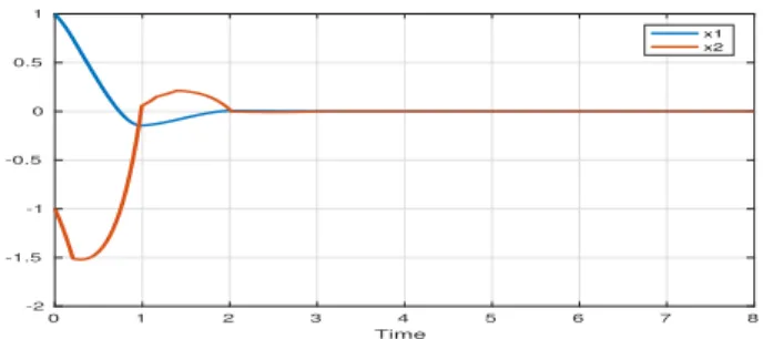
Fig. 6 represents the evolution of the states of system (21). We can notice that the response is of good quality and does not exhibit any oscillations as ours does. However, such good quality comes at a price, as this implementation required 356 updates of the control law for 80, 000 sampling instants. This is a relatively high number compared to our 16 updates for the same simulation interval.
If we use the control law developed by the author of this method in [5], the number of updates is reduced to 176, but is still very large compared to our results.
B. The CLF method
This method proves that it is possible to extend Sontag’s stabilizing formula to event-based systems in the existence of a CLF.
Again the existence of a CLF is guaranteed in the linear case by the controllability of the plant. The event-based algo-rithm detects the time instants when the Lyapunov function is not decreasing enough. Some smoothness considerations are also added to the triggering conditions.
In the linear case, this method translates into an optimal
0 1 2 3 4 5 6 7 8 Time -1.5 -1 -0.5 0 0.5 1 x1 x2
Fig. 6. The time evolution of the states as obtained through the ISS method.
control problem, for which we need to introduce the following weighting matrices on the state and the control respectively Q = · 2 0 0 2 ¸ , R = 1 12.
To find P , a Riccati equation of the form P A + ATP − R−1P B BTP = −Q is solved. We have obtained a value of
P = · 3.2743 0.2743 0.2743 0.7743 ¸ .
Fig. 7 represents the evolution of the states of plant (21). It shows that the quality of the response is relatively good. For a simulation interval of 8 seconds, it requires 22 updates of the control law.
Even though our approach has required less samples, for
0 1 2 3 4 5 6 7 8 Time -2 -1.5 -1 -0.5 0 0.5 1 x1 x2
Fig. 7. The time evolution of the states as obtained through the CLF method.
a simulation of 8 seconds, the difference is not significant. The advantage of our method appears in the long run. As we run the simulation for 30 seconds, our method requires 45 samples, while the CLF method needs about the double (85 samples).
C. The Reachability Method
In this method, a Lyapunov-like function, similar to the one we describe, is associated to the plant. This function is then forced to remain framed between the decaying Lyapunov functions of two auxiliary systems, a slow and a fast system. An event is generated when the pseudo-Lyapunov function intersects with either the upper or lower threshold.
of the event-based implementation, we have decided to omit it in our analysis. The speed of the slow system has been decreased by a factorβs= 0.95 compared to the
event-based system, and is of the following form ˙
xs(t ) = βs(A − BK )xs(t ),
where xs(t ) ∈ Rn is the state of the slow system, which is is
in closed-loop for all t .
This value ofβshas been chosen after sweeping the interval
of definition of βs, ]0, 1[, and noticing that the method
yields better results as βs gets closer to 1. For the rest, we
have kept the parameters of section IV.
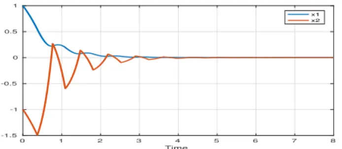
The response is shown in Fig. 8. As expected, the quality
0 1 2 3 4 5 6 7 8 Time -1.5 -1 -0.5 0 0.5 1 x1 x2
Fig. 8. The time evolution of the states as obtained through the reachability method.
of the response is similar to ours, as the two methods work on the same principle. The reachability method needed 22 samples for an 8 seconds simulation.
The reachability method also requires the definition of extra systems, thus increasing the complexity of the imple-mentation as the order of the plant increases. Conversely, our method requires the introduction of a simpler scalar function, regardless of the order of the system.
VI. CONCLUSION
This work introduces two new concepts to the event-based stabilization of an LTI system. First, in order to further decrease the number of calls to the controller, different strategies are adopted for the transient regime and for the steady-state regime. For both regimes, the fact that the triggering conditions consist in a single scalar function renders the implementation straightforward. The parameters of this scalar function can easily be derived from the data of the problem, using numerical methods readily available in the mathematical literature and software packages.
The second contribution of this paper consists in an explicit solution to the problem of determining the speed of con-vergence. Writing the problem as a famous optimization problem has allowed us to optimize the system’s conver-gence speed, while developing two different approaches for the two operation regimes maximized the time between two events.
One drawback of this method is the lack of smoothness of the response in transient time, due to the oscillations
experienced by the Lyapunov-like function. There is a range of applications for which this might not be suitable, but the category of applications for which this approach is designed are those that do not require high precision and are not sensitive to oscillations and abrupt changes. Moreover, our main objective is to drastically decrease the number of times the control task is applied.
The algorithm does not include the cases where distur-bances are acting on the various parts of the control loop, or when the emission or reception of signals experiences time delays. These can nonethless be seen as areas of expansion for future works.
Additionally, the simplicity of the approach renders it easily adaptable to the case of nonlinear plants, as another idea to explore.
ACKNOWLEDGMENT
This work has been partially supported by the LabEx PERSYVAL-Lab (ANR-11-LABX-0025-01).
REFERENCES
[1] K.-E. Årzén, “A simple event-based PID controller,” in IFAC World
Congress, Beijing, China, Jul. 1999.
[2] M. Donkers and W. Heemels, “Output-based event-triggered control with guaranteed L-infinity gain and improved event-triggering,” 49th
IEEE Conference on Decision and Control, 2010.
[3] A. Ferrara, A. N. Oleari, S. Sacone, and S. Siri, “An event-triggered Model PredictiveControl scheme for freeway systems,” 51st IEEE
Conference on Decision and Control. Maui, Hawaii, USA, December
2012.
[4] A. Selivanov and E. Fridman, “Event-triggered H∞control: A switch-ing approach,” IEEE Transactions on Automatic Control, vol. 61, no. 10, pp. 3221 – 3226, October 2016.
[5] P. Tabuada, “Event-triggered real-time scheduling of stabilizing con-trol tasks,” IEEE Transactions on Automatic Concon-trol, vol. 52, no. 9, pp. 1680–1685, 2007.
[6] N. Marchand, S. Durand, and J. F. G. Castellanos, “A general formula for event-based stabilization of nonlinear systems,” IEEE Transactions
on Automatic Control, vol. 58, no. 5, pp. 1332–1337, 2013.
[7] D. Lehmann and J. Lunze, “Event-based control: A state-feedback approach,” in 2009 European Control Conference. IEEE, Aug. 2009, pp. 1716–1721.
[8] N. Meslem and C. Prieur, “Event-based controller synthesis by bound-ing methods,” European Journal of Control, vol. 26, pp. 12–21, 2015. [9] X. Wang and M. Lemmon, “On event design in event-triggered
feedback systems,” Automatica, vol. 47, pp. 2319–2322, 2011. [10] R. Postoyan, P. Tabuada, D. Nesic, and A. Anta, “A unifying
Lyapunov-based framework for the event-triggered control of nonlinear sys-tems,” 50th IEEE Conference on Decision and Control and European
Control Conference, 2011.
[11] ——, “A framework for the event-triggered stabilization of nonlinear systems,” IEEE Transactions on Automatic Control, vol. 60, no. 4, pp. 982–996, April 2015.
[12] F. Zobiri, N. Meslem, and B. Bidégaray-Fesquet, “Event-based sam-pling algorithm for setpoint tracking unsing a state-feedback con-troller,” in Second International Conference on Event-Based Control,
Communications, and Signal Processing. Krakow, Poland: IEEE, Jun.
2016.
[13] C. Stöcker and J. Lunze, “Input-to-state stability of event-based state-feedback control,” 2013 European Control Conference (ECC), Zurich,
Switzerland, July 2013.
[14] S. Boyd and L. E. Ghaoui, “Method of centers for minimizing generalized eigenvalues,” Linear Algebra and its Applications, vol. 188 -189, pp. 63 – 111, July - August 1993.
[15] Y. Nesterov and A. Nemirovskii, Interior-Point Polynomial Algorithms
in convex programming, ser. Studies in Applied and Numerical
[16] A. Seuret, C. Prieur, and N. Marchand, “Stability of nonlinear systems by means of event-triggered sampling algorithms,” IMA Journal of
Mathematical Control and Information, vol. 31, no. 3, pp. 415–433,