HAL Id: hal-03197111
https://hal.archives-ouvertes.fr/hal-03197111
Submitted on 15 Apr 2021
HAL is a multi-disciplinary open access
archive for the deposit and dissemination of
sci-entific research documents, whether they are
pub-lished or not. The documents may come from
teaching and research institutions in France or
abroad, or from public or private research centers.
L’archive ouverte pluridisciplinaire HAL, est
destinée au dépôt et à la diffusion de documents
scientifiques de niveau recherche, publiés ou non,
émanant des établissements d’enseignement et de
recherche français ou étrangers, des laboratoires
publics ou privés.
and OH: results from QUANTIFY
P. Hoor, J. Borken-Kleefeld, D. Caro, O. Dessens, O. Endresen, M. Gauss, V.
Grewe, D. Hauglustaine, I. Isaksen, P. Jöckel, et al.
To cite this version:
P. Hoor, J. Borken-Kleefeld, D. Caro, O. Dessens, O. Endresen, et al.. The impact of traffic
emis-sions on atmospheric ozone and OH: results from QUANTIFY. Atmospheric Chemistry and Physics,
European Geosciences Union, 2009, 9 (9), pp.3113-3136. �10.5194/acp-9-3113-2009�. �hal-03197111�
www.atmos-chem-phys.net/9/3113/2009/ © Author(s) 2009. This work is distributed under the Creative Commons Attribution 3.0 License.
Chemistry
and Physics
The impact of traffic emissions on atmospheric ozone and OH:
results from QUANTIFY
P. Hoor1, J. Borken-Kleefeld2, D. Caro3, O. Dessens4, O. Endresen5, M. Gauss6, V. Grewe7, D. Hauglustaine3, I. S. A. Isaksen6, P. J¨ockel1, J. Lelieveld1, G. Myhre6,8, E. Meijer9, D. Olivie10, M. Prather11, C. Schnadt Poberaj12, K. P. Shine13, J. Staehelin12, Q. Tang11, J. van Aardenne14, P. van Velthoven9, and R. Sausen7
1Max Planck Institute for Chemistry, Dept. of Atmospheric Chemistry, 55020 Mainz, Germany 2Transportation Studies, German Aerospace Center (DLR), Berlin, Germany
3Laboratoire des Sciences du Climat et de l’Environment (LSCE), CEN de Saclay, Gif-sur-Yvette, France 4Centre for Atmospheric Science, Dept. of Chemistry, Cambridge, UK
5DNV, Det Norske Veritas (DNV), Oslo, Norway 6Dept. of Geosciences, University of Oslo, Norway
7Deutsches Zentrum f¨ur Luft- und Raumfahrt, Inst. f¨ur Physik der Atmosph¨are, Oberpaffenhofen, 82234 Wessling, Germany 8Center for International Climate and Environmental Research-Oslo (CICERO), Oslo, Norway
9Royal Netherlands Meteorological Institute, KNMI, De Bilt, The Netherlands 10Meteo France, CNRS, Toulouse, France
11Department of Earth System Science, University of California, Irvine, USA
12Institute for Atmospheric and Climate Science, Swiss Federal Institute of Technology, Z¨urich, Switzerland 13Department of Meteorology, University of Reading, UK
14Joint Research Center, JRC, Ispra, Italy
Received: 9 July 2008 – Published in Atmos. Chem. Phys. Discuss.: 21 October 2008 Revised: 5 May 2009 – Accepted: 5 May 2009 – Published: 14 May 2009
Abstract. To estimate the impact of emissions by road,
air-craft and ship traffic on ozone and OH in the present-day atmosphere six different atmospheric chemistry models have been used. Based on newly developed global emission in-ventories for road, ship and aircraft emission data sets each model performed sensitivity simulations reducing the emis-sions of each transport sector by 5%.
The model results indicate that on global annual average lower tropospheric ozone responds most sensitive to ship emissions (50.6%±10.9% of the total traffic induced per-turbation), followed by road (36.7%±9.3%) and aircraft ex-hausts (12.7%±2.9%), respectively. In the northern upper troposphere between 200–300 hPa at 30–60◦N the max-imum impact from road and ship are 93% and 73% of the maximum effect of aircraft, respectively. The latter is 0.185 ppbv for ozone (for the 5% case) or 3.69 ppbv when scaling to 100%. On the global average the impact of road even dominates in the UTLS-region. The sensitivity of ozone formation per NOx molecule emitted is highest for aircraft exhausts.
Correspondence to: P. Hoor
The local maximum effect of the summed traffic emissions on the ozone column predicted by the models is 0.2 DU and occurs over the northern subtropical Atlantic extending to central Europe. Below 800 hPa both ozone and OH respond most sensitively to ship emissions in the marine lower tropo-sphere over the Atlantic. Based on the 5% perturbation the effect on ozone can exceed 0.6% close to the marine surface (global zonal mean) which is 80% of the total traffic induced ozone perturbation. In the southern hemisphere ship emis-sions contribute relatively strongly to the total ozone pertur-bation by 60%–80% throughout the year.
Methane lifetime changes against OH are affected strongest by ship emissions up to 0.21 (± 0.05)%, followed by road (0.08 (±0.01)%) and air traffic (0.05 (± 0.02)%). Based on the full scale ozone and methane perturbations pos-itive radiative forcings were calculated for road emissions (7.3±6.2 mWm−2) and for aviation (2.9±2.3 mWm−2). Ship induced methane lifetime changes dominate over the ozone forcing and therefore lead to a net negative forcing (−25.5±13.2 mWm−2).
1 Introduction
The rise in energy consumption by the growing human pop-ulation and the increasing mobility are associated with emis-sions of air pollutants in particular by road and air traffic as well as international shipping. These emissions are expected to increase in future, affecting air quality and climate (Kahn Ribeiro et al., 2007) which in turn affects air pollution lev-els (Hedegaard et al., 2008). The impact of air traffic emis-sions has been subject of various investigations (e.g. Hidalgo and Crutzen, 1977; Schumann, 1997; Brasseur et al., 1996; Schumann et al., 2000) also assessing projections for the fu-ture (e.g. Sovde et al., 2007; Grewe et al., 2007). For the present day atmosphere these studies indicated an increase of ozone of 3–6% due to aircraft emissions in the region of the North Atlantic flight corridor. More recent studies cal-culated an overall maximum effect of 5% for the year 2000 in the northern tropopause region (Grewe et al., 2002). De-pending on season the values typically range between 3 ppbv and 7.7 ppbv in January and September, respectively (Gauss et al., 2006). The global annual averaged radiative forcing due to the additional O3from air traffic is estimated to be of the order of 20 mW/m2(Sausen et al., 2005).
Relatively few studies have dealt with the impact of road traffic (Granier and Brasseur, 2003; Niemeier et al., 2006; Matthes et al., 2007), and ship emissions (Lawrence and Crutzen, 1999; Corbett and Koehler, 2003; Eyring et al., 2005; Dalsoren and Isaksen, 2006; Endresen et al., 2007; Eyring et al., 2007). Endresen et al. (2003) reported peak ozone perturbations of 12 ppbv for the marine boundary layer during northern summer over the northern Atlantic and Pa-cific regions. Eyring et al. (2007) used a multi-model ap-proach based on EDGAR emissions and reported somewhat lower values of 5–6 ppbv for the North Atlantic. They also calculated a maximum column perturbation of 1 DU for the tropospheric ozone column associated with radiative forcings of 9.8 mW/m2. For road emissions Matthes et al. (2007) found maximum contributions to surface ozone peaking at 12% in northern midlatitudes during July. Similar values of 10% are reported by Niemeier et al. (2006) for current con-ditions.
Besides the effects of pollutants on ozone a potential change of the OH concentration is of importance in partic-ular for regional air quality and the self-cleaning capacity of the atmosphere (Lelieveld et al., 2002). Changes of methane loss rates due to anthropogenic emissions are reported to be on the order of 0.5%/yr of which 1/3 (0.16%) is due to an in-crease of OH from anthropogenic CO, NOxand non-methane hydrocarbons (NMHCs) (Dalsoren and Isaksen, 2006). In addition, the regional OH distribution can be differ substan-tially due to the short lifetime of OH and NOxin particular in the lower troposphere and the different response of the HOx-NOx-O3-system to NOxperturbations (Lelieveld et al., 2002, 2004). Although generally the presence of carbon compounds such as CH4, NMHCs, and CO act as a sink for
OH, the latter can be efficiently recycled in the presence of NOx. The reaction of NO with HO2produces O3and recy-cles OH making the system less sensitive to perturbations. Pristine regions with low NOxand high OH concentrations conditions are favourable for OH-formation following ozone production from NOx-perturbations. Since emissions from the three transport sectors are emitted into rather different en-vironments their impact on O3and OH may differ strongly.
The EU-project QUANTIFY (Quantifying the Climate Impact of Global and European Transport Systems) is the first attempt to provide an integrated and consistent view on the effects of traffic on various aspects of the atmosphere. Fuglestvedt et al. (2008) calculated that transport accounts for 31% of the man made ozone forcing since preindustrial times. Here we present simulations obtained with six differ-ent models all using the same set of emissions to provide a credible evaluation of the present-day atmospheric effects by traffic and to estimate the uncertainties of model results. This study focuses on the global impact of traffic exhaust emis-sions on the current chemical state of the atmosphere. The climatological implications and future projections are sub-ject of followup studies.
2 Emissions and simulation setup
Emissions for the three transport sectors road, shipping and air traffic were replaced in the EDGAR data base with re-spect to the individual emission classes and recalculated sep-arately for QUANTIFY. Emissions from road transportation were developed bottom-up: Vehicle mileage and fleet aver-age emission factors were estimated for the year 2000. The inventory differentiates between five vehicle categories and four fuel types and covers 12 world regions and 172 coun-tries. It is adjusted for the year 2000 to the national road fuel consumption (Borken et al., 2007, and references therein) or national statistics or own calculations. National emissions are allocated to a 1◦×1◦-grid essentially according to popu-lation density with emissions from motorised two- and three-wheelers biased towards agglomerations and emissions from heavy duty vehicles biased towards rural areas. The emis-sions used in this study are based on a draft version (Borken and Steller, 2006). The final inventory for road traffic in-cludes improved emission factors. With fuel consumption and CO2 emissions only 3% higher, the final global traf-fic emissions of NOx, NMHC and CO are higher by 33%, 48% and 51%, respectively. The integrated annual emissions which were used in this study for selected species had to use the draft emissions and are given in Table 1.
The emissions for ship traffic were reconstructed for QUANTIFY based on fuel- and activity-based esimates by Endresen et al. (2007). They report a fuel consumption be-ing about 50–80 Mt (≈ 70–80%) lower than in Eyrbe-ing et al. (2005) or Corbett and Koehler (2003). They attribute the dif-ference to the different assumptions for the operation at sea.
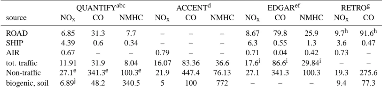
Table 1. Emissions from different sources provided by QUANTIFY for the year 2000 in TgN NOxand TgC CO and NMHC, respectively (for NMHCs the conversion of 161/210 according to TAR was used). Soil and biogenic isoprene emissions were taken from Ganzeveld et al. (2006); Kerkweg et al. (2006), biogenic emissions of hydrocarbons and CO according to von Kuhlmann et al. (2003a,b).
QUANTIFYabc ACCENTd EDGARef RETROg
source NOx CO NMHC NOx CO NMHC NOx CO NMHC NOx CO ROAD 6.85 31.3 7.7 – – – 8.67 79.8 25.9 9.7h 91.6h SHIP 4.39 0.6 0.34 – – – 6.3 0.55 1.3 3.6 0.47 AIR 0.67 – – 0.79 – – 0.71 0.04 0.42 0.73 – tot. traffic 11.91 31.9 8.04 16.07 83.36 36.6 17.6i 86.6i 29.84i – – Non-traffic 27.1e 341.3e 100.3e 21.9 447.4 76.13 27.1 341.3 100.3 19.3 275.6 biogenic, soil 6.89j 48.2 340.5 5 100 772 – – – 9.4 77.3
aRoad emissions: Borken and Steller (2006),bShip emissons: Endresen et al. (2007),cAircraft emssions: Eyers et al. (2004),dEmission inventory developed within ACCENT (Atmospheric Climate Change: The European Network of Excellence) and GEIA (Global Emissions Inventory Activity), evan Aardenne et al. (2005); Olivier et al. (2005),fShip emissions from Eyring et al. (2005),g Reanalysis of the tropospheric composition over the past 40 years, data taken from report on emissions data sets and methodologies for estimating emissions, ftp://ftp.retro.enes.org/pub/documents/reports/D1-6 final.pdf,hTotal land based traffic,iIncluding non-road land transport,jGanzeveld et al. (2006); Kerkweg et al. (2006)
For further details see Endresen et al. (2007).
Aircraft emissions are based on the AERO2K dataset (Eyers et al., 2004) including the emissions from military aviation. The emissions for each transport sector are given in Table 1. Non-traffic emissions used in the present modelling exer-cise are based on the latest release of the EDGAR32FT2000 emission inventory (van Aardenne et al., 2005; Olivier et al., 2005) including emissions of greenhouse gases and ozone precursors for the year 2000 with the exception of methane. Methane was prescribed as a surface boundary condition using time dependent surface mixing ratios as in J¨ockel et al. (2006) based on surface observations from the AGAGE database. For the initialization the three dimen-sional methane distribution from the same simulation was used.
For biomass burning monthly means for the year 2000 were used based on GFED estimates with multi-year (1997– 2002) averaged activity data using Andreae and Merlet (2001) and Andreae (2004, personal communication) for NOx emission factors (BB-AVG-AM). Lightning NOx was specified at 5 TgN/year, representing the current best esti-mate (Schumann and Huntrieser, 2007).
NMHCs were subdivided into individual organic and partly oxidized species. The partitioning of the NMHCs was performed according to von Kuhlmann et al. (2003a) and is shown in Table 2 for biomass burning and fos-sil fuel related emissions. The mass of NMHCs given in kg(NMHC)/yr was converted to kg(C)/year using a ratio of 161/210 TgC/Tg(NMHC) for mass(Carbon)/mass(NMHC-molecule) as in the third IPCC assessment report. The specific ratios were then applied to calculate the individual NMHC partitioning.
Table 2. Fraction of individual species contributing to the total
emission of NMHCs from biomass burning and fossil fuel combus-tion in QUANTIFY (von Kuhlmann et al., 2003a,b).
NMHC specifications species biomass burning fossil fuel C2H6 0.1014350 0.05974 C3H8 0.0322390 0.09460 C4H10 0.0416749 0.7154 C2H4 0.1904856 0.03715 C3H6 0.0849224 0.01570 CH3OH 0.1075290 0.01436 CH3CHO 0.0483586 0. CH3COOH 0.1136230 0. CH3COCH3 0.0501278 0.02375 HCHO 0.0609397 0.004787 HCOOH 0.0404954 0. MEK 0.1281699 0.03447
Biogenic emissions for isoprene and NO emissions from soils were also included based on online calculations with the EMAC model (ECHAM5/MESSy, atmospheric chemistry) (Ganzeveld et al., 2006; Kerkweg et al., 2006) for 1998– 2005 as described in J¨ockel et al. (2006). The 5-hourly out-put fields were converted to monthly means and provided as offline fields to all partners. Thus, seasonal cycles are repre-sented in the biogenic fields as well as in the biomass burn-ing emissions and the aircraft emissions, but not for ship and road traffic emissions or in the other EDGAR-based fields.
To compare the emissions provided by QUANTIFY with other projects and data bases some recently used inventories are also given in Table 1. Notably the road traffic emissions are lower than in other inventories. The final road traffic
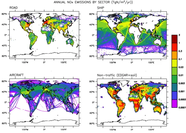
Fig. 1. NOxemissions (TgN/m2/year) used in QUANTIFY by sector.
Table 3. Model simulations performed for QUANTIFY.
experiment emission road ship aircraft
BASE 100% 100% 100%
ROAD 95% 100% 100%
SHIP 100% 95% 100%
AIR 100% 100% 95%
ALL 95% 95% 95%
emissions by Borken et al. (2007) are higher by 33% for NOx and about 50% for CO emissions than those used in this study. Nonetheless, low total CO emissions are a result of lowered average emission factors accounting for effective use of catalytic converters in light duty vehicles.
The resulting source strengths of NOx from the differ-ent sectors, which were used in QUANTIFY are shown in Fig. 1. Globally, road NOxemissions are dominated by the eastern US and western Europe as well as India and east-ern China, the latter with an increase rate of 6%/year (Ohara et al., 2007) only between 2000 and 2003. Besides the conti-nental coast lines in the northern hemisphere and around the major shipping routes ship traffic over the northern central
Atlantic between 25◦–55◦N is a significant source of NOx over a large area. A second NOxsource from ship emissions covering a large area is traffic along the east coast of Asia. Besides the continental eastern US and western Europe the largest emissions from air traffic also occur over the North Atlantic, though further north than the shipping maxima. In the southern hemisphere NOx emissions are largely domi-nated by non-traffic sources and biomass burning.
The simulation period covers the years 2002 and 2003 with 2002 as spin-up. Each participating model calculated the chemical state of the atmosphere for present day condi-tions using all emissions as described above. The perturba-tion simulaperturba-tions were performed by reducing the emission of each individual transport sector by 5% (see Table 3). This relatively small reduction was applied to avoid nonlinear re-sponses of the chemical system which would occur by set-ting the respective emissions to zero. To check for linearity a final simulation was carried out with all transport sectors si-multaneously reduced by 5%. Post processing confirmed the linearity of the small scale perturbation approach allowing to integrate the effects of the individual transport sectors in this setup.
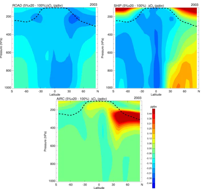
Fig. 2. Comparison of the small perturbation approach (5% emission reduction) and later scaling to a total removal of the respective traffic
emission based on the simulations of p-TOMCAT. The plots indicate the difference of the ozone perturbation from both approaches.
2.1 Small perturbations and scaling
As mentioned above, for this study a small perturbation-approach was chosen for two main reasons: Since one focus of the analysis is a direct comparison of the impact of the differnt emissions, one needs to minimize non-linearities in the chemistry calculations. The total removal of one emis-sion source could lead to responses of the chemical system such that the sum of the effects of each individual transporta-tion sector exceeds the effect of all traffic emission sources switched off simultaneously. Furthermore the unscaled re-sponse of the chemical system is expected to be closer to the effect of realistic emission changes rather than a total emis-sion decline.
We need to emphasize that the small scale approach is fun-damentally different from a 100% perturbation, since non-linearities can lead to significant differences between both approaches. This is illustrated in Fig.2, which shows the dif-ferences of the ozone perturbations from a small perturba-tion approach, which is subsequently scaled to 100% and a 100% decline of the emissions. The sensitivity study was performed by one of the participating models (p-TOMCAT). It clearly shows that depending on the region where the emis-sions occur the effects are very different and can even have opposite signs.
The non-linearity with respect to aircraft emissions is mostly positive throughout the northern upper troposphere (i.e. the scaled small NOx reduction leads to a stronger
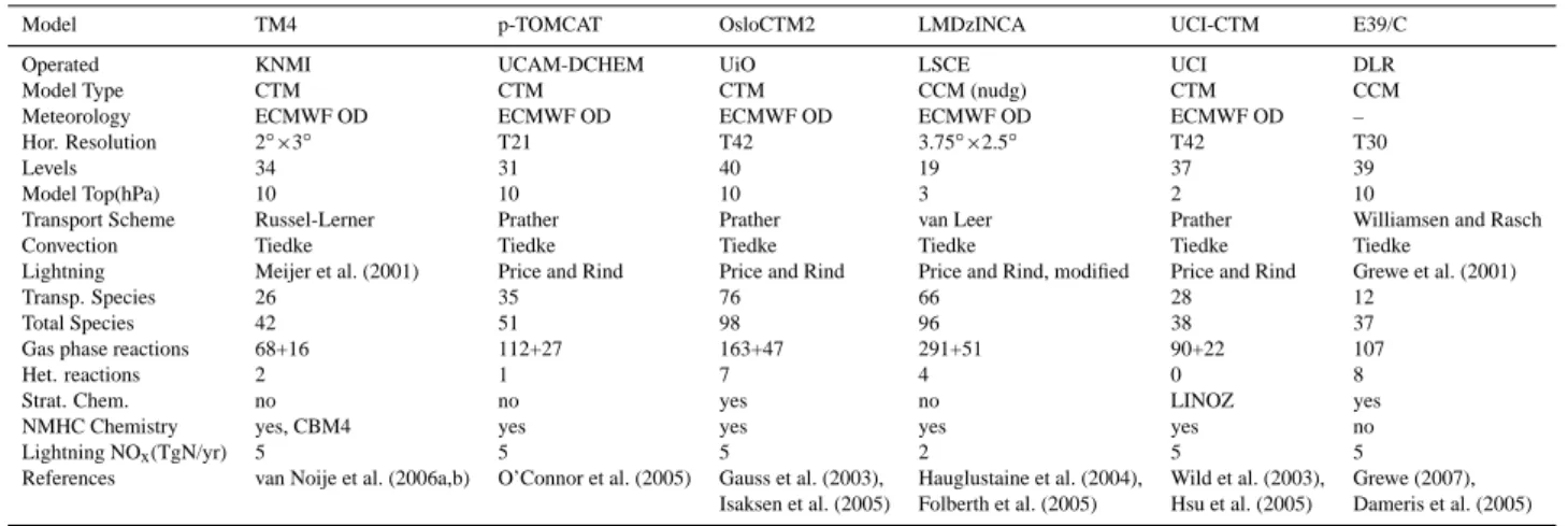
Table 4. Participating models.
Model TM4 p-TOMCAT OsloCTM2 LMDzINCA UCI-CTM E39/C
Operated KNMI UCAM-DCHEM UiO LSCE UCI DLR
Model Type CTM CTM CTM CCM (nudg) CTM CCM
Meteorology ECMWF OD ECMWF OD ECMWF OD ECMWF OD ECMWF OD – Hor. Resolution 2◦×3◦ T21 T42 3.75◦×2.5◦ T42 T30
Levels 34 31 40 19 37 39
Model Top(hPa) 10 10 10 3 2 10
Transport Scheme Russel-Lerner Prather Prather van Leer Prather Williamsen and Rasch Convection Tiedke Tiedke Tiedke Tiedke Tiedke Tiedke
Lightning Meijer et al. (2001) Price and Rind Price and Rind Price and Rind, modified Price and Rind Grewe et al. (2001)
Transp. Species 26 35 76 66 28 12
Total Species 42 51 98 96 38 37
Gas phase reactions 68+16 112+27 163+47 291+51 90+22 107
Het. reactions 2 1 7 4 0 8
Strat. Chem. no no yes no LINOZ yes
NMHC Chemistry yes, CBM4 yes yes yes yes no
Lightning NOx(TgN/yr) 5 5 5 2 5 5
References van Noije et al. (2006a,b) O’Connor et al. (2005) Gauss et al. (2003), Hauglustaine et al. (2004), Wild et al. (2003), Grewe (2007), Isaksen et al. (2005) Folberth et al. (2005) Hsu et al. (2005) Dameris et al. (2005)
response of ozone compared to a total decline of the air-craft NOx-source). The largest difference in that region oc-curs where the aircraft NOx-source is located. As shown by Meilinger et al. (2001) the ozone production efficiency (PO3) in the upper troposphere is at maximum for NOx lev-els around 1 ppbv. At NOxlevels of 0.1–0.3 ppbv, which are typical for this region, PO3 and thus the scaled ozone pertur-bation is more sensitive to a small decrease of NOxthan for a total removal of the aircraft NOxsource.
In contrast, the average effect of road traffic is of opposite sign. As will be shown below its effect on ozone in the upper troposphere can be quite substantial. Since road traffic emis-sions largely occur over the continents in regions with high background pollution and NOx-levels in the ppbv-range, a small reduction of the emission enhances PO3. Therefore the scaled ozone perturbation from the small perturbation is larger than that from the total road perturbation. Verti-cal transport by convection over the continents, particularly during summer, redistributes this ozone perturbation to the tropopause region. It is interesting that the ozone response rather than the NOx-perturbation from road is redistributed via convection in the models.
The sensitivity of ozone perturbations related to ship emis-sions is more complex. In the lower northern hemisphere tro-posphere NOx-levels are generally found to be higher than in the tropics or southern hemisphere. Therefore the northern hemisphere troposphere responds most sensitively to small scale perturbations of the ship emissions.
The sensitivities deduced from p-TOMCAT are most likely at the higher end and differences between both ap-proaches can expected to be smaller based on case studies from other models for individual sectors. Nevertheless one should keep in mind, that the small scale approach is fun-damentally different from a total decline of one emission source.
In the following all perturbations are shown unscaled unless explicitly mentioned.
3 Participating models
Six models were applied to estimate the effect of traffic emis-sions on the current atmospheric chemical composition. Five of them simulated a two years period and included higher or-der chemistry schemes. These five models contribute to the ensemble mean results, which are presented in the follow-ing (TM4, p-TOMCAT, OsloCTM2, UCI and LMDzINCA). One model (E39/C) was used in a different mode to pro-vide information on the interannual variability of the traf-fic impact using a ten year transient simulation. Four mod-els are CTMs using prescribed operational ECMWF data to simulate the meteorological conditions (TM4, p-TOMCAT, OsloCTM2 and UCI). The other two models are coupled CCMs (chemistry climate models). LMDzINCA was nudged to the operational ECMWF fields whereas E39/C was oper-ated as a climate model. Some general properties of the mod-els are listed in Tab. 4. Except for E39/C all modmod-els included explicit NMHC chemistry. The TM4 uses a Carbon Bond Mechanism reaction scheme (CBM4) not including acetone chemistry. Three of the models do not include stratospheric chemistry reactions (TM4, p-TOMCAT, LMDzINCA). The number of species ranged from 42 (TM4) to 125 (LMDz-INCA). LMDzINCA and TM4 used their own biogenic and oceanic emissions, respectively (see below).
3.1 TM4
The KNMI chemistry transport model TM4 (van Noije et al., 2006a,b) is driven by ECMWF analysed meteorology and contains a chemistry scheme derived from the Carbon Bond Mechanism reaction scheme (CBM4) (Houweling et al., 1998). It was run at a horizontal resolution of 2×3 degrees with 34 model levels from the surface up to 10 hPa.
The lightning parameterisation (Meijer et al., 2001) uses convective precipitation from ECMWF to describe the hor-izontal distribution of lightning and normalised profiles
calculated by Pickering et al. (1998) to distribute lightning produced NOxvertically between cloud base and cloud top. Vertical emission profiles were also adopted as included in the respective emission files. In addition to the QUANTIFY emissions oceanic emissions were taken from the POET emission inventory, ammonia emissions from EDGAR 2.0, and volcanic SO2 and DMS (Dimethylsulfide) emissions from the standard model configuration of TM4.
3.2 LMDzINCA
The CNRS-LSCE model, LMDz-INCA had a resolution of 3.75◦ in longitude and 2.5◦ in latitude with 19 levels ex-tending from the surface up to about 3 hPa and is driven by ECMWF operational data (Hauglustaine et al., 2004).
The NMHC setup of the LMDz-INCA model was used. It considers detailed tropospheric chemistry with a com-prehensive representation of the photochemistry of non-methane hydrocarbons (NMHC) and volatile organic com-pounds (VOC) from biogenic, anthropogenic, and biomass burning sources.
Most anthropogenic emissions were taken from the EDGAR3.2FT2000 database. The effective injection height of biomass burning emissions into the atmosphere was taken into account with the emission heights calculated in the RETRO (REanalysis of the TROpospheric chemical compo-sition over the past 40 years) project. The lightning source was determined interactively in LMDz-INCA with a mod-ified Price and Rind (1992) parameterization, and its total was prescribed at ≈ 2. Tg[N]/year. Biogenic sources were calculated with the vegetation model ORCHIDEE. Oceanic emissions were taken from Folberth et al. (2005).
3.3 OsloCTM2
The Oslo CTM2 model is a 3-D chemical transport model driven by ECMWF meteorological data and extending from the ground to 10 hPa in 40 vertical layers. The horizontal resolution for this study was Gaussian T42 (2.8◦×2.8◦). The model was spun up for several years with emissions from the POET and RETRO projects, then for additional 6 months with the emissions provided for the QUANTIFY project. One restart file was archived for March 2002. From this file the five different scenarios were started, which were run for 22 months.
3.4 p-TOMCAT
The model used during the first part of the QUANTIFY project is the global offline chemistry transport model p-TOMCAT. It is an updated version (see O’Connor et al. (2005)) of a model previously used for a range of tropo-spheric chemistry studies (Savage et al., 2004; Law et al., 2000, 1998). Convective transport was based on the mass flux parameterization of Tiedtke (1989). The parametriza-tions includes descripparametriza-tions of deep and shallow convection
with convective updrafts and largescale subsidence, as well as turbulent and organized entrainment and detrainment. The model contains a nonlocal vertical diffusion scheme based on the parameterization of Holtslag and Boville (1993). In this study p-TOMCAT was run with a 5.7o×5.7o hori-zontal resolution and 31 vertical levels from the surface to 10 hPa. The offline meteorological fields used are from the operational analyses of the European Medium Range Weather Forecast model. The chemical mechanism includes the reactions of methane, ethane and propane plus their ox-idation products and of sulphur species, it includes 96 bi-molecular, 16 terbi-molecular, 27 photolysis reactions and 1 heterogeneous reaction on sulphuric acid aerosol. The model chemistry uses the atmospheric chemistry integration pack-age ASAD (Carver et al., 1997) and is integrated with the IMPACT scheme of Carver and Scott (2000). The ozone and nitrogen oxide concentrations at the top model level are con-strained to zonal mean values calculated by the Cambridge 2D model (Law and Nisbet, 1996). The chemical rate coef-ficients used by p-TOMCAT have been recently updated to those in the IUPAC Summary of March 2005. The model parameterizations of wet and dry deposition are described in Giannakopoulos et al. (1999).
3.5 UCI
The UCI CTM is a 3-D eulerian chemistry-transport model driven by meteorological data from the ECMWF IFS version cycle 29r2 at T42L40 (see OsloCTM2). Tropospheric chem-istry is handled by ASAD software package (Carver et al., 1997), containing 38 species (28 transported) and 112 reac-tions (Wild et al., 2003), while in the stratosphere, it employs the stratospheric linear ozone scheme (Linoz) and conducts linear calculations of (P-L) (Hsu, 2004). Photolysis rates are calculated by the Fast-JX package (Bian and Prather, 2002). Transport scheme uses the second order moments (Prather, 1986). Lightning is parameterized with the method of Price and Rind (1992). Convection is simulated, following the ECMWF Tiedtke convection diagnostics.
3.6 E39/C
Impacts by road and ship traffic were provided by DLR based on simulations with E39/C. The perturbation fields are derived as monthly mean values from a transient sim-ulation from 1990 to 1999 (Dameris et al., 2005; Grewe, 2007). The meteorology is calculated by the climate model ECHAM4.L39(DLR) and therefore does not represent an in-dividual year. Nevertheless, it represents the late 20 cen-tury climate and is therefore to some extent comparable to the other simulations of the year 2003. In particular the emissions which were used by the other participating CTMs are different. The impacts are derived using tagging meth-ods (Grewe, 2004) and hence differ from the 5% change approach used by other modelling groups in QUANTIFY.
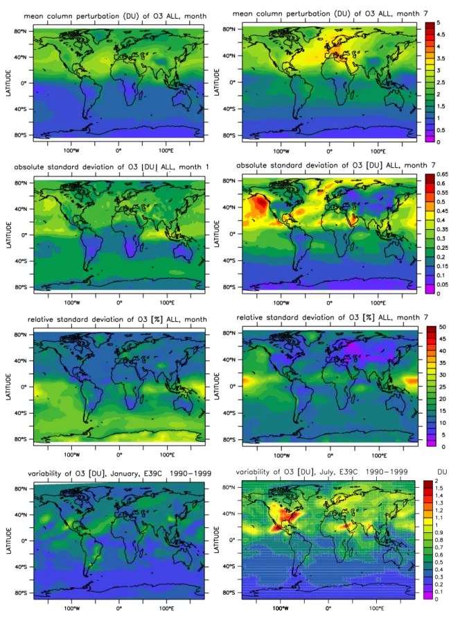
Fig. 3. Mean column ozone perturbations for the integrated emissions from all types of transport obtained from the average of TM4,
LMDzINCA, OSLO CTM2, UCI and p-TOMCAT (top row) for January (left) and July (right). The corresponding absolute and relative standard deviations (relative to the ensemble mean perturbation) are displayed in the second and third row. The lower two panels show the interannual variation of the detrended transportation induced ozone perturbation based on E39/C. Note that the data on display are scaled to 100% to allow the comparison to the interannual variability deduced from E39/C.
Fig. 4. As Fig. 3, but for the zonal mean in ppbv (scaled to 100%). Solid contours show the perturbation relative to the mean unperturbed
simulation and the dashed line indicates the tropopause.
However, both methods try to identify the individual con-tributions from sectors. Changes in the concon-tributions are de-tected comparably by both approaches (Grewe, 2004), i.e. the standard deviation based on interannual variability is sim-ilar for both approaches.
4 Traffic induced ozone changes 4.1 Total ozone perturbation
The integrated effect of the emission reduction (ALL-case) by 5% is shown in Fig. 3 for January and July, respectively. Note that the data in Figs. 3 and 4 are scaled to 100% to allow the comparison to the interannual variability of E39/C
(see below). The column ozone distribution change was inte-grated from the surface up to 50 hPa. The results from E39/C are not included in the calculation of the mean fields since the results of E39/C were obtained with a different setup and a different method.
The mean total ozone perturbations in Fig. 3 exhibit strong hemispheric differences of the traffic emissions with almost zero effect in the southern hemisphere, but maximum effects of about 4 DU during northern hemisphere summer (3 DU during winter). All models simulate a similar location of the strongest ozone perturbation extending from the north-ern subtropical Atlantic to central Europe.
The maximum ozone perturbation is strongest pronounced during northern summer. Interestingly its southern hemi-spheric seasonal cycle – despite being weak – is in phase
with the northern hemisphere with a maximum effect of less than 2 DU. This is most likely due to interhemispheric trans-port and mixing of ship and road emissions occuring during northern summer, which exceed the effects of emissions on the southern hemisphere (see also Fig. 6).
Note furthermore that the effects of traffic emissions over the Pacific and Indian Ocean downwind of the densly popu-lated coastal areas and sources of pollution, are not as strong as over the central Atlantic Ocean. A comparison with the NOx emission distribution (Fig. 1) indicates that over the northern hemispheric Atlantic in particular ship traffic and also aircraft emit large amounts of NOxand that these strong emissions occur over a relatively large area. Over the eastern US and western Europe the sum of all three emission cate-gories reach a maximum. Their combination is responsible for the relatively strong perturbations in these regions.
To assess the robustness of the perturbation signal two tests are performed. First the model to model differences in terms of the associated standard deviation is assessed to esti-mate the impact of model uncertainties. Second, the impact of the chosen meteorology (year 2003) is tested by compar-ing to the interannual variability uscompar-ing the standard devia-tion of the transport signal derived from the transient E39/C simulation, which includes natural variability of the tropo-sphere and the stratotropo-sphere due to variations of ozone in-flux, transport patterns (e.g. induced by El Nino), and others (Grewe, 2007). The inter-model standard deviations (one-σ ) are shown in Fig. 3c–f. Overall the models calculate very similar patterns with a relative standard deviation mostly be-low 15% over large regions of the globe where the effect of the perturbation is strongest. In the southern hemisphere, the relative standard deviations are in general somewhat higher (between 20–30%), since the absolute column perturbations (Fig. 3c and 3d) are not as large as in the northern hemi-sphere. The large absolute deviation over the northern Pacific Ocean during July is caused by the impact of ship emissions, which leads to ozone perturbations ranging from 0.5 DU (TM4) to 2 DU (p-TOMCAT). Largest relative deviations oc-cur over the tropical central Pacific, where perturbations of ozone are relatively low. Thus, small perturbations may lead to relatively large variations between the models. Note how-ever, that calculated ozone perturbations in particular over Europe and the central Atlantic are relatively robust indicat-ing a significant impact of traffic emissions in these regions. To assess the interannual variability of the signal we com-pared the transport induced ozone changes to a ten year tran-sient simulation of E39/C. As can be seen from Fig. 3(bot-tom) the traffic induced perturbation signal simulated by E39/C over the ten years period is on the order of 0.8 DU and 1.2 DU in January and July, respectively. Largest vari-ations occur in coastal regions, where synoptic variability leads to advection of either relatively clean maritime air or air from polluted urban areas. Although the perturbation sig-nal from E39/C is largest compared to the other models, the ensemble mean response of the models is still larger than
the interannual variability of the transport induced ozone changes according to E39/C. Thus, focusing on a particular year is justified within a 10% uncertainty for ozone since this is the climatological variability simulated consistently within one model.
4.2 Zonal mean ozone perturbation
The zonal mean ozone perturbation for the integrated traf-fic emissions (Fig. 4) shows the largest effect in the north-ern subtropics/lower-middle latitudes. In the northnorth-ern hemi-sphere boundary layer the mean ozone perturbation peaks at 5.5 ppbv in mid latitudes at 40–50◦N during summer de-creasing to less than 3 ppbv during winter. The perturba-tion mixing ratio peaks in the upper troposphere/lower strato-sphere of the northern extratropics during summer, largely due to aircraft emissions as will be seen later (Fig. 5).
The relative perturbation in the upper troposphere is of the order of 4–6% during January and July. However, as indi-cated in Fig. 4 the strongest relative effect can be as large as 16% in the northern hemisphere boundary layer during summer. During winter the perturbation peaks at 10% and is located in the tropical boundary layer.
For the southern hemisphere the models calculate the strongest absolute effect on the ozone mixing ratio also for the upper troposphere, although the changes relative to the unperturbed case maximize in the marine boundary layer. In the southern hemisphere, both, absolute and relative changes are about 50% lower than in the northern hemisphere. The effect on ozone in the southern boundary layer is only about 2 ppbv during January and July.
As illustrated in Fig. 4 largest uncertainties between the mod-els are found near the tropopause and during summer when convection plays an important role in vertical transport in particular in the northern extratropics. Large emissions by traffic take place in that latitude belt and thus have the highest probability to be redistributed from the surface to higher alti-tudes via convection during the summer months. The associ-ated variations between the individual models in that region range from 3.5 ppbv (LMDzINCA) to 6 ppbv (p-TOMCAT) at 250 hPa during July resulting in a standard deviation of 2 ppbv. In the extratropics of the southern hemisphere the effect of summer convection is not as pronounced due to the hemispheric differences of the emissions.
Interestingly, the interannual variability of the zonal mean ozone perturbations of around 0.5 ppbv (≈5%) for both January and July, is much smaller than the variations between the models (≈20%). The latter can be explained by the different convection schemes and grid resolutions, which introduce large uncertainties to the distribution of the chemical species (Tost et al., 2006, 2007). However, the rather small interannual variability also indicates that year-to-year changes of meteorology lead to changes in the horizontal distribution of ozone perturbations and the location of convection. The effect of vertical transport and
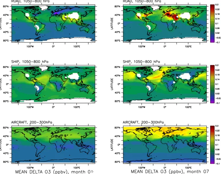
Fig. 5. Mean perturbations of ozone (ppbv) in the lower troposphere (surface-800 hPa) during January (left column) and July (right) for the
different modes of transportation applying a 5% emission reduction. The values for aircraft are shown for 300–200 hPa.
mixing within one model differs less, although horizontally displaced.
4.3 Effects by transport modes
The effects of the emissions from road, ship and aircraft on ozone are shown in Figs. 5–6 for January and July, re-spectively. The results indicate that the road emissions have the strongest effect on ozone in the summer boundary layer over the eastern US and central Europe extending over the Mediterranean to the Arabian Peninsula (Fig. 5). During winter the average effect of road traffic on ozone in the highly industrialized regions of the extratropics almost vanishes or even changes sign, i.e. an increase of road emissions leads to a decrease of ozone during winter. Often under stable bound-ary layer conditions the emissions accumulate, on average to more than 2 ppbv over the industrialized centers over the
eastern US, Europe and parts of East Asia (not shown). Un-der these conditions additional NOx from (road) traffic lo-cally leads to the titration of ozone. In addition the ozone production efficiency can be increased by reduced NOx emis-sions under high NOx conditions leading to a higher ozone productivity per emitted NOx.
Matthes et al. (2007) and Niemeier et al. (2006) find larger relative ozone perturbations due to road traffic of about 10% for some regions in the northern hemisphere boundary layer performing similar model simulations. Part of the deviations to our results can be explained by the use of different emis-sions, which are based on the EDGAR 1990 fuel estimates in Matthes et al. (2007) and are about 25% higher for NOx from road than in this study. The inverted sensitivity of ozone to road emissions during winter is also reported by Niemeier et al. (2006) with the maximum effect over Europe exceeding 25% at the surface. The latter effect is simulated by all five models in our study, which contribute to the average shown
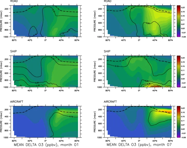
Fig. 6. Same as Fig. 5, but for the zonal mean ozone perturbation. Solid contours show the change relative to the base case simulation,
dashed line indicates the tropopause.
in Fig. 5. Quantitatively, the results of Niemeier et al. (2006) also exceed our calculations by a factor of 2–3 at the surface when scaling our results to 100%. However, since Niemeier et al. (2006) removed the road traffic emissions completely their larger response of ozone is not inconsistent with our results.
Ship emissions have a significant impact throughout the year also with a maximum in July over the central At-lantic/western European region. In the northern hemisphere their effect dominates the boundary layer perturbation dur-ing January and July. Over the northern Pacific region mainly the emission from ships contributes significantly to the ozone perturbation, whereas the North Atlantic region additionally is affected by road emissions, which are transported effi-ciently from the highly polluted Eastern US to the Atlantic.
Not too surprising, in the northern UTLS region (up-per troposphere / lower stratosphere) the effect of aircraft
emissions dominates the ozone perturbation (Fig. 6) being approximately half as large during January compared to July associated with the enhanced level of photochemistry. The ozone perturbation from road traffic during summer is even higher than the perturbation due to aircraft emissions in win-ter, highlighting the role of road traffic for the chemical state of the UTLS in summer (see also Fig. 7). Ship emissions, despite of the high importance in the July boundary layer (Fig. 5) do not show a similar effect in the UTLS, indicat-ing that convective and large scale transport from the marine boundary layer do not have the same impact as continental convection for road traffic.
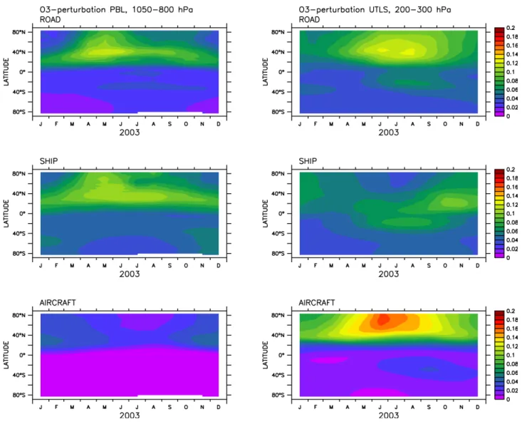
This is also evident from Fig. 7, which shows the tem-poral evolution of the ozone perturbations for the different modes of transport. Comparing ship and road induced ozone perturbations ship emissions have a larger impact on bound-ary layer ozone than road traffic over the whole year. In the
Fig. 7. Temporal evolution of the zonal mean ozone perturbation in ppbv (based on 5% traffic emission change) for the lower troposphere
(left column) and the UTLS region (right).
upper troposphere and lower stratosphere the ozone perturba-tion from road traffic peaks in summer over in the northern mid latitudes exceeding the effect on the boundary layer. The effect of ship emissions does not exhibit this strong seasonal signal in the upper troposphere although their effect on sur-face ozone shows a similar zonal and temporal distribution as for road.
Globally the effect of ship emissions on ozone in the boundary layer is larger than those from road emissions, whereas both are almost equal in the upper troposphere (Ta-ble 5). Notably in the upper troposphere aircraft emissions do not dominate the annual mean global effect between 200– 300 hPa. Their influence is rather concentrated to latitudes poleward of 30◦N (see Fig. 6) whereas road and ship traffic affect the UT globally. Therefore Table 5 also lists the ozone perturbations for the latitude band 30◦–60◦N. In the north-ern upper troposphere aircraft emissions on average account for 1.63% (scaled) to the ozone changes between 30◦–60◦N
with maximum ozone perturbations of 4.2% (scaled). These values are lower than reported by Schumann (1997) and slightly less than in Gauss et al. (2006). A possible rea-son for the discrepancies are the different model resolu-tions since in those studies the applied resoluresolu-tions coarser than 3.75◦×3.75◦ (Schumann, 1998) or T21 (Gauss et al.,
2006). The model with the lowest resolution (p-TOMCAT) in our study also calculates the strongest average perturba-tions which are in the range of 150–232.5 pptv (or 1.6–4.2% when scaling to 100%) with maxima during summer exceed-ing 300 pptv. The coarse resolution leads to an instantaneous spread of the emissions over large areas and volumes which artificially dilutes the NOx and increases the ozone response. Despite the lower model resolution, Kentarchos and Roelofs (2002) obtained similar results as in our study, but they used 15% lower emissions, which could further indicate that a low resolution tends to yield stronger perturbations.
Table 5. Globally averaged ozone perturbations (unscaled) by transport mode for the lower and upper troposphere in pptv. Also given is the
maximum percentage change relative to the unperturbed case. Scaled percentage values are give in italics. The analysis is also shown for the latitude band of 30◦–60◦N indicating zonal mean as well as maximum perturbations (note that the relative and absolute perturbations can occur at different locations resulting in different orders between the transportation sectors).
global 1000–800 hPa 300–200 hPa
MEAN σ % scaled MEAN σ % scaled
ROAD −43.5 11.0 −0.14 −2.89 −58.5 15.0 −0.047 −0.95 SHIP −60.0 13.0 −0.20 −3.99 −56.0 10.5 −0.045 −0.91 AIR −15.0 3.5 −0.05 −1.0 −44.5 23.0 −0.036 −0.72 ALL −118.5 22.0 −0.39 −7.9 −160. 28.5 −0.13 −2.61 30◦–60◦N 1000–800 hPa 300–200 hPa ROAD, mean −77 20 −0.18 −3.66 −89.5 21.0 −0.075 −1.5 SHIP, mean −83.5 18 −0.22 −4.47 −61.0 11.5 −0.05 −1.0 AIR, mean −32 9 −0.08 −1.63 −108. 45.0 −0.08 −1.63 ROAD, max −334.5 – −0.57 −11.41 −172. – −0.21 −4.23 SHIP, max −265.5 – −0.95 −18.9 −136. – −0.28 −5.51 AIR, max −69.0 – −0.15 −3.06 −184.5 – −0.22 −4.31
In addition, plume processes are not captured at all in the models, which may lead to additional uncertainties. Modifi-cations of the emissions through e.g. heterogeneous chem-istry on contrails may lead to enhanced ozone destruction (Meilinger et al., 2005). The recently published update of the reaction of NO with HO2(Cariolle et al., 2008) would lead to a stronger conversion of NOx to HNO3 removing more aircraft-NOxfrom the active phase. On the other hand HNO3 acts as a reservoir species particularly in the lower strato-sphere, which could compensate for this effect. Lightning NOxis unlikely to have caused the differences since there is no systematic difference between the 5 TgN/yr in our study and previous investigations.
Our findings are also evident in the vertical zonal mean cross sections (Fig. 6), highlighting the importance of sur-face emissions from ship and road traffic for the tropical up-per troposphere. It also shows that the impact of road traf-fic is of larger importance for the extratropical troposphere in the northern summer hemisphere (see also Table 5). In the tropics ship emissions are the strongest contributor to the ozone perturbation in the tropical transition layer (TTL), be-ing of greater importance than aircraft emissions there. As evident from Fig. 6 the impact of road and ship emissions seems to influence the whole TTL region from 20◦S–20◦N in particular during northern summer. During January, when the Inter Tropical Convergence Zone (ITCZ) is located in the southern hemisphere, where the emissions are much lower, the TTL is only weakly affected. Note also that for the up-per troposphere in the southern hemisphere the effect of ship emissions is among all modes of transport the strongest con-tributor in January as well as in July (comp. also Fig. 7).
4.4 Relative importance of traffic sectors
In addition to the perturbation of O3the contribution of each individual transport sector relative to the total effect from traffic is of interest. As shown in Fig. 8 the relative impact of road and ship emissions differ substantialy although both are released at the surface. In the region between the sur-face and 900 hPa the relative effect of ship emissions clearly dominates the total perturbations by all traffic emissions in each summer hemisphere. In the southern hemisphere during January the perturbations of ship emissions can almost con-tribute up to 85% of the total ozone perturbation, since ship emissions are the major source of pollutants south of 40◦S. In the northern extratropics the effects from ships are most important in the boundary layer below 950 hPa, where the mean perturbation relative to the background can be as high as 16% (see also Fig. 8). As evident from Fig. 8 the contri-bution of ship emissions is particularly important in the sub-tropical monsoon regions and the tropics, where convection leads to upward transport of the emissions and to a relative contribution of 50% up to the tropical tropopause.
The relative contribution of road emissions peaks in the free troposphere in both summer hemispheres with a pro-nounced seasonal cycle in the northern extratropics. The maximum effect on ozone occurs in July, when convection at these latitudes is strongest. Thus during that time of the year pollutants from road traffic have a much higher proba-bility to be transported to tropopause altitudes compared to winter. This is also evident from Fig. 6 where the ozone per-turbations in July below the tropopause are almost equal to the effect from aircraft.
Note that ship emissions only weakly affect the free and upper troposphere of the northern extratropics during July.
Fig. 8. Relative contribution of each transport sector to the total ozone changes due to the sum of emissions in all transport sectors for
January (left) and July(right).
Since ships largely emit over the open oceans where con-vection is not as strong as over the continents, they have a much lower potential to reach the upper troposphere of the extratropics compared to road emissions. Therefore, in the winter hemispheres the effects of road and ship traffic on ozone show similar patterns (Fig. 6). As indicated by Fig. 8 the relative contribution of road traffic on the free and up-per extratropical troposphere is about 15% larger than that of ships. Directly at the tropopause and in the lower strato-sphere the contribution of aircraft dominates in the northern hemisphere, whereas in the southern hemisphere upper tro-posphere its effect on ozone is the smallest of the three types of traffic.
Note also that the relative contributions as given in Fig. 8 are based on the small emission perturbation and therefore the relative fractions of each sector are different from the
Table 6. Global annual average ozone burden change per an-nual integrated NOx-emission of each respective transport sector in molecules(1O3)/molecules(NOx-emission)
TM4 OSLO LMDz UCI p-TOM mean σ
ROAD 0.31 0.44 0.34 0.35 0.26 0.33 0.05 SHIP 0.47 0.65 0.46 0.57 0.57 0.54 0.07 AIR 1.32 1.22 1.45 1.39 2.78 1.63 0.58
entire removal of each emission source. However, the sen-sitivities as calculated here are expected to be more realistic in view of actual emission changes based on mitigation poli-cies than a total decline of the sources.
Fig. 9. Zonal mean OH perturbation for January (left) and July for a 5% perturbation of road (top), ship (middle) and aircraft (bottom)
emissions, respectively (shading). Contours show the perturbation relative to the base case simulation.
To estimate the efficiency of the ozone perturbation from each transport sector we normalised the additional annual mean ozone burden of each sector to the respective number of NOx molecules emitted. As evident from Table 6 road and ship emissions have similar efficiencies to perturb ozone. However, the NOxemissions from air traffic are almost three times as efficient in producing ozone as those from ships. Since these emissions take place in the UTLS region the life-time of the reservoir species HNO3and PAN are much longer than at the surface. Therefore each NOxmolecule can be re-cycled more often to produce ozone before being removed via precipitation scavenging and dry deposition of HNO3.
Note that despite some individual differences, all models indicate the largest efficiency to perturb ozone for NOx emis-sions from aircraft and the weakest efficiency for road traf-fic. Ship emissions occur largely in remote areas with much lower background pollution compared to road emissions. In
these remote marine regions ozone is more sensitive to NOx -perturbations compared to the polluted land regions, where most of the road emissions are released.
5 OH
5.1 Global OH
The effects of different transport systems on tropopspheric OH concentrations are shown in Fig. 9 for January and July, respectively. Interestingly, ship emissions have the largest impact on the global OH budget in the boundary layer. During northern summer the effect of NOxfrom mar-itime traffic on OH can be as large as 2.5·104molecules/cm3 at 40◦N equivalent to an increase of up to 0.8% (or 5·105 molecules/cm3and 15%,respecively, when scaling to 100%). During winter the effect of ship emissions is about a
Fig. 10. Mean OH perturbation (5% traffic emission reduction) in the boundary layer during January (left) and July (right) between
800-1000 hPa for road- (top) and ship emissions (middle). The effect of aircraft emissions is displayed for 200–300 hPa (bottom).
factor of two lower, thereby reaching a maximum in the lati-tude band from 40◦S to 30◦N. Since the OH concentrations are globally highest in these regions, a (scaled) increase by about 5·105molecules/cm3is of similar magnitude as the an-nual mean concentration in temperate and high latitudes, and is therefore highly significant on a global scale. Also in win-ter the boundary layer OH perturbation is still of the order of 10%. As can be seen from Fig. 9 ship emissions are dominat-ing the annual zonal mean OH perturbation in the boundary layer throughout the year.
The effect of road emissions on the OH distribution shows a pronounced seasonal cycle in particular in the northern hemisphere. The maximum effect occurs during northern summer in the continental boundary layer between 800– 900 hPa reaching 5·103 molecules/cm3 or about 0.18% (zonal annual mean). Since road emissions are largely emit-ted in polluemit-ted industrialized regions over the continents the
zonal mean effect on OH at 1000 hPa is less pronounced than at 900 hPa. High NOx-levels make OH less sensitive to per-turbations as further explained below. However, in particular during northern summer road transport seems to be most im-portant for the lower troposphere in the extratropics up to 500 hPa.
The horizontal distribution (Fig. 10) reveals that the effect on a regional basis can be much stronger than 5·103molecules/cm3. The largest impact is found in the in-dustrialized regions of the Eastern US, central Europe and East Asia reaching 2.5·104molecules/cm3. In these regions OH has the highest potential to be recycled via the reaction of NO with HO2, which is produced after the initial reaction of OH on the carbon containing reactive species (e.g. CO, CH4, NMHCs). The additional NO2 from this reaction in turn leads to the enhanced formation of ozone and OH pro-duction via O1(D). During winter the emissions of CO and
Table 7. Methane lifetime in years for the BASE case and relative changes due to a decrease of traffic emissions of 5%. Scaled mean values
are given in italics. Top boundary for the integration was 50 hPa. Note that no feedback factor is included.
TM4 OSLO LMDz UCI TOMCAT mean σ scaled σ
BASE (yr) 7.23 8.49 10.23 7.45 11.43 8.97 1.63 8.97 1.63
ROAD (%) 0.093 0.068 0.096 0.064 0.081 0.805 0.013 1.61 0.25
SHIP (%) 0.162 0.185 0.206 0.176 0.320 0.206 0.05 4.12 1.02
AIR (%) 0.041 0.032 0.053 0.047 0.09 0.052 0.02 1.04 0.40
NMHCs in these regions act as a direct sink, since solar ra-diation is reduced.
Comparing the impact of road and ship traffic, both sur-face sources of air pollution, the effects on OH are very dif-ferent, although the annual amount of emitted NOxis similar (see Table 1). The zonal mean perturbation of road emis-sions peaks at about 0.2% during northern summer and 0.1% in the southern hemisphere summer. The regional effect dur-ing July can exceed 0.5% in the continental boundary layer for road traffic. As evident from Fig. 9 ship emissions have a larger effect even in the zonal mean. The large differences of both means of transportation on OH can be related to the different regions and pollution conditions. As will be seen later, the sensitivity of OH to traffic emissions is largest in the still relatively pristine regions over the (sub-)tropical oceans. Background concentrations of ozone, NOxand other NMHCs are low, and the solar irradiation and water vapor available for OH formation are high. The recycling potential of OH by NOxis lower than over the continents and is effi-ciently enhanced by ship emissions. The reason is that at al-ready enhanced NOxlevels the reaction of OH with NO2 be-comes a significant sink of hydroxyl radicals, which is not the case in the NOx-poor marine boundary layer. On the other hand these low NOxconcentrations accompanied with high OH make the system more sensitive for NOxperturbations than in polluted areas (Lelieveld et al., 2002). Furthermore, road emissions occur at higher altitudes and latitudes where average water vapor concentrations and solar irradiation are lower and in regions where other anthropogenic sources of pollution cause enhanced NOx levels. The combination of these factors leads to a lower sensitivity of OH to perturba-tions from road traffic than for ship emissions.
The regional perturbation pattern (Fig. 10) illustrates that locally the effects of road and ship emissions on OH are simi-lar during northern summer. The strongest effect is simulated for the ship emissions over the northern subtropical Atlantic in the same region where also ozone exhibits the largest per-turbation (see Fig. 5). Note furthermore that in particular during northern summer the effect on OH at high northern latitudes over Europe is as high as over the eastern subtrop-ical Pacific. Thus the increasing ship traffic at high northern latitudes as a response to the diminishing ice coverage due to the relatively rapid climate change (Lemke et al., 2007, IPCC) might have strong effects on the oxidation capacity
and enhance surface ozone in the Arctic summer by a factor of 2–3 (Granier et al., 2006).
Similar to ozone, aircraft emissions have the largest effect on OH in the upper troposphere of the northern extratropics during summer. Despite the fact that the absolute perturba-tion is about a factor of 2 lower during winter, the relative perturbation exceeds 0.6% (or 12% scaled). The larger rela-tive change during northern winter is due to the strong sea-sonal variation of the background latitudinal OH distribution. During winter the extratropical zonal mean OH at 300 hPa is less than 5·103molecules/cm3, whereas in summer the mean OH in the same region is reaching 1.3·104molecules/cm3.
Note that aircraft emissions have the maximum impact on OH over the subtropical Atlantic south of the main North At-lantic flight corridor. Larger humidity values and the smaller solar zenith angles at lower latitudes during that time of the year are more favourable for OH production than further north. Notice that ship emissions also significantly contribute to the OH perturbation in the middle to upper troposphere of the subtropics up to 200 hPa caused by convective uplift of NOxfrom maritime transport in the tropical and subtropical latitudes.
5.2 Methane lifetime
As seen in the previous section ship emissions have the largest effect on OH leading to the largest reduction of methane lifetime (Table 7) among the three major modes of transport. Methane lifetimes were calculated offline us-ing the monthly mean CH4and OH-fields from each model. Note that no feedback factor is applied here, which would account for long-term equlibration to the new steady-state value as described in Fuglestvedt et al. (1999).
Note further that our results are deduced from a small scale perturbation and that OH is unlikely to respond linearly to a NOxperturbation. We report here on the scaled values since the radiative forcing calculations were performed using the full scale perturbations to allow a robust signal to be obtained (see below). Based on our results road emissions are only half as efficient in perturbing OH on a global scale, and the effects of air traffic are the smallest. The changes by 4.12% (ensemble mean) due to ship emissions exceed the 1.56% re-ported by Eyring et al. (2007), but are close to Fuglestvedt et al. (2008), who reported 5.2%. The NOx emissions in
Fig. 11. Correlations between 1OH and 1NOxfor road traffic (upper row) and ship traffic (lower row) for January (left) and July (right). All coloured points are for low NOxconditions coded by latitudes: (sub-)tropics (red), northern hemisphere (blue > 30◦N) and southern hemisphere (green, < 30◦S). The effect of ship emissions is shown at 950 hPa over the oceans and of road emissions over land up to 850 hPa.
Eyring et al. (2007) of 3.1 TgN/yr are lower compared to the 4.4 TgN/yr in this study (see Table 1) and also in Fuglestvedt et al. (2008), but it is unlikely that this alone has caused the large differences. In addition the emission patterns of both ship emission data sets are very different. The distribution of the ship emissions in Eyring et al. (2007) and Stevenson et al. (2006) is based on the EDGAR3.2 dataset, where the emis-sions are mainly concentrated on the major shipping routes. The ship emissions used in QUANTIFY have been gener-ated by merging the daily fields of COADS and AMVER data (Automated Mutual-assistance Vessel Rescue system) (Endresen et al., 2003) and are distributed over a larger area (comp. Fig. 1 and Eyring et al. (2007), their Fig. 1). This explains the stronger effect on CH4lifetime, since a larger fraction of NOx is emitted over the tropical oceans over a widespread area. Recall that conditions for OH production are favourable at low latitudes and in addition the local CH4 lifetime by OH oxidation is shortest also due to the high tem-peratures.
Both factors are also the reason for the smaller effects of road and aircraft emissions on OH and on the methane lifetime, since they occur in higher latitudes and altitudes where annual mean OH concentrations and temperatures are lower.
5.3 Sensitivity of OH production
From Fig. 10 it is evident that ship emissions strongly affect the still relatively clean regions mostly in the tropics, but also in the extratropics. In contrast, road emissions are largely released into an environment already affected by emissions from other sources both of natural (soils, lightning) and an-thropogenic origin. The different effects on OH from road and ship traffic in the boundary layer are presented in Fig. 11 showing the 1NOxand 1OH perturbations for road and ship emissions, respectively. Coloured data points are indicative for low NOx conditions (< 20 pptv) in different latitude belts. The correlations show that the sensitivity of OH to NOx perturbations is much higher for ship traffic than for road emissions even under low-NOxconditions. As expected the 1OH/1 NOx-ratio is highest for ship emissions in the relatively pristine maritime conditions in the tropics (red). The impact of road emissions is insignificant in these regions under low-NOxconditions. In particular in the southern ex-tratropics (green dots) there is a high sensitivity to NOx per-turbations from ships.
In relatively NOxenriched conditions, under which most of the road emissions occur, the effect of ship NOx on OH is also higher than that of road traffic. The OH response
Table 8. Radiative forcings from changes in ozone, changes in methane and methane-induced ozone change by model and transportation
sector in mW/m2. Note that the fully scaled perturbations were used to calculate the forcings
ROAD SHIP AIRCRAFT
O3 CH4 O3(CH4) total O3 CH4 O3(CH4) total O3 CH4 O3(CH4) total TM4 26.3 −16.8 −7.0 2.5 23.8 −29.3 −12.3 −17.8 12.7 −7.3 −3.1 2.3 OSLO 32.7 −12.3 −5.1 15.3 30.0 −32.7 −13.7 −16.5 10.8 −5.7 −2.4 2.8 LMDz 32.8 −17.2 −7.2 8.4 26.1 −37.1 −15.6 −26.6 14.4 −9.6 −4.0 0.8 UCI 28.3 −11.5 −4.8 11.9 29.4 −31.6 −13.3 −15.6 13.2 −8.4 −3.5 1.3 TOMCAT 19.2 −14.7 −6.2 −1.7 27.24 −55.0 −23.1 −50.8 30.2 −16.1 −6.8 7.3 mean 27.9 −14.5 −6.1 7.3 27.3 −37.2 −15.6 −25.5 16.3 −9.4 −4.0 2.9 σ 5.0 2.3 1.0 6.2 2.2 9.3 3.9 13.3 7.1 3.6 1.5 2.3
for ship emissions is an almost linear function at the lower 1NOxlevels, whereas the efficiency of OH production from road is weaker and levels off at lower 1NOx perturbations. OH perturbations from road NOx emissions maximize at 2·104molecules/cm3, while OH perturbations from ship ex-ceed 2.5·104molecules/cm3and show no saturation tendency. This can be attributed to the higher level of NMHCs and NO2 over the continents acting as a sink for OH at high pollution levels.
5.4 Radiative forcings
We briefly report the radiative forcings resulting from the transport-induced ozone changes using the mean perturba-tions scaled to 100% to obtain a robust signal. The ozone ra-diative forcing (cloudy skies including stratosphere tempera-ture adjustment) was calculated using the University of Oslo radiative transfer code (e.g. Myhre et al., 2000). The forcing was calculated using the 3-D monthly mean ozone pertur-bation fields generated by each of the participating models. The annual and global-mean forcings are shown in Table 8. Averaged over the models, the road and shipping induced forcings are about the same (27 mWm−2) with aviation con-tributing around 16 mWm−2. However this hides significant intermodel differences. For three models, the road forcing is highest, followed by shipping followed by aviation. For p-TOMCAT this order of importance is reversed.
The forcings are within their stated uncertainties in broad agreement with those reported by Fuglestvedt et al. (2008) except for road traffic, for which a value of 54±11 mWm−2 was reported. A main reason for the weaker radiative forc-ing is the use of lower road emissions in this study com-pared to Fuglestvedt et al. (2008). Note further that we use a small perturbation approach. As shown in Sect. 2.1 the ozone response to a perturbation of road traffic emissions is smaller compared to a total decline of the road emission source. Thus, the ozone burden change and the associated radiative forcing are likely to be smaller.
Table 8 also shows simple estimates for two further forc-ings which result from the emissions and the consequent
ozone and OH changes – the change in methane and the re-sulting change in ozone. These estimates are derived follow-ing the method given in Berntsen et al. (2005). First, the change in methane is calculated from the scaled percentage change in lifetime given in Table 7, multiplied by a feedback factor of 1.4 to account for the impact of methane changes on its own lifetime. The radiative forcing is then calculated as-suming a methane specific forcing of 0.37 mWm−2ppbv−1, which is a linearization of the IPCC (2001) forcing for a background methane mixing ratio of 1740 ppbv and a ni-trous oxide mixing ratio of 319 ppbv. Second, the radia-tive forcing due to the methane-induced ozone change (see Eq. B6 of Berntsen et al. (2005)) is estimated using multi-model means of both the response of ozone to a methane change (a 10% increase in methane leads to a 0.64 DU in-crease in ozone) and an ozone specific radiative forcing of 42 mWm−2DU−1from IPCC (2001). Together these lead to a methane-induced ozone radiative forcing which is 0.42 times the methane radiative forcing. This method assumes that the methane change is in equilibrium with the change in OH, which will require several decades of constant emissions to achieve.
The mean “net” forcing from the three components (Ta-ble 8) is positive for road and aviation and negative for ship-ping, as also found by Fuglestvedt et al. (2008). However, the residual nature of this net forcing leads to large inter-model differences, particularly for road and air where the standard deviation is almost as large as the mean. For air-craft emissions the effect on ozone and methane as calculated for the individual models is on average somewhat weaker as in Sausen et al. (2005), which can partly be attributed to the small perturbation approach, but also to the higher model res-olution used here (Rogers et al., 2002).
All models simulate much stronger forcings for ship emis-sions compared to Eyring et al. (2007) which is most likely due to the very different distribution of the emissions, but also due to lower emission estimates of NOx as stated in the previous section. Fuglestvedt et al. (2008) obtain forc-ings of 32±9 mWm−2for ozone and −43±13 mWm−2for methane, which both cover the range of our individual model