Decadal trends in global CO emissions as seen by MOPITT

HAL Id: hal-01805229

https://hal.archives-ouvertes.fr/hal-01805229

Submitted on 8 Oct 2020

HAL is a multi-disciplinary open access

archive for the deposit and dissemination of

sci-entific research documents, whether they are

pub-lished or not. The documents may come from

teaching and research institutions in France or

abroad, or from public or private research centers.

L’archive ouverte pluridisciplinaire HAL, est

destinée au dépôt et à la diffusion de documents

scientifiques de niveau recherche, publiés ou non,

émanant des établissements d’enseignement et de

recherche français ou étrangers, des laboratoires

publics ou privés.

MOPITT

Y. Yin, F. Chevallier, P. Ciais, G. Broquet, A. Fortems-Cheiney, I. Pison, M.

Saunois

To cite this version:

Y. Yin, F. Chevallier, P. Ciais, G. Broquet, A. Fortems-Cheiney, et al.. Decadal trends in global CO

emissions as seen by MOPITT. Atmospheric Chemistry and Physics, European Geosciences Union,

2015, 15 (23), pp.13433-13451. �10.5194/acp-15-13433-2015�. �hal-01805229�

www.atmos-chem-phys.net/15/13433/2015/ doi:10.5194/acp-15-13433-2015

© Author(s) 2015. CC Attribution 3.0 License.

Decadal trends in global CO emissions as seen by MOPITT

Y. Yin1, F. Chevallier1, P. Ciais1, G. Broquet1, A. Fortems-Cheiney2, I. Pison1, and M. Saunois1

1_{Laboratoire des Sciences du Climat et de l’Environnement, CEA-CNRS-UVSQ, UMR8212, Gif-sur-Yvette, France}

2_{Laboratoire Interuniversitaire des Systèmes Atmosphériques, CNRS/INSU, UMR7583, Université Paris-Est Créteil et} Université Paris Diderot, Institut Pierre Simon Laplace, Créteil, France

Correspondence to: Y. Yin (yi.yin@lsce.ipsl.fr)

Received: 20 April 2015 – Published in Atmos. Chem. Phys. Discuss.: 22 May 2015 Revised: 28 October 2015 – Accepted: 17 November 2015 – Published: 7 December 2015

Abstract. Negative trends of carbon monoxide (CO) concen-trations are observed in the recent decade by both surface measurements and satellite retrievals over many regions of the globe, but they are not well explained by current emis-sion inventories. Here, we analyse the observed CO concen-tration decline with an atmospheric inversion that simultane-ously optimizes the two main CO sources (surface emissions and atmospheric hydrocarbon oxidations) and the main CO sink (atmospheric hydroxyl radical OH oxidation). Satellite CO column retrievals from Measurements of Pollution in the Troposphere (MOPITT), version 6, and surface observations of methane and methyl chloroform mole fractions are assim-ilated jointly for the period covering 2002–2011. Compared to the model simulation prescribed with prior emission in-ventories, trends in the optimized CO concentrations show better agreement with that of independent surface in situ measurements. At the global scale, the atmospheric inversion primarily interprets the CO concentration decline as a de-crease in the CO emissions (−2.3 % yr−1), more than twice the negative trend estimated by the prior emission invento-ries (−1.0 % yr−1). The spatial distribution of the inferred decrease in CO emissions indicates contributions from west-ern Europe (−4.0 % yr−1), the United States (−4.6 % yr−1) and East Asia (−1.2 % yr−1), where anthropogenic fuel com-bustion generally dominates the overall CO emissions, and also from Australia (−5.3 % yr−1), the Indo-China Peninsula (−5.6 % yr−1_{), Indonesia (−6.7 % yr}−1_{), and South America} (−3 % yr−1_{), where CO emissions are mostly due to biomass} burning. In contradiction with the bottom-up inventories that report an increase of 2 % yr−1 over China during the study period, a significant emission decrease of 1.1 % yr−1 is in-ferred by the inversion. A large decrease in CO emission factors due to technology improvements would outweigh the

increase in carbon fuel combustions and may explain this de-crease. Independent satellite formaldehyde (CH2O) column retrievals confirm the absence of large-scale trends in the at-mospheric source of CO. However, it should be noted that the CH2O retrievals are not assimilated and OH concentrations are optimized at a very large scale in this study.

1 Introduction

Carbon monoxide (CO) is an air pollutant that leads to the formation of tropospheric ozone (O3) and carbon dioxide (CO2). It is the major sink of the tropospheric oxidant hy-droxyl radical (OH), and hence influences concentrations of methane (CH4)and non-methane volatile organic com-pounds (NMVOCs) (Logan et al., 1981). It contributes to an indirect positive radiative forcing of 0.23 ± 0.07 W m−2 at the global scale (IPCC, 2013). Atmospheric CO has two main sources: (i) direct surface CO emissions from fuel combustion and biomass burning, estimated to be ∼ 500– 600 TgCO yr−1and ∼ 300–600 TgCO yr−1, respectively, by emission inventories (Granier et al., 2011, and references herein), and (ii) secondary chemical oxidation of hydrocar-bons in the troposphere, estimated to be a source of ∼ 1200– 1650 TgCO yr−1_{with considerable differences among} stud-ies (Holloway et al., 2000; Pétron et al., 2004; Shindell et al., 2006; Duncan and Logan, 2008). The sink of CO is mainly through oxidation by OH (Logan et al., 1981), which defines an average lifetime of 2 months for CO in the atmosphere.

Surface in situ measurements in Europe (Zellweger et al., 2009; Angelbratt et al., 2011), over the USA (Novelli et al., 2003; EPA, 2015), in some large cities in China (Li and Liu, 2011), and in many other places (Yoon and Pozzer,

2014), indicate that CO concentrations have been decreas-ing for more than 10 years. Negative trends have also been observed by various satellite sensors (MOPITT; the Tropo-spheric Emission Spectrometer – TES; and the AtmoTropo-spheric Infrared Sounder – AIRS) over most of the world (Warner et al., 2013; Worden et al., 2013). In particular, strong CO con-centration decreases are seen from these satellite retrievals over eastern China and India (Worden et al., 2013), where bottom-up inventories report increasing emissions (Granier et al., 2011; Kurokawa et al., 2013).

Atmospheric chemistry transport models (ACTMs) pre-scribed with emission inventories are commonly used to analyse the role of emissions in the atmospheric concentra-tion. Most of these simulations tend to underestimate CO concentrations in the middle to high latitudes of the North-ern Hemisphere (NH), whereas they overestimate them over emission hotspots (Shindell et al., 2006; Duncan et al., 2007; Naik et al., 2013; Stein et al., 2014; Yoon and Pozzer, 2014). This bias reveals an incorrect balance between CO sources, at the surface and in the atmosphere, and CO sinks (Naik et al., 2013). Understanding this model–data misfit is challeng-ing because surface emissions and chemical production each account for about half of the total CO sources, and because the sink term removes an amount of CO equivalent to all the sources within a few weeks. Changes in each source and sink term could have contributed to the observed CO concentra-tion decrease, even though only CO emission trends are usu-ally discussed (Khalil and Rasmussen, 1988; Novelli et al., 2003; Duncan and Logan, 2008).

In principle, the attribution of the mean balance between sources and sinks and of their trends can be made with Bayesian inversion systems that infer the CO budget terms based on (i) measurements of CO and species related to the CO sources and sinks, (ii) some prior information about the budget terms and spatial distributions, (iii) a CTM model to link emissions and chemistry to concentrations, and (iv) a description of the uncertainty in each piece of information. Various inversion studies have estimated regional or global CO budgets using CO surface observations (Bergamaschi et al., 2000; Pétron, 2002; Butler et al., 2005) or satellite re-trievals (Arellano et al., 2004; Pétron et al., 2004; Stavrakou and Müller, 2006; Chevallier et al., 2009; Fortems-Cheiney et al., 2009, 2011, 2012; Kopacz et al., 2010; Hooghiem-stra et al., 2012; Jiang et al., 2013). Here, we use the Python Variational – Simplified Atmospheric Chemistry (PYVAR-SACS) inversion system of Pison et al. (2009), Chevallier et al. (2009) and Fortems-Cheiney et al. (2009, 2011, 2012) to infer the most likely origin of the observed CO concentration decrease over the past decade (2002–2011).

In contrast to most CO inversion systems cited above, which focused on a single species, PYVAR-SACS simulta-neously assimilates observations of the main species in the

chemical oxidation chain of CH4–CH2O–CO and methyl

chloroform (MCF), a species that only reacts with OH and therefore informs about its concentration. The

PYVAR-SACS system optimizes the interconnected sources and sinks of the four species in a statistically and physically consistent way at the model resolution of 3.75◦_×2.5◦_(longitude,

lati-tude) on an 8-day basis, therefore being suitable for address-ing the above-described attribution problem of the CO varia-tions within the limit of the observation information content. The primary data source about CO in this study is MO-PITT, a multi-channel thermal infrared (TIR) and near-infrared (NIR) instrument on board the EOS-Terra satellite (Deeter, 2003). MOPITT provides the longest consistent time series of satellite CO retrievals to date. The algorithm has un-dergone continuous improvements and the archive has been reprocessed several times (Deeter et al., 2013). Most of the above-cited satellite-based inversion studies used version 4 or earlier versions of the MOPITT CO retrievals, in which a noticeable instrumental drift was reported (Deeter et al., 2010). In version 5, this drift has been corrected together with other improvements (Deeter et al., 2013; Worden et al., 2013). Here, we use the further improved version 6 that has no noticeable bias in the trends of the CO total column (Deeter et al., 2014), to attribute the CO concentration de-cline by assimilation in our atmospheric inversion system.

The structure of the paper is as follows. Section 2 describes the inversion system and the data sets. Section 3 presents the inversion results on CO concentrations and associated trends. We show a brief evaluation of the inversion ability to fit the assimilated data and we cross-evaluate the optimized sur-face CO concentrations against independent station measure-ments. Then, we compare the CO concentration trend in the MOPITT retrievals, in the surface measurements, and in cor-responding modelling results before and after the inversion. Section 4 shows the trend analysis of the prior and posterior simulated CH2O and OH concentrations. CH2O concentra-tions are representative of the chemical CO sources and we evaluate the model values against retrievals of its dry air col-umn (XCH2O)made from observations of the Ozone Monitor-ing Instrument (OMI) aboard EOS Aura. OH regulates CO sinks, but is an extremely short-lived compound whose con-centrations are difficult to measure (Mao et al., 2012). Lack-ing direct global observation data, we discuss its uncertain-ties with two contrasting prior OH fields. Section 5 presents the inverted CO budget, including atmospheric burden, emis-sion, chemical production and chemical loss. Section 6 sum-marizes this work, discusses the sources of uncertainties and provides some perspectives for future works.

2 Method and data

2.1 Inversion system

The PYVAR Bayesian inversion system, initially introduced by Chevallier et al. (2005), aims at adjusting a series of target variables (jointly called x), so that they become consistent with both the atmospheric observations (y) and a priori state

!"! !" !!!!!! !" !!"!!"!!"!!!!!!!"# !" ! 1 Surface  obs  

(WDCGG)     MOPITT  v6  TIR&TNR     Surface  obs  (WDCGG)   Observa(on  

State   vector  

Prior   _emission  Surface   Emission   +   oxidaCon   from   NMVOCs   Surface  

emission   emission  Surface  

TransCom/ INCA   (modeled  in  3D)   In iC al  st at e   Scaling   factor   (gridded)   Surface   emission   (gridded)   Surface   emission   (gridded)   Surface   emission   (gridded)   Scaling   factors   (gridded)   Scaling   factor   (for  6  big   regions)  

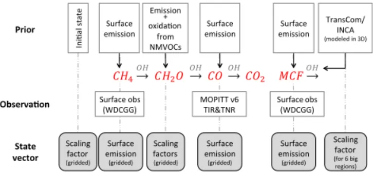
Figure 1. Schematics of the input information provided to the

in-version and of the inin-version state vector.

(xb)given their respective uncertainties, represented by error covariance matrices R and B. By iteratively minimizing the following cost function J , PYVAR finds the optimal solution for x in a statistical sense:

J (x) =1 2(x − x b₎T_B−1_{(x − x}b₎ +1 2(H(x) − y) T_R−1_{(H(x) − y) ,}

where H is the combination of a CTM and of an interpolation operator that includes the combination with the retrieval prior CO profiles and averaging kernels (AKs) for MOPITT.

Our CTM is the general circulation model of Laboratoire de Météorologie Dynamique (LMDz) version 4 (Hourdin et al., 2006), nudged towards winds analysed by the Euro-pean Centre for Medium-Range Weather Forecasts, run in an off-line mode with precomputed atmospheric mass fluxes, and coupled with the SACS chemistry module (Pison et al., 2009). SACS is a simplification of the Interaction with Chemistry and Aerosols (INCA, Hauglustaine, 2004) full chemistry model.

The chemical chain is shown in Fig. 1. It includes surface emissions of CO, CH4, CH2O and MCF. The 3-D contribu-tion of NMVOC oxidacontribu-tion to CH2O production has been pre-calculated by the LMDz-INCA (Folberth et al., 2006). OH links all the species together. Reaction kinetic and photolysis rates, as well as fields of species that are not represented as tracers in PYVAR-SACS (e.g. O1D, O2, Cl), are based on the LMDz-INCA simulation. The initial states are produced by LMDz-INCA. The CTM in PYVAR-SACS has a time step of 15 min for the dynamics (advection) and of 30 min for the physics (convection, boundary layer turbulence) and chem-istry, a horizontal resolution of 3.75◦_×2.5◦_(longitude,

lati-tude), and a vertical resolution of 19 eta-pressure levels from the surface to the top of the atmosphere.

The state vector x contains the following variables as shown in the grey boxes in Fig. 1: (1) grid-point scaling fac-tors for the initial mixing ratios of the four trace gas species (CO, CH4, CH2O, MCF); (2) grid-point 8-day mean surface emissions of CO, CH4, and MCF; (3) grid-point 8-day scal-ing factors to adjust the sum of CH2O surface emissions and

CH2O production from NMVOC oxidation; and (4) 8-day

scaling factors to adjust the column-mean OH concentrations over six big boxes of the atmosphere over the globe: three lat-itudinal boxes (90–30◦_{S, 30}◦_S–0◦_{, 0}◦_–30◦_{N) and three}

lon-gitudinal boxes north of 30◦N (North America: 180–45◦W; Europe: 45◦W–60◦E; Asia: 60–180◦E). The longitudinal di-vision of the band north of 30◦N is an improvement com-pared to previous PYVAR studies, with four latitudinal bands in total to optimize OH. As there are available surface sta-tions with long-term MCF observasta-tions within each of the sub-regions, this allows adjusting of separately continental differences of OH.

2.2 A priori information

Previous configurations of PYVAR-SACS have been de-scribed by Chevallier et al. (2009) and Fortems-Cheiney et al. (2011). We have improved the configuration as described below.

2.2.1 Prior sources and sinks

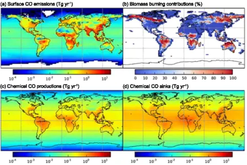
For prior anthropogenic fossil fuel and biofuel CO emissions, we use the monthly MACCity emission inventory of Lamar-que et al. (2010) that arguably underestimates emissions less than other global inventories (Granier et al., 2011; Stein et al., 2014). For biomass burning, we updated the version of Global Fire Emissions (GFED) from version 2 (van der Werf et al., 2006) to version 3.1 (Van der Werf et al., 2010). The latter has various improvements including the definition of different fire types, with specific consideration for defor-estation and peatland fires. We also increased the tempo-ral resolution of biomass burning emissions from monthly to weekly (aggregated from GFEDv3.1 daily emissions, Mu et al., 2011). Additionally, we consider in this study bio-chemical CO emissions from oceans that were neglected before, based on an ocean biogeochemical model simula-tion (Aumont and Bopp, 2006). These monthly ocean CO fluxes add up to a global annual sum of 54 TgCO yr−1 with-out inter-annual variability. We still consider neither biogenic CO emissions over land nor surface CO deposition, because these two terms are relatively small and are of a similar order of magnitude (Duncan et al., 2007). The prior CO emissions are summarized in Table 1 and the distribution of the mean annual prior CO surface emissions is shown in Fig. 2a. The relative contribution of biomass burning is shown in Fig. 2b. The prior CH4and MCF emissions have also been updated compared to Fortems-Cheiney et al. (2012) and are similar to that of Cressot et al. (2014). HCHO production prior fields have been pre-calculated by LMDz-INCA (Folberth et al., 2006), with prescribed NMVOC emission data sets detailed in Fortems-Cheiney et al. (2012). The prior distribution of mean annual CO chemical sources in the troposphere from the oxidation of both CH4and NMVOCs is shown vertically integrated in Fig. 2c.

Table 1. Prior data sets for the sources and sinks of CO. Mean annual sums are calculated for the period from 2002 to 2011. The global

annual prior error budgets are reported and the TransCom-OH field is used. The sum of surface emissions and chemical sources are shown in bold.

Sectors Mean annual Data set/ References

sum (Tg yr−1) model

CO Sources:

Biomass burning 327 GFEDv3.1 Van der Werf et al. (2010)

Anthropogenic emissions 588 MACCity Lamarque et al. (2010)

Ocean 54 PISCES Updated from Aumont et al. (2006)

Sum of surface emissions 969 ± 180a

Oxidation from NMVOC 335 ± 43b LMDz-INCA Folberth et al. (2006)

Oxidation from CH4 885 ± 92c

Sum of chemical sources 1220

Sinks:

Oxidation by OH 2197 TransCom-OH Patra et al. (2011)

a_{The uncertainty represents the SD of the global annual error budgets in the prior CO emissions in the inversion configuration.}b_{The SD is} calculated into the equivalent CO amount from global annual error budgets of the pre-calculated CH₂O production fields.c_{The SD is calculated} into the equivalent CO amount from global annual error budgets of the prior CH₄emissions assuming they are all oxidized into CO in a single step. The prior CH4emission (506 TgCO yr−1)data sets are detailed in Cressot et al. (2014).

Figure 2. Distribution of prior budget terms for CO. Annual mean values per each model grid (2.5 latitude × 3.75 longitude) from 2002

to 2011 are shown. (a) Surface CO emissions, (b) relative percentages of CO emissions from biomass burning over land, (c) atmospheric

CO productions from CH4and NMVOC, and (d) atmospheric CO chemical sinks. The chemical productions and sinks are calculated with

TransCom-OH.

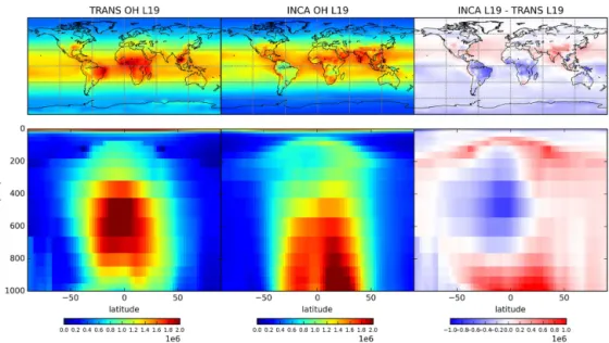
Previous PYVAR-SACS studies used prior OH informa-tion from a multi-year simulainforma-tion by LMDz-INCA (Hauglus-taine, 2004). Here, we use another field that was prepared for the international TransCom-CH4experiment of Patra et al. (2011). The annual mean horizontal and vertical distribu-tion of OH concentradistribu-tions for both OH fields and their dif-ferences are shown in Fig. 3. Compared to the INCA-OH, the TransCom OH has a lower OH concentration in the NH, and a lower concentration over the tropics and the South-ern Hemisphere (SH). Thus, the TransCom-OH has a north– south inter-hemisphere ratio of around 1, whereas the

INCA-OH has a ratio of 1.2. There are also vertical differences be-tween these two OH fields: in general, TransCom-OH has higher OH concentrations in the mid-troposphere over the tropics and in the top layers above 100 hPa, whereas INCA-OH has higher INCA-OH concentrations in the lower troposphere below 700 hPa. The prior distribution of the CO sinks sim-ulated with TransCom-OH is shown vertically integrated in Fig. 2d.

Figure 3. Spatial and vertical distribution of OH concentration in TransCom and INCA and their relative differences. The TransCom OH is

interpolated from its original 60 pressure levels into the LMDz 19 eta-pressure levels.

2.2.2 Prior error statistics

The prior flux uncertainty, defined by the standard devia-tion (SD) of each grid-point 8-day flux, is described below. For CO emission uncertainties, we define the SD for each year based on the maximum value of the emission time se-ries during the corresponding year for each grid point (noted as fmax), in order to account for the uncertainty of the fire timing. Then, to account for (i) the possibility of undetected small fires that can contribute to as much as 35 % of the global biomass burning carbon emissions (Randerson et al., 2012), and (ii) potentially higher CO emission factors during small fires that were not specifically considered in current fire emission inventories (van Leeuwen et al., 2013), we de-fine a fire emission threshold of 1.0 × 10−10kg CO m−2s−1. If the prior emission is less than the threshold (no fire a priori, but there could be one in reality), the SD is set as 100 % of fmax; otherwise (fire a priori, but possibly of a too small magnitude), the SD is set as the maximum value be-tween 1.0 × 10−9kg CO m−2s−1and 50 % of fmax. In such a way, we allow the system to relax the constraint on the prior emission to account for undetected small emissions, but we keep the global uncertainty (∼ 180 TgCO yr−1) consis-tent with current bottom-up inventories (Granier et al., 2011; Van der Werf et al., 2010). For simplicity, this error setting also serves for anthropogenic fuel consumption.

The prior CH4emission uncertainty is defined as 100 % of the maximum value of the prior emissions in the grid cell and its eight neighbours in the corresponding month. The MCF prior emission uncertainty is set at ±10 % of the flux, as its emissions are supposed to be well known. The uncertainty of CH2O production is assumed to be 100 % of its concur-rent prior CH2O production. The uncertainties of initial

con-centration scaling factors are set at 10 % for the four species (CO, CH4, CH2O, MCF). Errors in OH 8-day scaling factors are set at ±10 %.

The spatial error correlations of the a priori are assigned to all variables following Chevallier et al. (2007), defined by an e-folding length of 500 km over the land and 1000 km over the ocean. Temporal error correlations are defined by an e-folding length of 8 weeks for MCF and 2 weeks for the other species including OH. No inter-species flux error correlations are considered.

2.3 Observations for assimilation

2.3.1 Data sets

We assimilate three data streams: (i) MOPITTv6 satellite CO total column retrievals (noted as XCOhereafter) and surface in situ measurements of (ii) CH4and (iii) MCF.

MOPITT retrievals have been available since March 2000, but the instrument experienced a cooler failure from May to August 2001, which artificially changed the retrieval mean level (Deeter et al., 2010). An instrument anomaly also led to a 2-month lack of data in 2009 from the end of July un-til September, without any significant change in the retrieval mean level. For the sake of consistency, given our focus on trends, we select the measurements for the decade from 2002 to 2011, during which both the MOPITT retrievals and the prior emission inventories are homogeneous (GFEDv3.1 has not been publicly updated for the years after 2011).

We use the level 2 “multispectral” near-infrared and ther-mal infrared (NIR/TIR) CO retrievals of MOPITTv6 that offer the best description of CO in the lower troposphere among the MOPITT products (Deeter et al., 2014). The

MO-PITT vertical profiles (prior and retrieved CO profiles and associated AKs) are defined on ten vertical pressure levels. Given the limited vertical resolution of the retrievals and the focus on surface emissions, it has been common practice in previous inversion studies starting from Pétron et al. (2004) to assimilate the 700 hPa pressure level retrievals only, as a good compromise between proximity to the surface and lim-ited noise. However, Deeter et al. (2014) noted that the re-trievals at some individual vertical levels still suffered from small bias drifts, while such drifts were not seen in the re-trieved integrated columns. Furthermore, the interpretation of vertically integrated columns in the inversion is less ham-pered by flaws in CTM vertical mixing and vertical sink dis-tribution than for level retrievals (Rayner and O’Brien, 2001). For these two reasons, we assimilate the column retrievals rather than level retrievals. Night-time observations, observa-tions with a solar zenith angle larger than 70◦_{, with latitudes}

within 25◦_{from the poles, or with surface pressures less than}

900 hPa, are excluded, since they may be of lower quality or more difficult to model (Fortems-Cheiney et al., 2011). We average the 22 × 22 km2 retrievals at the 3.75◦×2.5◦ model resolution within 30 min time steps. The model XCO retrievals are calculated in a consistent way as in the MO-PITT XCOretrievals with their original prior CO profiles and AKs averaged for each model grid.

Surface measurements of CH4 and MCF from various

networks are assimilated together with MOPITT XCO. The data sets are downloaded from the World Data Centre for Greenhouse Gases (WDCGG, http://ds.data.jma.go.jp/gmd/ wdcgg/). Stations that recorded more than 6 years of data without gaps larger than 1 year are included. The list of sta-tions is given in Tables S1 and S2 in the Supplement. For the surface measurements, a data filtering process is conducted in order to remove outliers that the global model may not be able to capture. We exclude (i) observations exceeding 3σ of the de-trended and de-seasonalized daily time series and (ii) observations whose misfit against the prior simula-tion exceeds 3σ of the de-trended and de-seasonalized misfit between observations and forward modelling values.

2.3.2 Observation error statistics

The observation error covariance matrix R is diagonal in order to simplify calculations. Observation errors are com-binations of measurement errors (quantified by the data providers), representativeness errors and CTM errors. For XCO, as we have averaged a large number of observations in each grid box (see Sect. 2.3.1), the representativeness error is effectively much reduced and is not considered specifically. The CTM error is set at 30 % (SD) of the modelled values for XCO. For CH4and MCF, synoptic variability (estimated from the residues of de-trended and de-seasonalized data) is used as a proxy for the CTM and representativeness errors, which largely dominate the observation error. The global mean measurement error for Xco is around 6.4 ± 2.9 ppb, which

is approximately 8.2 ± 1.9 % of the corresponding XCO ob-servations. The measurement errors are set as 3 ppb for CH4 and 1.2 ppt for MCF if not explicitly provided by the surface observation data sets.

2.4 Observations for cross-evaluation

We use two data sets for independent evaluation of the inver-sion results.

The first one is made of CO surface observations archived at the WDCGG. The same site selection and data filtering process as for CH4and MCF surface measurements are ap-plied (see the list of stations in Table S3).

The second evaluation data set gathers CH2O total

columns retrieved from OMI by the Smithsonian Astrophys-ical Observatory (SAO). We use version 3, release 2, of this product (González Abad et al., 2015). Since these data are not available before mid-2004, they do not cover our study period completely: for the sake of consistency, we do not as-similate them (in contrast to Fortems-Cheiney et al., 2012) and we keep them for evaluation. We select observations that are tagged as “good” by the provider’s quality flag, which have a solar zenith angle less than 70◦and a cloud cover be-low 20 %, and are not affected by the “row anomaly”.

2.5 Trend analysis

The long-term trend in this study is estimated by least-square curve fitting of the following function, which includes a constant, a linear component, and seasonal variations repre-sented by four harmonics:

f (t ) = a0+a1t + 4 X

n=1

cn[sin(2nπ t + ϕn)] .

If not particularly specified, all the trends mentioned in this paper refer to a1.

3 CO concentrations and associated trends

3.1 Evaluation of the inversion framework’s ability to

fit the data

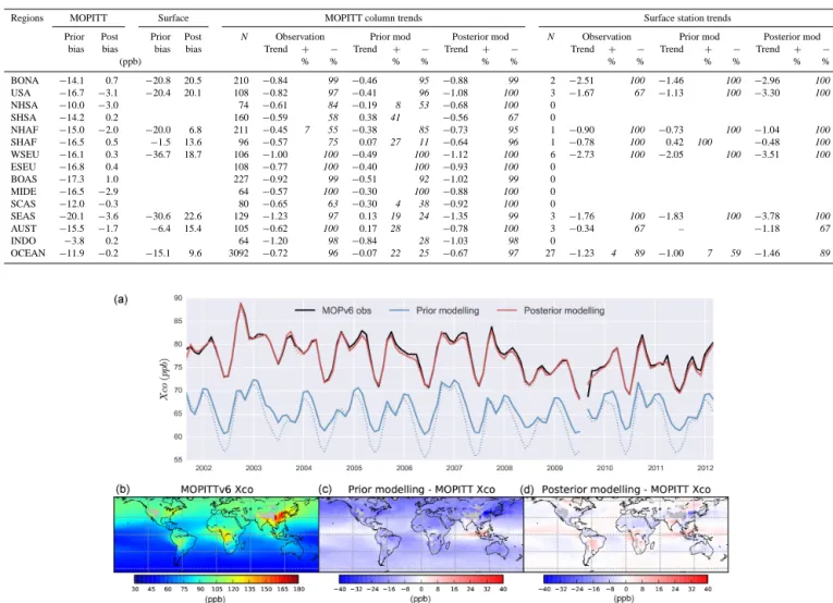
Figure 4a shows the time series of the global mean mole frac-tion of the MOPITT XCO retrievals (black), and the prior (blue) and the posterior (red) XCOretrievals (calculated from model simulations with the MOPITT prior profiles and av-eraging kernels). Compared to the MOPITT XCO, the prior

XCO simulation is on average 15 % lower when modelled

with TransCom-OH and 17 % lower when modelled with INCA-OH. The global mean posterior XCOfits the observa-tion irrespective of the OH field used.

The spatial distribution of the multiyear mean XCO ob-served by MOPITT (2002–2011) shows a latitudinal gradient from north to south, with some high values over East Asia,

Table 2. Summary of CO model–data comparison and trend analysis for MOPITT satellite retrievals, surface station observations and

corresponding prior/posterior modelling. Trends for each region (in the unit of ppb yr−1)are the mean values for all the grids whose trends

are significant at the 95 % confidence level. The percentages of significant trends (shown in italic) are also given per model grid for positive (+) and negative (−) respectively.

Regions MOPITT Surface MOPITT column trends Surface station trends

Prior Post Prior Post N Observation Prior mod Posterior mod N Observation Prior mod Posterior mod bias bias bias bias Trend + − Trend + − Trend + − Trend + − Trend + − Trend + −

(ppb) % % % % % % % % % % % % BONA −14.1 0.7 −20.8 20.5 210 −0.84 99 −0.46 95 −0.88 99 2 −2.51 100 −1.46 100 −2.96 100 USA −16.7 −3.1 −20.4 20.1 108 −0.82 97 −0.41 96 −1.08 100 3 −1.67 67 −1.13 100 −3.30 100 NHSA −10.0 −3.0 74 −0.61 84 −0.19 8 53 −0.68 100 0 SHSA −14.2 0.2 160 −0.59 58 0.38 41 −0.56 67 0 NHAF −15.0 −2.0 −20.0 6.8 211 −0.45 7 55 −0.38 85 −0.73 95 1 −0.90 100 −0.73 100 −1.04 100 SHAF −16.5 0.5 −1.5 13.6 96 −0.57 75 0.07 27 11 −0.64 96 1 −0.78 100 0.42 100 −0.48 100 WSEU −16.1 0.3 −36.7 18.7 106 −1.00 100 −0.49 100 −1.12 100 6 −2.73 100 −2.05 100 −3.51 100 ESEU −16.8 0.4 108 −0.77 100 −0.40 100 −0.93 100 0 BOAS −17.3 1.0 227 −0.92 99 −0.51 92 −1.02 99 0 MIDE −16.5 −2.9 64 −0.57 100 −0.30 100 −0.88 100 0 SCAS −12.0 −0.3 80 −0.65 63 −0.30 4 38 −0.92 100 0 SEAS −20.1 −3.6 −30.6 22.6 129 −1.23 97 0.13 19 24 −1.35 99 3 −1.76 100 −1.83 100 −3.78 100 AUST −15.5 −1.7 −6.4 15.4 105 −0.62 100 0.17 28 −0.78 100 3 −0.34 67 – −1.18 67 INDO −3.8 0.2 64 −1.20 98 −0.84 28 −1.03 98 0 OCEAN −11.9 −0.2 −15.1 9.6 3092 −0.72 96 −0.07 22 25 −0.67 97 27 −1.23 4 89 −1.00 7 59 −1.46 89

Figure 4. Time series and spatial distributions of the CO total column (XCO). (a) Time series of the global monthly mean mole fraction

in the CO column. The black line represents satellite observation of MOPITTv6 XCO; the blue (red) lines represent the prior (posterior)

simulations. Solid lines represent the control version with TransCom-OH, and dotted lines represent the test with INCA-OH. (b) Distribution

of multiyear mean annual XCOof MOPITTv6 retrieval. (c) Mean annual difference between the prior simulation and MOPITT. (d) Mean

annual difference between the posterior simulation and MOPITT. Simulations shown in (c) and (d) used TransCom-OH. The results with INCA-OH show similar spatial distributions and are not shown here.

Africa and central South America (Fig. 4b). The regional mean bias of XCO in the prior and the posterior modelling compared to the MOPITT data is summarized in Table 2. The prior simulation is generally lower than the observations except in parts of Indonesia and India (Fig. 4c). This nega-tive bias agrees with previous studies (Arellano et al., 2004; Fortems-Cheiney et al., 2011; Hooghiemstra et al., 2012; Naik et al., 2013; Shindell et al., 2006), and thus calls atten-tion to understanding and correcting it appropriately (Stein et al., 2014). The optimized CO concentrations fit the measure-ments quite well (Fig. 4d), illustrating the inversion’s ability to fit the data.

Similarly for CH4and MCF, Table 3 summarizes the mean biases and residual root mean squares (rms) of the prior and posterior modelling values compared to the station observa-tions that are assimilated in the system over four latitudinal bands. The inversion fits the assimilated data fairly well, with a considerable decrease in both the mean biases and the rms (Table 3).

The mean biases of the prior and posterior simulations compared to independent surface in situ CO measurements are also summarized for each region in Table 2. For the oceanic background stations (over 27 model grid cells), the magnitude of the model–data misfits decreased considerably

8

Figure 5. Distribution of CO column mixing ratio trends from 2002 to 2011 in (a) MOPITTv6 retrievals, (b) the prior simulation and (c) the

posterior simulation. Black crosses indicate significance at the 95 % confidence level.

after inversion. Over land, the changes in model–data mis-fit after inversion are more heterogeneous. The prior bias is in general negative, whereas the sign changed from negative to positive for the posterior. The magnitude of the posterior bias (also the rms, not shown in the table) decreased signifi-cantly in western Europe (WSEU), South-east Asia (SEAS) and Northern Hemisphere Africa (NHAF), and they are of similar magnitudes in boreal North America (BONA) and the USA. However, the mean bias and rms increased in Southern Hemisphere Africa (SHAF) and Australia (AUST).

This seeming deterioration of the modelled surface con-centrations could be explained by several reasons: first, sur-face station measurements and model grids (2.5 × 3.75◦) have different spatial representativeness. In fact, at most background oceanic stations, the model–data misfit sug-gests an overall improvement after inversion. Second, the vertical sensitivities are different between satellite column retrievals and surface observations (Hooghiemstra et al., 2012). Over regions where fire emission injection heights are sometimes above the boundary layer (Cammas et al., 2009) or where chemical CO sources in the mid-troposphere contributes significantly to the CO column (Fisher et al., 2015), the surface CO concentrations are less influenced by these sources, but the model may not capture this ver-tical distribution of sources. Third, there might be a model bias in modelling the vertical CO profiles in the CTM (Jiang et al., 2013); for instance, when the vertical mix-ing in the model is too conservative, it could lead to a positive bias at the surface, because the sources are ad-justed to fit the satellite data. Nevertheless, such

discrep-ancies between XCO column and surface concentration do

not seem to bear a significant trend. For instance, signif-icant trends in the prior misfits were found in the NH (0.67 ± 0.24 ppb yr−1_{), NH tropics (0.77 ± 0.16 ppb yr}−1₎ and SH tropics (−0.42 ± 0.14 ppb yr−1_{), and they are} cor-rected in the posterior misfits to non-significant after assimi-lation.

3.2 Distribution of trends in CO concentrations

The spatial distributions of trends in the MOPITT XCOand in the prior and the posterior XCOover the period from 2002 to 2011 are shown successively in Fig. 5. Regional mean trends

in both the XCOand surface CO concentrations are summa-rized in Table 2.

MOPITT XCOretrievals show negative trends in most re-gions of the world except for the Sahel region in Africa and some areas of central South America and India (Fig. 5a). In the MOPITT retrievals, the negative trends are particu-larly large over Indonesia (−1.20 ppb yr−1), South-east Asia (−1.23 ppb yr−1)and the North Pacific and Atlantic oceans (−1.15 ppb yr−1). The global average trend in the MOPITT XCOis −0.67 ppb yr−1, accounting for a decrease of around 0.91 % yr−1over the globe, and the trends in the prior and posterior XCOretrievals are −0.12 ppb yr−1(−0.28 % yr−1) and −0.70 ppb yr−1(−0.93 % yr−1)respectively. The spatial correlations between the trends of the MOPITT XCOand the prior/posterior XCOare 0.55 and 0.81 respectively, showing considerable improvements after inversion.

In general, negative trends in the prior XCOare underesti-mated (Fig. 5b and Table 2), and positive trends are simulated over South-east Asia (19 %), Southern Hemisphere South America (41 %), South Africa (27 %), Australia (28 %), with percentages of model grid cells that have significant positive trends noted in the brackets. In addition, 22 % of the oceanic grid cells are modelled with positive trends in the prior simu-lation, but none is noticed in the MOPITT column retrievals (Deeter et al., 2014). Trends in the posterior XCOgenerally agree with the MOPITT XCO, and the positive trends in the prior XCOare corrected (Fig. 5c and Table 2).

Surface in situ measurements also show a general nega-tive trend in CO concentration (Table 2). The neganega-tive trends from in situ CO stations have the largest magnitude in the NH mid-latitudes over western Europe (−2.7 ± 1.7 ppb yr−1) and the USA (−1.6 ± 0.9 ppb yr−1). Smaller trends are found in the SH in situ sites (−0.32 ± 0.14 ppb yr−1). The trends over Asia indicate large spatial heterogeneity (−1.6 ± 1.3 ppb yr−1_{)and the trends over the tropics show} a small but insignificant increase (0.3 ± 1.6 ppb yr−1_{), but} these regions are represented by a limited number of stations. Compared to these surface in situ measurements, the prior simulation generally tends to underestimate the magnitude of the negative ones, and the posterior slightly overestimate them. The global mean trends are −1.3 ppb yr−1 (−1.1 % yr−1) in the observation,

Table 3. Fitness of CH₄and MCF observations assimilated in the inversion.

Region OH type CH4(ppb) MCF (ppt)

Mean bias Residual square Mean bias Residual square

Prior Posterior Prior Posterior Prior Posterior Prior Posterior

NH(30–90) TransCom 20.6 2.4 749.6 22.2 1.02 −0.02 1.14 0.05 INCA −21.0 2.5 658.1 20.1 0.44 −0.09 0.28 0.07 NH(0–30) TransCom 15.8 1.5 452.6 19.1 0.90 −0.20 0.91 0.16 INCA −21.1 −0.1 564.9 13.9 0.40 −0.20 0.21 0.11 SH(0–30) TransCom 10.9 −2.4 222.1 20.1 1.19 0.09 1.61 0.13 INCA −14.3 −4.0 264.9 29.5 0.88 0.23 0.94 0.15 SH(30–90) TransCom 14.4 0.2 308.3 4.7 0.88 −0.24 0.90 0.17 INCA −7.9 −0.4 96.6 5.7 0.60 −0.06 0.46 0.07

−0.87 ppb yr−1(−0.75 % yr−1)in the prior simulations, and −1.9 ppb yr−1 (−1.2 % yr−1) in the posterior simulations. However, it is noted that the global mean trends are only represented by 72 stations that are not evenly distributed over the globe. Positive trends in the prior simulated surface CO are less visible compared to the total column as shown in Fig. 5b and Table 2. It could be explained by the respective vertical weighting of these two observation types, but the difference may also be enhanced by changes in the MOPITT AKs if the retrieval prior is biased (Yoon et al., 2013). How-ever, this comparison is limited by the representativeness of a few sites.

4 Concentrations of CH2O and OH

4.1 CH2O columns

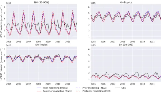
The mean time series of CH2O total columns for four latitu-dinal zones are shown in Fig. 6. XCH2O retrievals were not assimilated (contrary to the CH4and MCF surface measure-ments that affect the sources and sinks of CH2O in the in-version), and the inversion actually does not change XCH2O much. This suggests that the differences between simulated and satellite-retrieved XCH2Oare mainly caused by the prior NMVOC emissions used in the full chemistry run of LMDz-INCA. The latitudinal mean values of prior/posterior mod-elled XCH2Oagree fairly well with the OMI retrievals with-out any obvious bias, but the seasonal cycle is different, es-pecially in the northern mid–high latitudes both in phase and in amplitude (Fig. 6a). The OMI XCH2O retrievals, and the prior and the posterior simulations, all agree about the absence of a significant trend in the latitudinal average of XCH2O for the period from 2005 to 2011, which is consis-tent with the hypothesis that the equilibrium between the ox-idation of hydrocarbons into CH2O and the sink of CH2O into CO has not significantly changed, at least at continental scales. We note that the OMI XCH2Oretrievals describe some

trends at smaller scales, like positive trends of 3 ± 0.8 % yr−1 over East Asia (De Smedt et al., 2010) and negative trends of −1.9 ± 0.6 % yr−1over the Amazon, but they are not sig-nificant for the mean values of large latitudinal bands and are thus considered large enough to influence the global CO budget.

4.2 OH concentrations

Figure 7 shows the latitudinal average of the prior (blue) and posterior (red) OH concentrations for the six big regions over which OH is optimized (see Sect. 2.1). This figure reports the two inversions that use either TransCom-OH (solid lines) or INCA-OH (dashed lines; see Sect. 2.2.1). INCA has higher OH concentrations than TransCom in the NH, in particular during summer, but lower OH concentrations in the SH trop-ics all year long and slightly lower concentrations in the SH mid-high latitudes (south of 30◦S) during summer peaks.

In general, larger corrections are applied by the inversion to INCA-OH than to TransCom-OH. The inversion system adjusts the INCA-OH concentrations towards TransCom-OH by downscaling the OH concentrations in the NH during summers, especially over Asia, where INCA-OH is consider-ably higher than the TransCom-OH (Fig. 3). A small reduc-tion of the TransCom-OH concentrareduc-tions is also seen in the SH.

The two inversions do not produce significant trends in OH during the study period for most regions, except for a very small positive trend in the SH tropics (+0.2 % yr−1_with TransCom-OH and +0.7 % yr−1_{with INCA-OH) and a small} negative trend in the SH mid–high latitudes (−0.4 % yr−1in

TransCom-OH and −0.3 % yr−1 in INCA-OH). Such small

and insignificant trends are considered to be of minor impor-tance for the CO trends. The OH scaling is addressed in more detail in Sect. 5.1 when discussing CO sinks.

Figure 6. Time series of the CH2O total column averaged by latitudinal bands. The black lines indicate the CH2O total column from SAO OMI retrievals, green lines indicate prior simulations, and red lines indicate posterior simulations. Shading areas show the standard deviation within a latitudinal band. The forward and posterior simulations nearly overlay each other.

5 Optimized sources and sinks of CO

After having documented the prior and posterior misfits with MOPITTv6 and with cross-validation data for the latitudinal mean values and for the trends, which lends support to the consistency of the inversion results with these data streams, we now turn to the implications for CO sources and sinks.

5.1 Inverted CO budget

The global annual CO atmospheric burden, surface emis-sions, chemical production, and chemical loss of the prior and the posteriors with the two OH experiments from 2002 to 2011 are shown in Fig. 8. Averaging over the 10 years, a considerable increase in the mean CO atmospheric bur-den (+23 %, in dark green) is seen in the posterior compared to the prior simulation. Accordingly, increases in CO emis-sions (+50 %, in red) and chemical sinks with OH (+23 %, in purple) are produced in the posterior, whereas only a very small change is noticed for the CO chemical sources (+1 %, in blue). The magnitude of the increment in the global CO emissions is larger compared to previous studies that assim-ilate the 700 hPa retrieval levels of MOPITT using a similar inversion set-up (Fortems-Cheiney et al., 2011, 2012). The cross-evaluation against surface station measurements also shows a considerable positive bias in the posterior CO con-centration (Sect. 3.1), which implies a potential bias in the modelling of vertical CO profiles. Nevertheless, for our study here focusing on trends, such systematic model error does not seem to harm the robustness of the trends as shown in Sects. 3 and 4. The chemical sink of CO is a function of both CO and OH. Given the results for OH adjustments shown in

Sect. 4.2 (generally a small reduction from the prior OH), the increase in the CO sink in the posterior is thus mainly due to the increase in CO concentrations after assimilation.

The inversion produces a negative trend of around 10 % per decade in the global atmospheric burden

of CO (−5.1 ± 0.9 TgCO yr−1 with TransCom-OH and

−4.6 ± 0.8 TgCO yr−1with INCA-OH), which is twice the negative trend of the CO atmospheric burden produced by the prior emissions (−1.6 ± 0.6 TgCO yr−1, i.e. a decrease of 5 % per decade in the simulated CO burden).

For CO sources, the trend of prior CO emissions is of −11.1 ± 4.4 TgCO yr−1 (equivalent to a decrease of 10 % per decade). This is mostly contributed by the negative trend in biomass burning emissions in

GFEDv3.1 (−10.6 ± 3.7 TgCO yr−1) and by a very

small decrease in anthropogenic emissions in MACCity (−0.68 ± 0.4 TgCO yr−1)from 2002 to 2011. Compared to the prior emissions, a 2-fold steeper negative trend in terms of percentages is found in the posterior CO emissions, 24 % per decade with TransCom-OH (−40 ± 7.2 TgCO yr−1_{) and} 22 % per decade with INCA-OH (−37 ± 7.1 TgCO yr−1). A small positive trend (2.8 ± 7.1 TgCO yr−1, equivalent to an increase of 2 % per decade) is produced in the prior CO chemical production, mostly contributed by the increase in methane oxidation. The posterior CO chemical production shows a small negative trend. Yet, as CH2O concentrations are not constrained by observations, this small trend may result from the system’s inability to differentiate the two CO sources between surface emissions and chemical oxidations. For the CO sink, a larger trend in the posterior (−46.3 ± 8.3 TgCO yr−1, 16 % per decade) with

TransCom-Figure 7. Regional volume-weighted monthly mean OH concentrations in the prior and posterior. The results are shown for the six big

regions in which OH is optimized.

OH and −39.3 ± 8.0 TgCO yr−1, 13 % per decade with

INCA-OH is found, while there is no significant trend in the prior chemical sink. This negative trend in the posterior is mostly due to the decrease in CO concentrations in the atmo-sphere that change the amount of CO oxidized by OH, and only very small trends in the OH concentrations are found by the inversion. Such small trends are considered to have a very small effect on the CO trends. The OH concentrations are optimized for six big regions over the globe and the MCF concentrations are monitored at background sites only, which allows a coarse zonal estimate of OH but leaves spatially het-erogeneous land areas unconstrained, e.g. polluted areas near cities (Hofzumahaus et al., 2009), forests with high NMVOC emissions (Lelieveld et al., 2008) or biomass burning plumes (Folkins et al., 1997; Rohrer et al., 2014). Therefore, sub-regional trends in OH, if they exist, are not necessarily cap-tured in this study. In addition, with the exponential decrease of MCF concentrations in recent years (only a few parts per trillion, ppt, at the current level), the constraining strength of MCF on OH in the inversion system may not be even from 2002 to 2011, even though the same sites and a similar num-ber of observations were assimilated. Nevertheless, the zonal trend of OH should still be constrained throughout most of the period and previous studies suggest that the inter-annual change of global OH concentration is within 5 % (Montzka et al., 2011).

5.2 Regional distribution of trends in CO emissions

The distributions of trends in CO emissions after optimiza-tion are very consistent using either TransCom-OH or

INCA-OH (Fig. 9); therefore, only trends of TransCom-INCA-OH ex-periments are discussed here. The relative contribution of biomass burning to the total land surface emissions estimated in the prior emission is shown in Fig. 2b. The time series of the prior and the two posterior annual CO emissions us-ing two different OH fields are shown for each sub-region in Fig. 10. The division in sub-regions is illustrated in Fig. A1 in the Appendix. As shown in Fig. 10, the choice of prior OH concentrations could potentially have a large impact on the regional CO emission estimates; nevertheless, the inverted emission trends are quite robust and we do not discuss fur-ther in this paper the regional emission increments and the sensitivities of inverted fluxes to prior OH or chemical CO productions.

For the boreal regions where CO emissions are mainly due to biomass burning (boreal Asia – BOAS – and boreal North America – BONA), the same sign of the trends in CO emis-sions is mostly kept between the prior and the posterior, but the amplitudes of the trends are updated into larger values, as are the emission amounts. It should be noted that MOPITT CO retrievals over high latitudes beyond 65◦_{are not included}

in the assimilation.

For the NH mid-latitudes where CO emissions are mainly due to fossil fuel and biofuel burning emissions (USA; west-ern Europe – WSEU; eastwest-ern Europe – ESEU; Middle East – MIDE; South–Central Asia – SCAS; South-east Asia – SEAS), consistencies between the trends in the prior and posterior CO emissions are found in the developed countries (Fig. 9). For example, in the USA and WSEU regions, de-creasing trends produced by the emission inventories gen-erally agree with the atmospheric signals (Lamarque et al.,

Figure 8. Time series of global mean annual CO budget changes

from 2002 to 2011. Solid lines indicate the prior values (mean val-ues of the two OH fields are shown for the prior chemical CO pro-duction and sink). Dash-dot lines indicate posterior with TransCom OH and dotted lines represent posterior with INCA-OH. Beside each line, the linear slopes are denoted if the trend is statistically

significant,∗denotes the 95 % confidence level and∗∗denotes the

99 % confidence level.

2010). On the contrary, the inversion changes the sign of the CO trend over SEAS (including China) and SCAS (includ-ing India), where the prior emissions suggested a significant increase. Consistent with our posterior emissions, a grad-ual decrease in CO emissions in China after the year 2005 was actually deduced from CH4/CO2and CO / CO2 corre-lations observed off the coast of East Asia from 1999 to 2010 (Tohjima et al., 2014). A decrease in the emission factors of other co-emitted species of CO during fossil fuel or bio-fuel combustion has also been noted: for instance, a decrease in black carbon emission factors in China and India was re-ported by Wang et al. (2014), and a decrease in the relative ratio of NOxto CO2from 2003 to 2011 was observed from satellite retrievals over East Asia (Reuter et al., 2014). These studies and our results suggest that combustion technology improvements in East Asia resulted in emission factor reduc-tion to an extent that outweighs the impact of increasing fos-sil fuel burning. In this scenario, emission inventories would well report the latter but not the former, which is more dif-ficult to quantify. In addition, trends of fossil fuel emissions are updated (Lamarque et al., 2010), but not trends of bio-fuel burning, especially for traditional biobio-fuels (Yevich and Logan, 2003). A small difference in the trend of CO emis-sions in eastern Europe (ESEU) is also noticed (not

signifi-Figure 9. Trends distributions of CO surface emissions in the prior

and in the posterior from 2002 to 2011.

cant though); an emission peak in the year 2010 is inferred from the inversion.

For the tropical and sub-tropical regions, where CO emis-sions are mainly attributed to biomass burning, the inversion does not change the sign of trends over Indonesia (INDO). The positive trends of the prior emissions over the Indo-China Peninsula (2 % yr−1)are updated into negative ones (−5.6 % yr−1)by the inversion. Negative trends over Aus-tralia except for the central area (on average −5.3 % yr−1), and over SHSA (−3 % yr−1, but not significant for the re-gional mean) are largely enhanced compared to the prior trends (Fig. 9). The spatial distribution of this negative trend is consistent with the new version of GFEDv4 burned area (not used in this study) (Giglio et al., 2013), which accounts for small fires that were not explicitly included in GFEDv3.1 used here as the prior. In Australia, the decrease of CO emis-sions might be explained by decreased fire emisemis-sions (Poulter et al., 2014). The decrease in SHSA could be attributed to a decrease in deforestation fires in recent years, especially af-ter 2005 (Meyfroidt and Lambin, 2011), although there are

Figure 10. Annual prior (blue) and posterior (red) CO emissions in each sub-region from 2002 to 2011. The dash lines represent linear

regressions if the trend is statistically significant. The slopes are denoted beside the linear trends;∗and ∗∗represent significance at the

95 and 99 % confidence levels respectively. The notation for the sub-regions is listed as follows and the extent of each region is shown in Fig. A1. BOAS – boreal Asia; BONA – boreal North America; USA – USA; WSEU – western Europe; ESEU – eastern Europe; MIDE – Middle East; SCAS – South–Central Asia; SEAS – South-east Asia; INDO – Indonesia; AUST – Australia; NHSA – Northern Hemisphere South America; SHSA – Southern Hemisphere South America; NHAF – Northern Hemisphere Africa; SHAF – Southern Hemisphere Africa; OCEAN – all ocean emissions, both biogenic and anthropogenic emissions.

uncertainties in the overall deforestation rates (Kim et al., 2015).

The change in trends between the prior and posterior CO emissions is more heterogeneous over Africa (North-ern Hemisphere Africa – NHAF – and South(North-ern Hemisphere Africa – SHAF). Decreases in the burned area have been observed over the NHAF Sahel region, as are decreases in the prior CO emissions, which are explained by changes in both precipitation and the conversion of savannah into crop-land (Andela and van der Werf, 2014). But positive trends in CO emissions are inferred by the atmospheric inversion es-pecially since 2006, except for some small areas. The differ-ent signs of the trend in burned areas (or the prior CO emis-sions) and the posterior CO emissions may be explained by the change in CO emission factors that could vary a lot with the conversion of fire type from savannah fire to agricultural burning and also with precipitation change (van Leeuwen et al., 2013). In addition, increases in anthropogenic fossil fuel and biofuel emission in the NHAF region could also contribute to some of the differences (Al-mulali and Binti Che Sab, 2012). Differences between the prior and poste-rior CO emissions are also noticed for the central part of the SHAF. The increase in the GFED4 burned area is ex-plained by the increase in precipitation that allows more fuel accumulation, as driven by the El Niño–Southern Oscillation (ENSO) changes from El Niño to La Niña dominance over

the recent decade (Andela and van der Werf, 2014). The op-posite negative trend of CO emissions in the posterior could be explained by a decrease in CO emission factors when the fuel load and combustion completeness are high, so that less carbon is emitted in the form of CO, but the dynamics of emission factors are not modelled in the bottom-up estima-tion (van Leeuwen et al., 2013). In addiestima-tion, small fires that are not considered in our prior biomass emissions could also contribute to such differences (Randerson et al., 2012).

6 Conclusion

CO concentrations observed by both MOPITTv6 satellite XCO retrievals and surface in situ measurements show sig-nificant negative trends over most of the world from 2002 to 2011. The CO concentration trends in the forward CTM simulations prescribed with CO emission inventories show considerable inconsistency with the observed MOPITT XCO

from 2002 to 2011. By assimilating MOPITTv6 XCO and

surface measurements of CH4and MCF, the inversion sys-tem suggests that the decrease in the atmospheric CO con-centrations is mainly attributable to a decrease of 23 % in surface emissions during the study period at the global scale. The trends in the prior and posterior CO emissions agree well with each other over the USA and western Europe. The largest differences between the prior and the posterior CO

emission trends are noticed for South-east Asia, Australia and parts of South America and Africa. Decreases in CO emissions are found in central China, while the prior emis-sion inventories suggest increases. This emisemis-sion decrease is probably caused by a large decrease in emission factors due to technology improvements that outweigh the increase in emission activities. CO emissions from biomass burn-ing decreased considerably in Indonesia and Australia. For Africa, the contrasts of trends between the prior and the pos-terior likely reflect different trends between satellite-detected burned area and CO emissions due to changes in combustion completeness, CO emission factors, and the relative contri-bution of small fires. The amplitude of the trends also differs in many other regions, illustrating the original information brought by atmospheric inversions about CO emissions.

No significant trend is found in the latitudinal-mean OH

concentrations, and a sensitivity test made with two differ-ent OH fields suggests consistdiffer-ent results in the OH trend. It is however noted that we optimized OH over six big regions globally, and sub-regional trends in the OH concentrations, if they exist, are not accounted for in this study. We also ac-knowledge the limited information content of MCF to con-strain OH in recent years over the study period. For chemical

CH2O production from NMVOC oxidation, the system has

the potential to generate regional increments, but CH2O is not assimilated here due to limited temporal coverage of the OMI data from 2005 to 2011. Assimilating observations of CH2O and other chemically connected species could inform more about regional CO budgets, in particular the chemical sources and sinks, and therefore could further improve the top-down estimation of CO budgets for each region in future studies.

Appendix A

The Supplement related to this article is available online at doi:10.5194/acp-15-13433-2015-supplement.

Acknowledgements. The authors acknowledge the support of

the French Agence Nationale de la Recherche (ANR) under grant ANR-10-BLAN-0611 (project TropFire). F. Chevallier is funded by the European Commission under the EU H2020 Programme (grant agreement no. 630080, MACC III). The NCAR MOPITT and the SAO OMI retrievals are available from

https://www2.acd.ucar.edu/mopitt and http://disc.sci.gsfc.nasa.

gov/Aura/data-holdings/OMI/omhcho_v003.shtml, respectively.

We thank both institutes for having brought these data into open access and thank G. González Abad for helpful information about the OMI product. Similarly, we also acknowledge the WDCGG for providing the archives of surface station observations for

MCF, CH₄ and CO. We thank the following persons who have

participated in the surface in situ measurements through various networks: NOAA (E. Dlugokencky, G. S. Dutton, J. W. Elkins, S. A. Montzka, P. C. Novelli), CSIRO (P. B. Krummel, R. L. Lan-genfelds, L. P. Steele), EC (D. Worthy), Empa (B. Buchmann, M. Steinbacher, L. Emmenegger), JMA (Y. Fukuyama), LSCE (M. Ramonet), NIWA (G. Brailsford, S. Nichol, R. Spoor), UBA (K. Uhse), UNIURB (J. Arduini), and AGAGE (P. J. Fraser, C. M. Harth, P. B. Krummel, S. O’Doherty, R. Prinn, S. Reimann, L. P. Steele, M. Vollmer, R. Wang, R. Weiss, D. Young). Finally, we wish to thank F. Marabelle and his team for computer support at LSCE.

Edited by: A. Pozzer

References

Al-mulali, U. and Binti Che Sab, C. N.: The impact of energy

con-sumption and CO2emission on the economic growth and

finan-cial development in the Sub Saharan African countries, Energy, 39, 180–186, doi:10.1016/j.energy.2012.01.032, 2012.

Andela, N. and van der Werf, G. R.: Recent trends in African fires driven by cropland expansion and El Niño to La Niña transition, Nature Climate Change, 4, 791–795, doi:10.1038/nclimate2313, 2014.

Angelbratt, J., Mellqvist, J., Simpson, D., Jonson, J. E., Blumen-stock, T., Borsdorff, T., Duchatelet, P., Forster, F., Hase, F., Mahieu, E., De Mazière, M., Notholt, J., Petersen, A. K., Raffal-ski, U., Servais, C., Sussmann, R., Warneke, T., and Vigouroux,

C.: Carbon monoxide (CO) and ethane (C2H6) trends from

ground-based solar FTIR measurements at six European stations, comparison and sensitivity analysis with the EMEP model, At-mos. Chem. Phys., 11, 9253–9269, doi:10.5194/acp-11-9253-2011, 2011.

Arellano, A. F., Kasibhatla, P. S., Giglio, L., van der Werf, G. R., and Randerson, J. T.: Top-down estimates of global CO sources using MOPITT measurements, Geophys. Res. Lett., 31, L01104, doi:10.1029/2003GL018609, 2004.

Aumont, O. and Bopp, L.: Globalizing results from ocean in situ iron fertilization studies, Global Biogeochem. Cy., 20, GB2017, doi:10.1029/2005GB002591, 2006.

Bergamaschi, P., Hein, R., Heimann, M., and Crutzen, P. J.: Inverse modeling of the global CO cycle: 1. Inversion of CO mixing ra-tios, J. Geophys. Res., 105, 1909, doi:10.1029/1999JD900818, 2000.

Butler, T. M., Rayner, P. J., Simmonds, I., and Lawrence, M. G.: Simultaneous mass balance inverse modeling of methane and carbon monoxide, J. Geophys. Res., 110, D21310, doi:10.1029/2005JD006071, 2005.

Cammas, J.-P., Brioude, J., Chaboureau, J.-P., Duron, J., Mari, C., Mascart, P., Nédélec, P., Smit, H., Pätz, H.-W., Volz-Thomas, A., Stohl, A., and Fromm, M.: Injection in the lower strato-sphere of biomass fire emissions followed by long-range trans-port: a MOZAIC case study, Atmos. Chem. Phys., 9, 5829–5846, doi:10.5194/acp-9-5829-2009, 2009.

Chevallier, F., Fisher, M., Peylin, P., Serrar, S., Bousquet, P.,

Bréon, F. M., Chédin, A., and Ciais, P.: Inferring CO2

sources and sinks from satellite observations: Method and application to TOVS data, J. Geophys. Res., 110, D24309, doi:10.1029/2005JD006390, 2005.

Chevallier, F., Bréon, F.-M., and Rayner, P. J.: Contribution of the Orbiting Carbon Observatory to the estimation of

CO2 sources and sinks: Theoretical study in a variational

data assimilation framework, J. Geophys. Res., 112, D09307, doi:10.1029/2006JD007375, 2007.

Chevallier, F., Fortems, A., Bousquet, P., Pison, I., Szopa, S., De-vaux, M., and Hauglustaine, D. A.: African CO emissions be-tween years 2000 and 2006 as estimated from MOPITT observa-tions, Biogeosciences, 6, 103–111, doi:10.5194/bg-6-103-2009, 2009.

Cressot, C., Chevallier, F., Bousquet, P., Crevoisier, C., Dlugo-kencky, E. J., Fortems-Cheiney, A., Frankenberg, C., Parker, R., Pison, I., Scheepmaker, R. A., Montzka, S. A., Krummel, P. B., Steele, L. P., and Langenfelds, R. L.: On the consistency between global and regional methane emissions inferred from SCIA-MACHY, TANSO-FTS, IASI and surface measurements, Atmos. Chem. Phys., 14, 577–592, doi:10.5194/acp-14-577-2014, 2014. Deeter, M. N.: Operational carbon monoxide retrieval algorithm and selected results for the MOPITT instrument, J. Geophys. Res., 108, 4399, doi:10.1029/2002JD003186, 2003.

Deeter, M. N., Edwards, D. P., Gille, J. C., Emmons, L. K., Francis, G., Ho, S. P., Mao, D., Masters, D., Worden, H., Drummond, J. R., and Novelli, P. C.: The MOPITT version 4 CO product: Algorithm enhancements, validation, and long-term stability, J. Geophys. Res., 115, doi:10.1029/2009JD013005, 2010. Deeter, M. N., Martínez-Alonso, S., Edwards, D. P., Emmons, L.

K., Gille, J. C., Worden, H. M., Pittman, J. V., Daube, B. C., and Wofsy, S. C.: Validation of MOPITT Version 5 thermal-infrared, near-thermal-infrared, and multispectral carbon monoxide pro-file retrievals for 2000–2011, J. Geophys. Res.-Atmos., 118, 6710–6725, 2013.

Deeter, M. N., Martínez-Alonso, S., Edwards, D. P., Emmons, L. K., Gille, J. C., Worden, H. M., Sweeney, C., Pittman, J. V., Daube, B. C., and Wofsy, S. C.: The MOPITT Version 6 product: al-gorithm enhancements and validation, Atmos. Meas. Tech., 7, 3623–3632, doi:10.5194/amt-7-3623-2014, 2014.

De Smedt, I., Stavrakou, T., Müller, J.-F., van der A, R. J., and Van Roozendael, M.: Trend detection in satellite observations of formaldehyde tropospheric columns, Geophys. Res. Lett., 37, L18808, doi:10.1029/2010GL044245, 2010.

Duncan, B. N. and Logan, J. A.: Model analysis of the factors regulating the trends and variability of carbon monoxide be-tween 1988 and 1997, Atmos. Chem. Phys., 8, 7389–7403, doi:10.5194/acp-8-7389-2008, 2008.

Duncan, B. N., Logan, J. A., Bey, I., Megretskaia, I. A., Yan-tosca, R. M., Novelli, P. C., Jones, N. B., and Rinsland, C. P.: Global budget of CO, 1988–1997: Source estimates and val-idation with a global model, J. Geophys. Res., 112, D22301, doi:10.1029/2007JD008459, 2007.

EPA: National Trends in CO Levels, available at: http://www.epa. gov/airtrends/carbon.html, last access: 12 February 2015. Fisher, J. A., Wilson, S. R., Zeng, G., Williams, J. E., Emmons, L.

K., Langenfelds, R. L., Krummel, P. B., and Steele, L. P.: Sea-sonal changes in the tropospheric carbon monoxide profile over the remote Southern Hemisphere evaluated using multi-model simulations and aircraft observations, Atmos. Chem. Phys., 15, 3217–3239, doi:10.5194/acp-15-3217-2015, 2015.

Folberth, G. A., Hauglustaine, D. A., Lathière, J., and Brocheton, F.: Interactive chemistry in the Laboratoire de Météorologie Dy-namique general circulation model: model description and im-pact analysis of biogenic hydrocarbons on tropospheric chem-istry, Atmos. Chem. Phys., 6, 2273–2319, doi:10.5194/acp-6-2273-2006, 2006.

Folkins, I., Wennberg, P. O., Hanisco, T. F., Anderson, J. G., and

Salawitch, R. J.: OH, HO2, and NO in two biomass burning

plumes: Sources of HOxand implications for ozone production,

Geophys. Res. Lett., 24, 3185–3188, doi:10.1029/97GL03047, 1997.

Fortems-Cheiney, A., Chevallier, F., Pison, I., Bousquet, P., Carouge, C., Clerbaux, C., Coheur, P.-F., George, M., Hurtmans, D., and Szopa, S.: On the capability of IASI measurements to in-form about CO surface emissions, Atmos. Chem. Phys., 9, 8735– 8743, doi:10.5194/acp-9-8735-2009, 2009.

Fortems-Cheiney, A., Chevallier, F., Pison, I., Bousquet, P., Szopa, S., Deeter, M. N., and Clerbaux, C.: Ten years of CO emissions as seen from Measurements of Pollution in the Troposphere (MOPITT), J. Geophys. Res., 116, D05304, doi:10.1029/2010JD014416, 2011.

Fortems-Cheiney, A., Chevallier, F., Pison, I., Bousquet, P., Saunois, M., Szopa, S., Cressot, C., Kurosu, T. P., Chance, K., and Fried, A.: The formaldehyde budget as seen by a global-scale multi-constraint and multi-species inversion system, Atmos. Chem. Phys., 12, 6699–6721, doi:10.5194/acp-12-6699-2012, 2012. Giglio, L., Randerson, J. T., and van der Werf, G. R.:

Analy-sis of daily, monthly, and annual burned area using the fourth-generation global fire emissions database (GFED4), J. Geophys. Res.-Biogeo., 118, 317–328, doi:10.1002/jgrg.20042, 2013. González Abad, G., Liu, X., Chance, K., Wang, H., Kurosu, T. P.,

and Suleiman, R.: Updated Smithsonian Astrophysical Obser-vatory Ozone Monitoring Instrument (SAO OMI) formaldehyde retrieval, Atmos. Meas. Tech., 8, 19–32, doi:10.5194/amt-8-19-2015, 2015.

Granier, C., Bessagnet, B., Bond, T., D’Angiola, A., Denier van der Gon, H., Frost, G. J., Heil, A., Kaiser, J. W., Kinne, S., Klimont, Z., Kloster, S., Lamarque, J.-F., Liousse, C., Masui, T., Meleux, F., Mieville, A., Ohara, T., Raut, J.-C., Riahi, K., Schultz, M. G., Smith, S. J., Thompson, A., Aardenne, J., Werf, G. R., and Vuuren, D. P.: Evolution of anthropogenic and biomass burn-ing emissions of air pollutants at global and regional scales

during the 1980–2010 period, Climatic Change, 109, 163–190, doi:10.1007/s10584-011-0154-1, 2011.

Hauglustaine, D. A.: Interactive chemistry in the Laboratoire de Météorologie Dynamique general circulation model: Description and background tropospheric chemistry evaluation, J. Geophys. Res., 109, D04314, doi:10.1029/2003JD003957, 2004.

Hofzumahaus, A., Rohrer, F., Lu, K., Bohn, B., Brauers, T., Chang, C.-C., Fuchs, H., Holland, F., Kita, K., Kondo, Y., Li, X., Lou, S., Shao, M., Zeng, L., Wahner, A., and Zhang, Y.: Amplified trace gas removal in the troposphere, Science, 324, 1702–1704, doi:10.1126/science.1164566, 2009.

Holloway, T., Levy, H., and Kasibhatla, P.: Global distribu-tion of carbon monoxide, J. Geophys. Res., 105, 12123, doi:10.1029/1999JD901173, 2000.

Hooghiemstra, P. B., Krol, M. C., Bergamaschi, P., de Laat, A. T. J., Van der Werf, G. R., Novelli, P. C., Deeter, M. N., Aben, I., and Röckmann, T.: Comparing optimized CO emission estimates using MOPITT or NOAA surface network observations, J. Geo-phys. Res., 117, D06309, doi:10.1029/2011JD017043, 2012. Hourdin, F., Musat, I., Bony, S., Braconnot, P., Codron, F.,

Dufresne, J.-L., Fairhead, L., Filiberti, M.-A., Friedlingstein, P., Grandpeix, J.-Y., Krinner, G., LeVan, P., Li, Z.-X., and Lott, F.: The LMDZ4 general circulation model: climate performance and sensitivity to parametrized physics with emphasis on tropical convection, Clim. Dynam., 27, 787–813, doi:10.1007/s00382-006-0158-0, 2006.

IPCC: Abstract for decision-makers, in: Climate Change 2013: The Physical Science Basis. Contribution of Working Group I to the Fifth Assessment Report of the Intergovernmental Panel on Cli-mate Change, edited by: Stocker, T. F., Qin, D., Plattner, G.-K., Tignor, M., Allen, S. K., Boschung, J., Nauels, A., Xia, Y., Bex, V., and Midgley, P. M., Cambridge University Press, Cambridge, UK and New York, NY, USA, 2013.

Jiang, Z., Jones, D. B. A., Worden, H. M., Deeter, M. N., Henze, D. K., Worden, J., Bowman, K. W., Brenninkmeijer, C. A. M., and Schuck, T. J.: Impact of model errors in con-vective transport on CO source estimates inferred from MO-PITT CO retrievals, J. Geophys. Res.-Atmos., 118, 2073–2083, doi:10.1002/jgrd.50216, 2013.

Khalil, M. A. K. and Rasmussen, R. A.: Carbon monoxide in the Earth’s atmosphere: indications of a global increase, Nature, 332, 242–245, 1988.

Kim, D.-H., Sexton, J. O., and Townshend, J. R.: Accelerated De-forestation in the Humid Tropics from the 1990s to the 2000s, Geophys. Res. Lett., doi:10.1002/2014GL062777, 2015. Kopacz, M., Jacob, D. J., Fisher, J. A., Logan, J. A., Zhang, L.,

Megretskaia, I. A., Yantosca, R. M., Singh, K., Henze, D. K., Burrows, J. P., Buchwitz, M., Khlystova, I., McMillan, W. W., Gille, J. C., Edwards, D. P., Eldering, A., Thouret, V., and Nedelec, P.: Global estimates of CO sources with high resolu-tion by adjoint inversion of multiple satellite datasets (MOPITT, AIRS, SCIAMACHY, TES), Atmos. Chem. Phys., 10, 855–876, doi:10.5194/acp-10-855-2010, 2010.

Kurokawa, J., Ohara, T., Morikawa, T., Hanayama, S., Janssens-Maenhout, G., Fukui, T., Kawashima, K., and Akimoto, H.: Emissions of air pollutants and greenhouse gases over Asian re-gions during 2000–2008: Regional Emission inventory in ASia (REAS) version 2, Atmos. Chem. Phys., 13, 11019–11058, doi:10.5194/acp-13-11019-2013, 2013.