Defensive strategies in the quality ladders

HAL Id: halshs-00586709

https://halshs.archives-ouvertes.fr/halshs-00586709

Preprint submitted on 18 Apr 2011

HAL is a multi-disciplinary open access archive for the deposit and dissemination of sci-entific research documents, whether they are pub-lished or not. The documents may come from teaching and research institutions in France or abroad, or from public or private research centers.

L’archive ouverte pluridisciplinaire HAL, est destinée au dépôt et à la diffusion de documents scientifiques de niveau recherche, publiés ou non, émanant des établissements d’enseignement et de recherche français ou étrangers, des laboratoires publics ou privés.

Defensive strategies in the quality ladders

Ivan Ledezma

To cite this version:

WORKING PAPER N° 2008 - 29

Defensive strategies in the quality ladders

Ivan Ledezma

JEL Codes: L1, D2, O3

Keywords: innovative leaders, quality ladders, R&D,

regulation, industry-level data

P

-

S

E

L

’E

A

-

48,BD JOURDAN –E.N.S.–75014PARIS TÉL. :33(0)143136300 – FAX :33(0)143136310

Defensive Strategies in the Quality Ladders

Ivan Ledezmay

October, 2009

Abstract

This paper analyses the potentially defensive behaviour of patent race winners and its e¤ect on aggregate R&D e¤ort. It proposes a quality-ladders model that endogenously determines leader’s technology advantages and who innovates (the leader …rm or its competitors). Product market regulation can have either a positive or a negative e¤ect on R&D intensity. It can be negatively associated to aggregate innovative e¤ort in highly deregulated economies. In more regulated ones, where deterring strategies are constrained, it provides incentives to innovate. These predictions are consistent with data on manufacturing industries for 14 OECD countries during the period 1987-2003.

Keywords: industry-level data, innovative leaders, quality ladders, R&D, regulation. JEL Code: L1, D2, O3

I am grateful to Bruno Amable, Philippe Askenazy, José Miguel Benavente and Dominique Guellec for their helpful and detailed comments. I have also bene…ted from the reading and suggestions of Maria Bas and Elvire Guillaud. All remaining errors, of course, are my own.

y_{Centre d’Economie de la Sorbonne & Université Paris-Dauphine, LEDa-DIAL, 75775 Paris Cedex 16. Tel.}

1

Introduction

Several empircal studies based on R&D surveys show that …rms protect the value of their innovations using multiple strategies (Levin et al., 1987; Nelson and Walsh, 2000; Cohen et al., 2002). It is argued in this paper that this multiplicity is important to understand the e¤ect of competition on R&D incentives. If …rms have several alternatives to keep their pro…ts, potential competition may not necessarily act as a slack-reducing device. Rather than neutral innovative behaviour, the thread of competition can in practice trigger defensive reactions of incumbents. They can construct di¤erent types of strategic barriers aiming at protecting their business position from the risk of loosing future innovation contests.1 The aim of this paper is to analyse the impact of this defensive behaviour on aggregate R&D e¤ort and market structure. Particular attention is devoted to the way in which market regulation can in‡uence aggregate R&D e¤ort.

The paper …rst proposes a quality ladder model where R&D races are structured by strategic barriers, the cost of which is assumed to be positively correlated with regulation. Within a Stack-elberg game of the kind presented in Barro and Sala-i-Martin (2004), an important contribution of the model is that the new successful innovator strategically acquires R&D cost advantages vis-à-vis his competitors. These advantages allow him to further innovate. The main result is that regulation can have either a positive or a negative e¤ect on R&D intensity. It all depends on the pre-existing regulation level. In more liberal environments the equilibrium is charac-terised by a long-life innovative monopolist. Here an increase in regulation will be detrimental to innovation because it distorts the innovative activity of the leader. However, after attaining a certain threshold of regulation, the economy experiments Schumpeterian replacement. In this case, regulatory provisions can positively in‡uence aggregate R&D e¤ort since they reduce the deterring e¤ect on outsiders. Because of Schumpeterian incentives stemming from the technol-ogy gap between leaders and followers, this positive impact is all the more important that the size of innovation is bigger.

The starting point to understand these results is to conceive regulation as a device con-straining the set of available strategies, namely those leading to entry deterrence in R&D. In the model this kind of strategies are illustrated by the choice made by the leading …rm regarding the direction of the innovative path. The idea is that innovation is not only a purely product/process

1

Consistent with R&D surveys …ndings, Crépon and Duguet (1997) show evidence of negative R&D external-ities among French manufacturing …rms in narrowly de…ned industries, a result interpreted by the authors as the outcome of competitors’rivalry.

improvement but a strategically “biased”one. Regulation can (de facto) limit the possibilities of technological manipulation (think in certi…cations, anti-bundling, quality controls, certi…cations, licensing, etc). An important point is that even some usually-called market barriers can …t this de…nition. Theoretically speaking, all that is needed is a rule that directly or inderectly sets the boundaries of the business process and product containing the state-of-the-art knowledge. This is why the empirical excercise deliberatly uses indicators constructed to measure market barriers.2

Model’s predictions are tested using industry-level data of OECD countries for the period 1987-2003. Several indicators of regulation provided by the OECD appear positively correlated with R&D intensity in high-tech industries, precisely those industries where the size of innovation usually yields big innovative jumps. Consistent with the model, once the sample is split to investigate a di¤erentiated e¤ect of regulation on R&D intensity, a negative correlation shows-up in highly deregulated environments. The opposite is observed in more coordinated ones.

These empirical results are themselves new interesting evidence that the paper helps to ex-plain. As surprising as it may be, they are broadly consistent with previous studies at the industry level. Most of them, explore the link between regulation and economic performance by relying on OECD regulation indicators (as in this work). Nicoletti and Scarpetta (2003) report a positive interaction between product market regulation and the proximity to the technology frontier in a model explaining multifactor productivity growth. While the authors interpret their …nding as a negative e¤ect of regulation on the catching-up process, it also implies that the impact of regulation on productivity growth positively increases with the proximity to the frontier. Similarly, Amable et al. (2009) …nd no evidence of a negative e¤ect of regulation on innovative performance close to the technology frontier. After several robustness checks, what remains is that the marginal e¤ect of regulation on innovation tends to be positive at the lead-ing edge.3 Inklaar et al. (2007) analyse several sources of multifactor productivity growth in service sectors. Excepting telecommunications, their results fail to show a robust negative e¤ect of market barriers indicators on productivity growth. On the other hand, Arnold et al. (2008)

2

The Economist in the title of the printed article of May 1st 2008 re‡ects the non-trivial link between regulation and competition: "Oceans Apart: Europe still seems to have less faith than America in the ability of the free market to tame monopolies".

3

These industry-level works contradict micro-level results found by Aghion et al. (2005) for a panel of UK …rms using pro…tability-based measures of competition. The inverted-U shape pattern between competition and innovation, that underlies Aghion et al.’s (2005) claim, has also been empirically relativised at the micro-level by Tingvall and Poldahl (2006). A number of theoretical arguments, dealing with strategic behaviour, can be mentioned to explain the lack of clear-cut results on this matter (see for instance Etro 2007, Chapter 4; Tishler and Milstrein, 2009; Amable et al. 2009;)

do report that regulation induce a negative e¤ect on …rm productivity, but only in ICT-using industries. Among them, their sample considers several service sectors which are not present in the manufacturing sample used in this paper. Gri¢ th et al. (2006) investigate the e¤ect of the Single Market Programme (SMP) on R&D expenditure. Di¤erently from the previously men-tioned empirical works, the authors construct indirect indicators of market regulation through a step function that, basically speaking, seeks to measure the expected exposition to the SMP. Pro…tability e¤ects of regulation are isolated following a two-step methodology. Results are that the liberalisation trend induced by the SMP is positively correlated with R&D investment. However, in line with the results presented in the present work, in several of R&D reduced-form regressions (i.e. including other chanels than pro…tability) and also in some of the robustness check TFP regression, the group of industries related to the catgeory of "high-tech public pro-curement" (including telecommunications equipment, o¢ ce machinery and medical and surgical equipment) presents a signi…cantly negative correlation, that is to say, a negative impact of deregulation on R&D and productivity.4

The theoretical explanation proposed by the paper brings some standard developments of industrial organisation (IO) into a quality-ladders growth setting. Whilst strategic entry deter-rence and preemption in R&D races have been deeply analysed in IO works they have received much less attention in Schumpeterian growth models until recently.5 _{Some exemples include}

ex-plicitly defensive behaviour of incumbents such as the introduction of tacitness in the knowledge embodied in production techniques in order to prevent leapfrogging (Thoenig and Verdier, 2003) or the engagement in patent blocking, intelectual property disputes and the like to delay their replacement (Dinopoulos and Syropoulos, 2007). In such papers …rms play simultaneously in a Nash-Cournot equilibrium and have symmetric technologies in R&D. These assumptions imply that Arrow replacement e¤ect holds and leaders do not continue to innovate. There is however, convincing evidence about the active rôle of leaders in R&D (see for instance Chandler, 1990; Malerba et al., 1997). In the proposed model, the participation of the leader in R&D contests arises endogenously.

The circumstances under which the Arrow e¤ect vanishes has also been addressed in early

in-4

Other related evidence is that provided by macro-institutional literature emphasising the diversity of capi-talism (Albert, 1991, Hall and Soskice, 2001; Amable, 2003). Di¤erent institutionals con…gurations are able to deliver economic performance. In some of them, market-based forces ensured by a deregulated environment are the key dynamic engine, in other it is rather institutional coordination and welfare state that are associated to economic performance. The evidence provided later is broadly compatible with this line of research.

5_{Bain (1949), Williamson, (1963), Salop (1977), Dasgupta et al. (1982), Gilbert and Newberry (1982) and}

‡uent models of patent races but only recently spanned into quality-ladders literature.6 _This

de-…ne a special class of models able to reproduce innovative leaders. This can be done, for instance, thanks to the assumption of exogenous R&D advantages either within Nash-Cournot equilibri-ums and decreasing returns in R&D technology (Segerstrom and Zolnierek, 1999; Segerstrom, 2007) or within a Stackelberg type game (Etro, 2007 & 2008) that can be represented in a simple version with constant returns in R&D (Barro and Sala-i-Martin, 2004-Chapter 7). These works, however, consider innovation contests where the asymmetry betwen the R&D technology of the leader and that of the follower is exogenous. The explanation proposed here links these models with the above mentioned category by reproducing endogenous relative R&D advantages of leaders through defensive strategies. Introducing a stage in which R&D asymmetries can be acquired renders more sounding the …rst move advantage game.7

Similar strategic issues has been recently analysed by Grossman and Steger (2008). They show, that from the leader’s point of view, the erection of entry barriers and R&D are comple-mentary activities. Despite entry blocking, this behaviour can be conductive to positive growth e¤ects when outsiders’R&D do not generate knowledge spillovers. Important di¤erences exist between their model and the one presented in this paper: Cournot versus Bertrand competition here, deterministic innovation versus risky R&D investment here, a rather static entry bar-rier construction versus path dependency here (among others). This makes comparisons hard. Their results are, however, compatible with the equilibrium with permantent monopolist. Over-all, what should be kept in mind is that, rather than render the analysis ambiguous, the richness of IO tools provides a highly selective level of robustness scrutiny. It is then not surprising to conclude that the relationship between competition and innovation remains an open question.

The rest of the paper is organised as follows. Section 2 presents the model and Section 3 the empirical …ndings. Finally, concluding remarks are presented in Section 4. In order to keep the exposition simple, most of technical developments is presented in appendix.

6_{For patent races works, see for instance the interesting discrepancies between Gilbert and Newberry (1982)}

and Reinganum (1983).

7_{An alternative line of argument is that of Denicolò (2001). If innovation is non-radical, the gap in the industry}

can be such that the leader may practice a monopolist price while the next competitive outsider engage in Bertrand competition with consequently lower incitations. As knowledge spillovers, specially in high-technology industries, may constrain the sustainable technology gap between …rms, the explanation of R&D advantages is put forward in the present work. Even if small, these R&D cost advantages justify that the leader continuously invests in R&D (Klette and Griliches, 2000).

2

The model

For the sake of simplicity, the formal setting is based on a semi-endogenous quality-ladders model without scale e¤ects. The basic setup is based on Li (2003) which generalises Segerstrom’s (1998) framework. It considers imperfect inter-industry substitutability and remove steady state scale e¤ects by assuming that, as quality improves, new discoveries need more R&D e¤ort. At equilibrium the innovation rate will not depend on the size of labour allocated to R&D but on the rate of population growth.8

Section 2.1 begins presenting the rationale of the model, 2.2 follows with the basic setup of consumption and production. The core of the setting is then presented: the strategic use of private knowledge and capabilities (Sections 2.3 and 2.4) and the e¤ects on aggregate R&D e¤ort at equilibrium (Section 2.5).

2.1 The model in words

The model consists of two main ingredients: (i) an endogenous choice of technological bias and (ii) a Stackelberg type game in which the leader has the …rst mover advantage. Through a vectorial representation, the leader (i.e. the new succesful innovator) is assumed to chose its level of R&D investment but also the speci…c quality mix to be introduced into the market. By changing the latter, the new incumbent introduces a "technological bias" in the direction of the innovation path and obtains R&D cost advantages that are crucial in the Stackelberg game. Challengers are compelled to provide a new business solution in the context of several disadvantages concerning learning, experience, lead time developing, lack of codi…cation, etc. (for short knowledge ) as well as unfavourable conditions related to the need of new manufac-turing complementarities, patents and licenses, agency and organisational issues, market access, etc.(for short capabilities).9 _{The leader, by carefully choosing the speci…c charcateristic of the}

good, exploits these assymetries in knowledge and capababilities.10

8

This feature characterises a second wave of quality-ladders models that solve problems of scale e¤ects in the steady state growth (Segerstrom, 1998; Young, 1998), a property strongly contradicting empirical evidence found by Jones (1995): while resources allocated to R&D increase exponentially in the long-run data, productivity growth remains almost constant. For a survey on the evolution of this type of schumpeterian models see Dinopoulos and Sener (2007).

9_{For instance, Intel Inside has recently incorporated the hafnium, a new material allowing to concentrate more}

transistors into their microchips (45 nm processors) . This requires investments in manufacturing adaptations that give the upper-hand of Intel over its rivals.

1 0

Simulating a model of management search, Rivking (2001) shows that complexity can account for the di¤erence between replication and imitation. At certain level of complexity, neither low nor high, the incumbent is able to replicate a succesfull strategy within the boundaries of the …rm with much less di¢ culties than its competitors can imitate it.

Regulation is usually modeled as a …xed entry cost without other consequence than the misallocation of ressources. Here, product market regulation increases the cost of technological bias. This cost of course negatively in‡uences the leader …rm value at the entry. However, it has consequences on the properties of the new good and as such, it indirectly acts as a knowledge codi…cation device. Not only antidumping measures might do this job, but also other regulatory provision that might look like product market barriers (certi…cations, licences, product limitations, quality controls and the like).

The Stackelberg building block closely follows Barro and Sala-i-Martin (2004). Outsiders can be driven away from R&D races if the leader makes a commitment of high R&D investment. The credibility of this commitment relies on the (acquired) leader’s technological advantages, constrained in…ne by regulation. Thus, the model yields a threshold that de…nes who innovates. If the leader …rm is not credible, the Arrow replacement e¤ect holds in the usual way: outsiders have more R&D incentives than incumbents, because the latter must replace themselves. As a consequence, potential entrants carry out all R&D e¤ort and an steady state equilibrium with continuous Schumpeterian replacement (SR) takes place. In such equilibrium, the technological bias helps the incumbent to delay its ending date. On the contrary, if the leader …rm can make a credible commitment, it will do all R&D and will remain in the market inde…nitely in the context of a permanent monopolist (P M ) equilibrium.

Each equilibrium accounts for a di¤erent e¤ect of regulation. In the SR equilibrium, regula-tion increases the share of labour allocated to R&D because it limits entry deterrence. Its e¤ect, however, depends positively on the size of the innovative steps as it represents a monopolistic premium modulating R&D incentives. On the contrary, in the P M equilibrium if regulation increases it reduces R&D intensity. The reason is that, within this equilibrium regulation con-sumes more labour for defensive purposes without creating enough incentives for outsiders’R&D investment.

2.2 Consumption and production

2.2.1 Consumption: instantaneous decisions

Per capita utility at each time t is given by the CES formulation:

u (t) = 2 4 1 Z 0 z (t; !) 1 d! 3 5 1 (1)

z (t; !) P_j j_{d (j; t; !) is the sub-utility function associated to each industry !. The}

demand for the good of quality j at time t in industry ! is denoted by d (j; t; !). The term j captures the quality level j of a given good, where > 1 is a parameter representing the size of quality upgrade. Thus, within a given industry consumers preferences are ordered by the quality of the available varieties. To avoid confusions in notation, all round brackets, () ; are reserved to the arguments of the functions of the model.

At any time, households allocate their consumption expenditure E (t) seeking to maximise u (t). This static problem can be separated in two components: a within-industry consumption decision and a between-industry one. Giving the utility function z (t; !) for the quality varieties in each industry !, all intra-industry expenditure will focus on the good j having the lowest quality-adjusted price: j = arg min

(j)

p( j_;t;!)

j :

The between-industry problem concerns the allocation of total expenditure E (t) among all ! 2 [0; 1]. This consists of applying the optimal intra-industry demand z (t; !) = d (j ; t; !) to (1) and maximising u (t) subject to

1

Z

0

p (j ; t; !) d (j ; t; !) d! = E(t), which leads to the well-known CES demands:

d (j ; t; !) = (j ; t; !) p (j ; t; !) 1 R 0 (j ;t;!0) p(j ;t;!0)1 d!0 E(t) (2)

Where (j ; t; !) j [ 1] _{is a quality level index.}

2.2.2 Consumption: intertemporal decisions

Households are identical dynastic families whose number of members grows at the exogenous rate n > 0. Each member of a household supplies inelastically one unit of labour. Without loss of generality, initial population is set to 1, so that the population at time t is L(t) = ent_{. Using}

a subjective discount rate > n; each dynastic family maximises its intertemporal utility

U = 1 Z 0 e [ n]tlog u (t) dt (3) subject to a (t) = w (t) + r (t) a (t) E (t) na (t)

Where the intertemporal budget constraint links stock market gains, revenue and expendi-ture. a (t) is the endowment of per capita assets. Its variation a (t) is decomposed into current

wage income of the representative household member w (t) plus stock market gains r (t) a (t) minus expenditure E (t). Between t and dt, the growth of per capita assets needs to be adjusted by population growth n. Observe that u (t) = E(t)_P ; where P =

1 R 0 h p(j ;t;!0₎ j i1 d!0 1 1 is the utility-based price index. Since P is taking as given, the problem is equivalent to maximise U =

1

Z

0

e ( n)t_{log E (t) dt subject to the intertemporal budget constraint. Solving this program}

leads to the well-known intertemporal optimal rule:

E (t)

E (t) = r (t) (4)

2.2.3 Producers and price setting

Labour is the only factor in production and is used in a technology with constant returns to scale. Each …rm producing the variety ! sells its output to all members of the representative household. Thus, the …rm produces a quantity of d (j ; t; !) L (t) ; sells at price p (j ; t; !) and incurs a production cost w (t) d (j ; t; !) L (t). After wage normalisation, w (t) = 1; the pro…t of each producer is given by:

(j ; t; !) = [p (j ; t; !) 1] d (j ; t; !) L (t) (5)

Standard monopolist pro…t maximisation would lead to a markup over marginal costs: p (j ; t; !) = ₁. However, the monopolist is also in competition with …rms o¤ering lower quality goods. Bertrand competition yields to a limit pricing behaviour. Consider, namely, a …rm laying one step behind the leader in the quality-ladder and whose best quality-adjusted price is p(j j 1;!;t)1 =

1

j 1 (i.e. its price equals its marginal cost). The leader …rm will then

charge p (j ; !; t) = and get all demands.11

The application of this intra-industry price setting will depend on the size of innovation and the monopolist power ₁. If ₁ > …rms will charge p (j ; !; t) = . On the contrary, if

1 the leader is unconstrained to charge its optimal monopolistic price rule p (j ; t; !) = 1. This introduces the following assumptions:

Assumption 1 Price setting is constrained by potential entry ₁ > , so that p (j ; !; t) = p = :

1 1

A tie-break rule assumption, stating that a consumer facing similar quality-adjusted prices prefers the good with the highest quality, allows to avoid the use of a quality-adjusted price in…nitesimally lower.

Assumption 2 Knowledge spillovers are such that any time an innovative …rm succeeds, the previous version of the good is available for the rest of …rms.

The model works with further quality upgrades of the same good. In this sense, it is more plausible to suppose, as in Assumption 1, that the size of each upgrade is not big enough to induce the innovator to adopt the same price behaviour than a monopolist having no outside competition. Assumption 2 implies that there always be a …rm one step down so that the only possible price setting is this bounded limit price.12

Putting demands (2) into leader pro…ts (5) and using the fact that p neither depends on j nor on ! yields: (j ; !; t) = [p 1] p (j ; !; t) Q (t) E (t) L (t) (6) Where Q (t) 1 R 0 (j ; !; t) d! = 1 R 0

j [ 1]_{d! is the average quality index. Thus, the}

monop-olistic competition framework implies that …rms compete in quality with the whole economy.

2.3 R&D technologies and quality improvements

At each state-of-the-art quality level j; the successful innovator of the current R&D race improves quality to the level j + 1 and climbs the quality-ladder one step up.13 _{The above-exposed price}

setting implies that the successful innovator becomes the sole producer in the industry. Thus, each incumbent is also the monopolist and the leader of the industry. Di¤erently from the standard setup, in this model the incumbent does not wait until the next innovator "steals" its rents, but seeks to deter its potential rivals and to remain in the market. This section is devoted to set the underlying R&D framework allowing for these mechanisms. Before starting a subscript simpli…cation can be made.

Subscript simpli…cation Observe that: (i) there is only one …rm producing a positive quantity in an industry; (ii) the only di¤erence among industries concerning state variables is the current state-of-the-art quality level j; and (iii) all endogenous variables depend on t (except prices). Based on (i) and (ii), j! will now summarise the couple (j ; !) ; which indicates the

1 2

Further consequences of this assumption are discussed in section 2.4.1.

1 3_{Within a symmetric equilibrium, it is usually supposed that, at t = 0, the state-of-the-art quality in each}

industry is j = 0 and that some producer has the knowledge to fabricate a good of quality j = 0: Firms then engage in R&D races to discover a new version of the good.

current state-of-the-art good produced by the leader of industry !. Thanks to (iii) the time index can be dropped, keeping in mind the time dependency of the model.

2.3.1 Quality dimensions

The quality provided by a …rm producing in industry ! is given by the quality vector !q (j!) =

fq1(j!) ; q2(j!) :::; qm(j!)g . These m dimensions concern not only the fabricated good but also

the whole business process involved in the provision of the good to the customer and related services (i.e. the integrated supply chain). The magnitude (level) of quality is summarised by the euclidean norm of the vector k!q (j!)k =

s

m

P

k=1

q_k2(j!) and the quality mix by its direction

(the angle of the vector), which re‡ect the composition of the o¤ered good. In line with the intra-industry sub-utility function, di¤erent mix concerning the same industry and quality level are also perfect substitutable versions of the same product. In each industry, two di¤erent quality mix provide the same utility if their magnitude is equal. Direction only matters in the research sector.

The quality state j!is the outcome of step-by-step innovations. The magnitude of the quality

vector is upgraded at each step by a factor of ; the size of innovations. The quality provided by the state-of-the-art j! is thus de…ned as k!q (j!)k = j!:

2.3.2 R&D technologies

The de…nition of R&D technologies is based on two assumptions:

Assumption 3. While outsiders competing in a R&D race take the current quality mix as given, the current successful innovator can change it.

Assumption 4. Outsiders take a time to acquire the knowledge and capabilities to introduce a new dimension of quality into the new state-of-the-art product.

Assumption 3 re‡ects the innovator’s advantages arising from its private knowledge about the new product. Once the new discovery come o¤, the new blueprint is certainly known by the innovator. The leader …rm now has the choice about what visible properties its product and related services will have in the market. Assumption 4, implies that outsiders need to develop additional knowledge and capabilities to be able to replicate and improve the current state-of-art knowledge.14

1 4

Outsiders’R&D technology Outsiders carry out R&D activities by using labour as input. R&D is governed by a Poisson stochastic process: `i units of labour allocated to research during

an interval of time dt imply a probability of success 0(j!+ 1) `idt of a new upgrade. The R&D

productivity is the augmenting factor of the probability of innovative success implied by one unit of labour in the R&D process. For the outsider, the R&D productivity is de…ned as

0(j!+ 1)

h cos j!

(j!+ 1)

Following Li (2003), this R&D productivity is a function of the upgrade endeavoured (j!+ 1).

The presence of the quality index (j!+ 1) = [j!+1][ 1] represents the idea that, as the level

of quality increases, the next improvement becomes harder and R&D more costly. h is an exogenous technological parameter of R&D e¢ ciency.

The incidence of the quality mix on R&D is captured by the normalised scalar product between the current and the previous quality vector (i.e. between !q (j!) and !q (j! 1)),

which is completely de…ned by the angle j! between both vectors. That is to say:

!_{q (j!)} !_{q (j! 1)} k!q (j!)k k!q (j! 1)k

= cos j!

Recall that the cos ( ) function is symmetric and monotonically decreases from 1 to 0 along with j j!j 2 [0; =2[ (in radians). Hence, a change in the quality mix at quality state j! (i.e.

j!) increases the R&D di¢ culty faced by outsiders by a factor cos j!, where > 0 captures

the impact of the thecnological bias. The instantaneous probability of innovation Ii implied by

the R&D e¤ort of outsider i is then:

Ii= `i

h cos j!

(j!+ 1)

(7)

The advantage of using a vectorial representation of quality is that, between two wave of innovations, quality dimensions need not be speci…ed. Between the previous and the current version of the product, represented by two vectors of Rn; all the information needed is the angle between them. The e¤ect of technological bias collapses to the scalar product among both vectors.

state of knowledge to mount their own research e¤ orts, even if the patent laws (or the lack of complete knowledge about best production methods) prevent them from manufacturing the current generation products" (Grossman and Helpman, 1991 p. 47). The "lack of complete knowledge" can be related to the way in which a new mix of quality must be incorporated into the new good, as well as the need of solutions to overcome the barrier constructed by the incumbent.

Leader’s R&D technology The leader …rm does not face the di¢ culty coming from bias. It has discovered the current state-of-the-art product and it is the sole producer that knows how to incorporate the new dimension in the manufacturing of the good. Hence, the leader’s R&D productivity is:

L(j!+ 1) =

h (j!+ 1)

2.3.3 The path of innovation and regulation

As a way to protect their position, the innovator can add a new quality dimension to the cur-rent mix in order to introduce a bias in the path of innovation. The model assumes that the discovery enables the innovator to incorporate some new component or process that exploit its asymmetries in knowledge and capabilities. This new dimension can include, for instance, new services, bundling, speci…c intermediate inputs, manufacturing installations, property rights, market access, vertical integrations, etc. introduced with the aim to take advantage from their complementary assets, know-how and technology. It can also be the "re-discovery" of a tradi-tional dimension that have been dropped in the previous version of the good and for which the way to be included in the new version is by no means widely feasible because of compatibility issues or/and licensing contracting.15

Figure 1 illustrates the path of innovation. Let us start from the quality level j in a given industry. At this stage thee good is totally based on dimension q1(implying a horizontal vector).

Once the next innovative …rm has succeeded in upgrading the quality level to j + 1; it introduces a bias by including dimension q2: The …rm then produces the new version of the product with a

quality vector having a direction j+1 far away from the previous one. By doing so, it increases

the di¢ culty of the next R&D race (the one leading to the j + 2 level) by a factor of cos j+1:

Then, the next innovation occurs and improves the quality level to j + 2 and do the same: Since at each discovery new dimensions are available, this process may last inde…nitely. The …gure suggests a case for "re-discovery" of quality dimensions. The new mix at stage j + 2 lies completely on the plan q2 and q3: Dimension q1 has been dropped (q1(j + 2) = 0). If some

com-patibility concern arises after one step, the next incumbent ( the winner of the j + 3th contest) can use again the quality dimension q1 as a source of bias.

1 5_{Think for instance in Dolby audio technology compatible with i-Pods or, even, in the o¤er of organic ice}

Figure 1. Innovation Path

Any leader that changes the mix incurs a variable cost (in units of labour) of adapting the new version. This cost is de…ned through the following functional form :

c ( j!; )

f

cos j! L(j!)

(8) where > summarises the extent to which product market regulation limits the new version of the product. Regulation implies a cost of technological bias that increases with the change of the direction of the quality vector. Thus, in this illustration regulatory provisions are modeled as limiting complexity in the manufactured version of the improved product. The assumption > means that regulation is supposed to be e¤ective in limiting the new incumbent.

The cost of introducing a technological bias in the new product diminishes with the R&D productivity involved in its discovery. This captured by the term L(j!) : the R&D productivity

of the leader …rm in the former R&D race j! (the one that it has won). The presence of

L(j!) also implies that higher quality goods are more di¢ cult "to bias" since R&D productivity

decreases with the quality level of the industry. This rather realistic assumption helps to simplify the dynamics of j!. Finally, a cost parameter f is included to take into account the measure

2.4 Strategic behaviour

2.4.1 Stochastic jumps and timing

If researchers of an outsider …rm i succeed, the …rm get a value denoted by vL(j!+ 1) : Free entry

in the research sector implies that …rms enter up to the point where the expected value of inno-vation, vL(j!+ 1) o(j!+ 1) `iodt; equates the R&D e¤ort `io invested during the in…nitesimal

interval of time dt. That is to say :

vL(j!+ 1) =

1

o(j!+ 1)

(9)

Given the CRS in R&D technology, the R&D e¤ort of the outsider for a given value of a successful innovation vL(j!+ 1) is then:

`io = 8 > > > > < > > > > : 0 if vL(j!+ 1) < <sub>o(j</sub>1<sub>!+1)</sub> 1 if vL(j!+ 1) > <sub>o(j</sub>1<sub>!+1)</sub> `io2 R+ if vL(j!+ 1) = _o(j1_!+1) (10)

Let `0 =P<sub>i</sub>`i0be the total amount of R&D carried out by outsiders. The Bellman equation

of a (potential) innovative leader can be written as

rvL(j!) = L `L+ `L L(j!+ 1) [vL(j!+ 1) vL(j!)] (11)

`o o(j!+ 1) vL(j!) c ( j!; )

If the leader invests `L in R&D, with instantaneous probability `L L(j!+ 1) its optimal

value vL(j!) can jump to vL(j!+ 1) thanks to the new discovery. With instantaneous

proba-bility `o o(j!+ 1) the leader may be replaced by a successful outsider. In the meantime, the

leader …rm enjoys its monopolist pro…ts L and pays `L unit of labour for new discoveries as

well as c ( j!; ) units of labour for defensive strategies.

16

Assumption 2 implies that the maximum gap attained is one step. Therefore, an asymmetry in price setting incitations will not arise here. Even if the leader innovates it will not get enough technological distance to practice a monopolistic price that would give him more incentives to innovate compared to an outsider that must charge a Bertrand price when innovations are

non-1 6

Equation (11) implicitly says that the current value of a follower is zero. This is the result of Bertrand competition, the free entry condition with CRS and zero R&D sunk cost to be payed before playing.

radical (see Denicolò, 2001). This assumption allows to focus, by construction, on incitations stemming from R&D advantages.

Built on this setting, the timing of the model is as follows:

1. Nature : At the very beginning of the technological state j!, the nature provides the leader

(the current successful innovator), symmetric R&D technologies and the parameters of the model, namely the level of regulation. Free entry in the research sector applies.

2. Entry into the product market : the leader chooses the level of bias j! in order to maximise

its value. It takes the parameters of the model as given, namely the level of product market regulation. Production starts.

3. R&D race :

(a) The leader decides its optimal level of R&D e¤ort `Ltaking j! as …xed and knowing

outsiders reaction (10)

(b) Having observed the leader’s commitment `L, outsiders set their optimal R&D e¤ort

`o

Once investments are engaged, they remain …xed during the contest. Namely, the leader cannot change its choice of j!. The ‡ow cost c ( j!; ) can then be seen as the amortised

defensive investment per-time interval dt. Stage 3 is the core of the Stackelberg game based on Barro and Sala-i-Martin (2004) model. A key di¤erence is that the relative cost advantages are endogenous thanks to stage 2.

2.4.2 The Stackelberg game

The following proposition establishes the conditions under which outsiders are deterred. The presentation focuses on the case where j! = is constant. In section 2.3.3, this will prove to be

true for a constant outsider menace, which is the standard steady state condition of this kind of model.

Proposition 1 For a constant value of j! = ; a su¢ cient condition to ensure a non pro…table

R&D e¤ ort for outsiders is

cos h

1 [ 1]

i

Under this condition, the leader’s R&D e¤ ort can be positive and irrespective of outsider actions. In this equilibrium the leader value and the interest rate verify, respectively

vL(j!) = L c ( ; ) r (13) r = p 1 p E L 1 [ 1] h Q (14)

Proof. See Appendix A.1.1.

The inequality stated in (12) will be referred to as the credibility condition. Intuitively, it de…nes a threshold for the R&D productivity advantage of the leader L(j!+1)

o(j!+1) =

1 cos ;

which is increasing in (i.e. decreasing in cos ). This threshold determines whether the R&D investment is pro…table for the leader …rm (i.e. whether it is credible). If this is the case, constant returns of R&D investment imply that the leader can potentially perform enough R&D e¤ort to put outsiders out of competition. Thus, when the bias is strong enough, the leader does carries out research e¤ort and the outcome is that the value of the next quality improvement is lower than the R&D cost incurred by outsiders vL(j!+ 1) < _o(j1_!+1) (see the

proof of Proposition 1 for details). As a consequence, outsiders react by setting zero R&D e¤ort, meaning no replacement menace: Io =PiIio = 0. In this case the leader value is given by (13).

In contrast, if the credibility condition does not hold, the leader will be replaced and all R&D will be done by outsiders. Its value in such a situation is that implied by (11) for `L= 0: The

ex ante value of the incumbent can be summed up as:

vL(j!) = 8 > < > : L c( ; ) r+`o o(j!+1) if cos > 1 [ 1] _(a) L c( ; ) r if cos 1 [ 1] (b) (15)

2.4.3 The choice of the bias

At the moment in which the leader enters into the product market (i.e. when it introduces the new good), outsiders can potentially carry out research e¤orts and the free entry condition in the research sector holds. Thus, the rationale of the decision of bias starts by considering that, at this stage, no technological advantage has been acquired. The leader …rm is not credible for the moment and its value is given by (15,a). Potentially, a new successful innovator can replace

it. But the leader can make this task harder. A higher R&D di¢ culty means a lower probability of replacement and then a higher expected value. This decision of bias implies a cost of c ( j!; )

units of labour which is increasing in , the regulation parameter. The leader …rm will choose a value of j!that maximises its value.

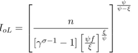
De…ne IoL `o L(j!+ 1) as the potential menace of outsiders, that is the probability of

outsiders’ innovative success in the absence of any bias (i.e. when j! = 0). The Bellman

equation of the leader before its credibility has been acquired can be then written as:

rvL(j!) = L IoLcos j!vL(j!) c ( j!; ) (16)

Proposition 2 When free entry in the research sector holds, there exists an optimal choice of bias if its impact ( ) is high enough. Its value is constant for a constant potential outsider menace (IoL) and is given by

cos = f

IoL

1

(17)

Proof. See Appendix A.1.2.

As expected cos decreases with IoL: A higher potential menace of replacement implies a

more aggressive defensive strategy. Moreover, for a given value of IoL regulation reduces the

bias:17 Recalling that outsiders’ (de facto) probability of R&D success is Io = IoLcos ; one

easily veri…es:

Io= I_oL

f

(18)

This hazard rate converges toward its potential Io ! IoLwhen ! 1. Hence, a high level

of regulation may (asymptotically) eliminate the bias (cos _{! 1).}

In particular, can determine whether the credibility condition holds. For a low enough level of regulation, the bias delivers credibility. In that case the economy jumps to a permanent monopolist framework with an innovative leader whose value is that of equation (15,b). The choice of in this limit case is established by Proposition 3.

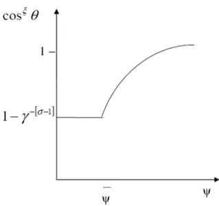
Proposition 3 When the leader credibility is ensured, the optimal value of bias is

cos =h1 [ 1]i (19)

Proof. It follows immediately from (15,b).

Here the incumbent enjoys permanent pro…ts as an innovative monopolist. Once this domi-nant position has been achieved, higher level of bias will only increase costs without additional value. Therefore, the leader does not need further R&D advantages beyond the credibility point. Thus, two type of equilibriums can arise. In the …rst case, outsiders do all R&D and the leader delays its replacement in a Schumpeterian replacement equilibrium (SR). In the second situation, the leader may become the sole innovator enjoying permanent pro…ts in a Permanent monopolistic equilibrium (P M ). To identify the underlying conditions of each type of equilib-rium, the schedule of decisions studied so far needs to be completed with the macro steady-state analysis. This is what the next section does.

2.5 Global accounting and steady state

Given the semi-endogenous nature of the innovation rate, the anlysis here consists in identifying the potential menace of ousiders that underlies the de facto innovation rate at equilibirum. Since this menace trigger the defensive reaction of the leader, whe then analyse how regulation a¤ects the choice of the leader at equilibirum and, thereby, the steady-state equilibrium itself.

2.5.1 The Schumpeterian replacement equilibrium

The macro equilibrium for a continuum Schumpeterian replacement is given by the ful…llment of the labour market clearing and the free entry condition in the research sector. Labour market clearing under full employment needs the addition of labour used in research Lr =

1 R 0 `o(j!+ 1) d!, manufacturing Ly = 1 R 0

L d (j!) d! and defensive activities related to

technolog-ical bias Lf = 1

R

0

c ( ; ) d!. The focus here is the symmetric steady state equilibrium in which

expenditure E and outsiders innovation rate I0 are constant. The latter implies that I0L is also

constant and so cos . Using the de…nition of the average quality index Q introduced in equation (6) and the quality index of each industry (j!+ 1) = [j!+1][ 1], the demand for labour in

Lr=

Io 1

h cos Q (20)

After including demand equation (2), labour required for manufacturing is:

Ly = L

E p

To obtain the labour demand for defensive activities, the de…nition of c ( ; ) in (8) and the

average quality index are used to obtain18:

Lf =

f

h cos Q

The full employment condition requires that L = Ly+ Lr+ Lf , which is equivalent to:

1 = E p + Io 1 h cos Q L + f h cos Q L (21)

To include the free entry, the …rm value of the replacement case (15,a) is substituted on the RHS of (9) and the outsiders’R&D productivity for constant values of IoLand cos on the LHS.

In addition, equation (4) must be veri…ed at E_E = 0 , so that r = :

E = Q L p p 1 + I0 h cos + f h cos (22)

Clearly, in a steady-state equilibrium in which IoL and E are constant, x Q_L must also be

constant. Hence, population and average quality must grow at the same rate:

Q

Q =

L

L = n (23)

Therefore, the model builds on the same tractable properties of a standard semi-endogenous growth model without scale e¤ects.19 The rate of growth of Q is obtained in the usual way. Using the law of large numbers, the variation of average quality is computed by adding the expected technological jump of each industry: Q =

1

R

0

Io[ (j!+ 1) (j!)] d!. After using the

de…nition of Q, this expression reduces to:

1 8

Because industries are symmetric in probabilities, cos (which depends on I0L) can be considered as a

constant inside integrals.

1 9

After putting demands (2) into the instantaneous utility (1), taking logs and di¤erencing, the growth of the average quality implies the standard steady-state utility growth u(t)_u(t)= n₁:

Q Q = Io

1 ₁

In steady state, condition (23) must hold. Thus, the innovation rate is:

Io=

n

[ 1 _1] (24)

Using this result and equation (18), the consequent steady-state potential menace of outsider s is: IoL = 2 6 6 4 n [ 1 _1]h fi 3 7 7 5 (25)

The technological bias in steady-state in the SR equilibrium is obtained by putting (25) into (17), which leads to:

cos = " 1 _{1 f} n # (26) The steady-state level of bias keeps the property of the partial equilibrium decision: when ! 1 the bias vanishes (cos ! 1). By constraining the possibilities of bias, regulation is at the core of the jump from continuous …rm renewal (the SR equilibrium) to a permanent leadership (the P M one). This result is expressed in the following proposition.

Proposition 4 For > there exists a unique level of regulation de…ning the threshold between the Schumpeterian replacement and the permanent monopolist cases involved in the value of the leader …rm (15).

Proof. See Appendix A.1.3.

Figure 2 illustrates the steady-state decision of bias given the value of regulation. For 2 1; the bias is set following equation (19). Thereafter, the leader must take into account free entry of outsiders and decides accordingly to 26).

Figure 2. Leader’s optimal choice of bias

The e¤ect of regulation on R&D e¤ort in steady-state can be analysed through the share of labour allocated to research sr L_Lr. This share can be obtained from the system of equations

(21) and (22) for two unknowns: x Q_L and E . Solving this system for x and using Lr as

expressed by (20) gives: sr= 1 rep+ 1_{[p 1]} p (27) Where rep 1 +[ 1 [ 1]_] [p 1]n + 1

1_{[p 1]}: The following proposition can now be stated.

Proposition 5 In the Schumpeterian equilibrium, regulation ( ) increases the labour share allocated to R&D (sr) and its e¤ ect is all the more important that the size of innovation ( ) is

bigger.

Proof. See Appendix A.1.4.

As R&D becomes harder, at equilibrium, less …rms will be willing to enter the R&D race. The aggregate labour allocated to R&D then decreases. The size of innovation increases mar-ginal revenues as well as the cost of climbing the quality-ladder in the next R&D race. Both Schumpeterian channels combine to modulate the R&D incentives stemming from bias reduc-tions. For p = , the multiplicative factor of in (27) is increasing in : the e¤ect of regulation

2.5.2 The permanent monopolist equilibrium

In a situation with a permanent monopolist, the free entry condition in the research sector no longer holds. Instead, the steady-state equilibrium condition is given by the interest rate (14) that allows a positive and …nite amount of research. In this equilibrium some minor adaptations for labour market clearing must be considered. First, the monopolist allocate labour to research without being a¤ected by the bias. Its probability of innovative success is then IL = `L L.

Second, the optimal choice of bias is now given by cos = 1 [ 1] . Full employment requires: 1 = E p + IL 1 h Q L + f h 1 [ 1] Q L (28)

As before, if expenditure and innovation rates are constant, then Q_Q = L_L = n: Thus the steady-state rate of innovation remains the same: IL= _[ n1 _1].20

Putting the interest rate (14) into the optimal path of expenditure (4) implies:

E = 1 [ 1] _h Q L p p 1 (29)

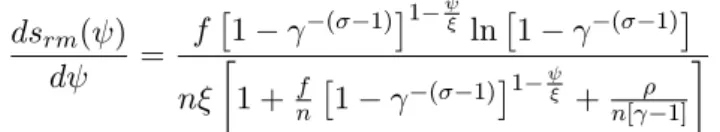
The steady-state share of labour allocated to R&D srm= L_Lr for the permanent monopolistic

case can be obtained by substituting E; as de…ned by (29), into labour market clearing (28) for IL at the steady state. This yields:

srm = 1 " per+ f n[1 ( 1)_] 1 # (30) Where per 1 +_{n[p 1]}.

Proposition 6 In the permanent monopolist equilibrium, regulation ( ) reduces the share of labour allocated to R&D (srm).

Proof. See Appendix A.1.5.

In this equilibrium the monopolist is the innovator. If regulation increases, but not enough to ensure a continuous monopolistic replacement, resources that potentially can by employed in

2 0

Since E is constant, consumption growth is still given byu(t)_u(t)= n 1:

R&D must be allocated for defensive activities. The R&D e¤ort then decreases.

3

Evidence

Accordingly to the model, the reasons to expect a positive correlation between regulation re-strictions and R&D intensity is that they set the boundaries under which the innovative activity is conducted. Within a second best context, rather than limiting the scope for innovative im-provements these rules may act as a market coordination device able to deliver standardisation and knowledge di¤usion. This coordination may probably be a de facto consequence of some practices usually seen as market barriers. This section empirically analyses this possibility at the industry level.

3.1 Empirical strategy

Industry-level data has the advantage of exploiting heterogeneity in R&D e¤ort coming from di¤erent competitive environments. It also captures phenomenons that are aggregate in nature, similar to those analysed in the model. However, as it well is the case with most micro data sets, information on potential entrants (outsiders) is not available. Therefore, it is not possible to analyse in detail the conditions under which the SR and the P M equilibrium arise. Some practical guidelines must be assumed in order to link the model with the data.

Notice that the outcome of zero R&D e¤ort comes from the choice of CRS in R&D, the standard assumption used for tractability. In practice, monopolists are replaced, even if they remain for a long period of time. Consequently, the empirical exercise starts assuming that, in average, industries are mainly concerned with the Schumpeterian equilibrium (sections 3.3.2 and 3.3.3). Section 3.3.4 then moves one step forward in identi…cation and study how these results change when low- and high-regulation environments are analysed separately.

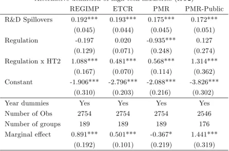
High-technology industries (HT) are assumed to make bigger innovative steps than the rest of industries. They are de…ned as 30-33 ISIC Rev-3 industries. This includes the information and communication technologies (ICT industries) and the manufacturing of medical precision and optical instruments. The robustness check section (3.3.2) tests an alternative de…nition including industries 29 (machinery and equipment) and 34 (motor vehicles ), usually seen as using intensely ICT technologies. It is expected that the kind of innovation of HT industries allows for relatively high monopolistic incentives. If this is true and if in average industries are in a Schumpeterian equilibrium, the R&D incentives induced by regulation should be higher in

HT.

Let yit be the measure of aggregate R&D e¤ort (labour share in the model) of industry i at

time t. Denoting ritthe regulation proxy and HT the dummy variable identifying HT industries,

the following equation is estimated:

yit= 1 rit+ 2 rit HT + 3 HT + 5xit+ it (31)

where it = i+ it , xit is a vector of controls (see section 3.2.2) and all continuous variables

are in natural logs. Under this speci…cation, the marginal e¤ect of regulation can be computed as

@E [yitjHT ]

@Rit

= 1 + 2 HT

If HT = 0 then the marginal e¤ect is 1 and re‡ects the e¤ect of regulation on non-HT

industries. When HT = 1 the marginal e¤ect is 1 + 2 : This means that 1 is also the

e¤ect of regulation which is common to HT and non-HT industries. Hence, 2 is the e¤ect of

regulation on R&D intensity in HT industries relative to non-HT ones.

The Schumpeterian equilibrium predicts a positive e¤ect of regulation on R&D intensity that increases with the size of innovation. Using the full sample, a positive and signi…cant estimate_b2

is expected. In other words, if an R&D-boosting e¤ect of regulation can be expected following the model, it is more likely to be observed in the speci…city of high technology industries. In absolute terms, the over all e¤ect of regulation on R&D intensity in HT industries will be given by b1 +b2. While the signi…cance of b2 can be obtained directly from the regressions,

for _b1 + b2 the joint signi…cance p b1+b2

b_{b1 b1}+b_{b2 b2}+2b_{b1 b2} is required, where bab is the sample

covariance between a and b.

It is probable that a …xed component in the error term is associated to each country-industry couple. The bias produced by this unobserved time-invariant heterogeneity can be eliminated by a within-group estimator, but at the cost of losing the information provided by _b3. When

substracting the sample mean of each variable by group, the transformation of the within-group estimator eliminate _i, but also all time-invariant variables such as HT . However, the …xed e¤ect will contain the dummy HT; so that the estimates of _b2 and b1+b2 should remain consistent.

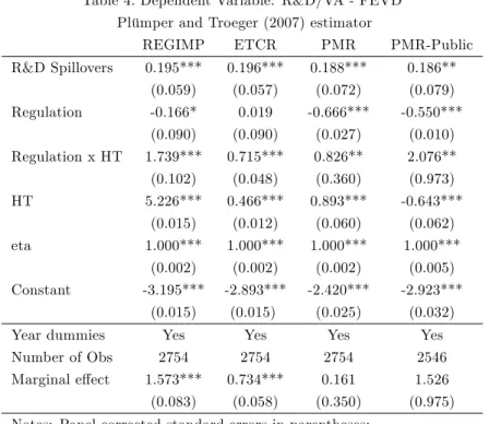
In the robustness checks, use is made of the three-steps …xed-e¤ect decomposition proposed by Plümper and Troeger (2007) that helps to handle this type of time-invariant variable when there

are reasons to suspect individual unobserved heterogeneity.

3.2 Data

3.2.1 R&D and regulation

The data set contains information for 14 manufacturing industries across 14 OECD countries for the period 1987-2003. R&D series are provided by the OECD ANBERD dataset. The sample period is mainly limited by R&D data availability. The dependant variable, R&D intensity, is measured as R&D expenditure over value added. The latter series were obtained from the 60-Industry database of the Groningen Growth and Development Centre (GGDC).21 Appendix (A.2) gives a summary of the sample.

Indicators of regulation are computed by the OECD.22 _{Their attractiveness is that they}

rely on administrative practices that are usually seen as market barriers. These practices are collected and coded for speci…c areas of regulation and give the basis to compute what the OECD calls low-level indicators. To construct aggregate indicators, a bottom-up approach is implemented using weights that seek to re‡ect information availability and the nested structure of the areas included in the aggregate indicator. Four global indicators of regulation are used.

The economy-wide indicator of product market regulation (henceforth PMR): It is com-posed of a collection of inward- and outward-oriented indicators of market barriers re‡ect-ing state control, barriers to entrepreneurship and barriers to trade and investment a the national level. While close to regulatory practices its availability in time dimension is a drawback. It is only available for 1998 and 2003 and has been consequently distributed into the sample before and after 2000.23

The Size and scope of the public enterprise sector (henceforth PMR-Public): It is an important low-level component of PMR that captures the degree of active participation of the state in product markets. One can expect that R&D activities and …rm operation where the State is strongly active are more restricted.

The indicator of network sectors (henceforth ETCR): It is an indicator of regulation in seven sectors related to energy, transport and communication (telecoms, electricity, gas,

2 1

http://www.ggdc.net/databases/60_industry.htm

2 2_{www.oecd.org/eco/pmr} 2 3

This arbitrary distribution seeks to re‡ect the timing of surveys and, under a …xed-e¤ect speci…cation, it should have minor consequences on estimations.

post, rail, air passenger transport, and road freight). It is available in times-series at the country level and focuses on areas such as barriers to entry, public ownership, market structure and price controls. As network sectors have been one of the main target of wider deregulation policies, they help to capture the evolution of the competitive environment at the national level.

The impact of service regulation on manufacturing (henceforth REGIMP): It captures the "knock-on" e¤ects associated to regulation in (i) network services; (ii) retail distribution and professional business services (RBSR) and (iii) …nance. Information on regulation in retail and business services deals with barriers to entry, price controls and constrains on business operations for 1998 and 2003. Regulation on the …nancial sector stems from De Serres et al. (2006) who provide regulatory practices on the banking system and …nancial instruments in the period 2002-2003. The projection of regulation of services sectors on manufacturing industries is made accordingly to input/output matrices informing about the use of these sectors as intermediates inputs. The main advantage of this indicator is that it is available in the form of time-series cross-section data.

The details of the methodology, questionary and construction of PMR can be found in Conway et al. (2005). The methodology and analysis related to REGIMP and ETCR is fully documented in Conway and Nicoletti (2006). While REGIMP and ETCR are more indirect measures of product market competition, they remain highly correlated to the PMR aggregate indicator (78% and 64%, respectively) and have the advantage of providing information in time series. For these reasons they will be emphasised in the presentation of the empirical results, specially REGIMP which presents a pseudo-panel variability compatible with that of the explained variable.

An important question is the extent to which these indicators re‡ect the kind of regulation described in the model. In the theoretical setting regulation is seen as a device constraining the way in which the new discovery is introduced into the market. While the OECD indicators are constructed with the aim of capturing practices supposed to curb competition, by de…nition, they measure barriers that limit the action of actors. In this sense, REGIMP has the advantage of capturing the restrictions induced by utility sectors (network services, retail, business services and …nance) on the provision and fabrication of manufactured goods. Domestic regulation in these sectors will particularly shape entry and operation in manufacturing industries as they represent key inputs, mainly produced by natural monopolies where import penetration plays a

minor rôle. For instance, some of the practices considered by the indicators of regulation in retail and professional services include limitations such as licensing permits, restrictions on entrepre-neurial choices and on the type of products that can be o¤ered (see Conway and Nicoletti, 2006 Appendix). Firms that use theses services will be probably constrained in their implementation of new business solutions. Similarly, restrictions on the furniture of communication, transports and energy will clearly delimit the way to introduce new goods on the market.24

3.2.2 Other explanatory variables

In order to control for alternative determinants of R&D intensity, the following variables are considered:

R&D spillovers: as stressed by several works in endogenous growth, controlling for the innovative e¤ort performed at the world level, helps to take into account the knowledge externalities as well as the possible strategic complementarity in R&D investments. For each country, industry and period these externalities are proxied by the R&D intensity performed by the rest of countries in the same industry. As they vary in both cross-section and time dimension, R&D spillovers are a good indicator of the evolution of the international technological context of each individual (country-industry couple).

Proximity to the technology frontier: The technology gap of the industry vis-à-vis the world technology frontier can be an important determinant of innovation and, as such, of the innovative underlying e¤ort. Industries competing close to the frontier may require more adaptation to technological change and so more innovative e¤ort than laggards ones. For a given period, the proximity to the technology frontier is measured as the labour productivity of each country-industry couple relative to the highest one observed at the world level in the same industry. In order to provide a more accurately identi…cation of the most productive industry, the transversal de‡ation of value-added uses PPAs at the industry level, provided by Timmer et al. (2007) for 1997.

Capital intensity: Capital can be correlated to R&D e¤ort by several channels. While it can render search routines more e¢ cient it can also be a substitute in the case of industries that heavily rely on embodied technical change. On the other hand, because of

2 4_{Conway and Nicoletti (2006) report that in the late 1990 roughly 80% of the output of business services was}

used as intermediate in other sectors of the economy and that …nance, electricity, post and telecommunication sectors accounted represented between 50%-70% of intermediate inputs in production processes.

complementarities between high-skills and capital, these indicator may indirectly correct for potential bias induced by the omission of variables related to human capital endowment Capital intensity is computed as the ratio of de‡ated capital stock (from OECD STAN) to hours worked (GGDC). Capital stock has been obtained from cumulative investments thanks to a perpetual-inventory rule using a 7% depreciation rate. The main drawback of these series is the lack of availability of information for some countries, which translates into a reduction of roughly half of the sample. Related results should be then analysed with caution.

Financial deepness: It is included since innovation can be constrained not by the lack of incentives but by …nancial market imperfections. Financial development is proxied by the ratio of total asset investment of institutional investors over GDP available from the OECD (Institutional Investor database).

3.3 Results

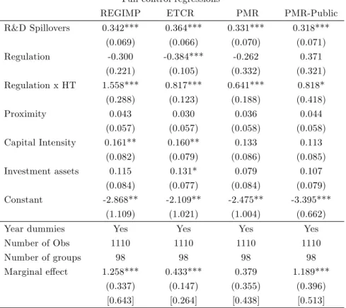
3.3.1 A di¤erentiated impact of regulation depending on the technological level Table 1 reports the main results using the full sample. Within-group regressions are presented considering Huber-White corrected standard errors. The impact of R&D spillovers (R&D in-tensity of the rest of the world in the same industry) on R&D inin-tensity is signi…cantly positive in all speci…cations. Indeed, this correlation appears in most of regressions. Column [1] and [2] presents regressions using the "knock-on" e¤ect of non-manufacturing regulation on manu-facturing activities, captured by the regulation proxy REGIMP. It represents the widest source of variance as it is available in time-series cross-section data. Following REGIMP, regulation does not account for a signi…cant e¤ect on R&D intensity in non-HT industries . However, in line with what can be deduced from the model’s prediction, one observes a positive e¤ect of regulation which is speci…c to HT industries. This is true in relative and absolute terms. In relative terms this result is given by the positive and signi…cant coe¢ cient of the interaction between REGIMP and the dummy variable de…ning high-tech industries. In absolute terms, this positive correlation is shown by the marginal e¤ect (ME) computed in the bottom part of Table 1. As explained above, this ME considers both (a) the e¤ect of regulation that is common to HT and non-HT industries (_b1 in equation 31) and (b) the e¤ect of regulation that is speci…c

to HT industries (_b2 in equation 31). It could be argued that the data structure might imply

of standard errors and clustering at the industry level. The table reports the clustered standard errors for the marginal e¤ect in squared brackets. One easily veri…es that the signi…cance of the ME is still preserved at conventional levels under this heteroskedasticity robustness check.

These results are con…rmed by the regulation proxy ETCR (columns [3] and [4]) that mea-sures regulatory provisions in network sectors. As suggested by (Conway and Nicoletti, 2006), this indicator mirrors the trend of regulatory reforms at the national level.25 Interestingly, here, in the basic model of column [3], regulation presents a signi…cantly positive correlation with R&D intensity. As before, one the interaction is included, a di¤erentiated e¤ect appears. Both the interaction term and the ME suggest a positive impact of regulation on HT industries. This is also robust to the clustered correction of the standard errors.

Results are slightly di¤erent for the product market regulation proxy PMR (columns [5] and [6]). PMR is an aggregate of economy-wide indicators aiming at capture market barriers. It does not vary in every period. Two points in time are available. This is probably the main reason for some changes in the estimations. Now, in the simple model (column [5]) regulation appear to be negatively associated to R&D. This is also true for the e¤ect of regulation in non-HT technologies in column [6]. In this regression, a positive and signi…cant interaction between regulation and HT industries shows up. Hence, PMR regressions illustrate more sharply the di¤erentiated e¤ect of regulation depending on the technological level. The sum of the positive R&D e¤ect of regulation in HT industries and the negative one, common to all industries, yields a non signi…cant overall ME.

The last two columns focus, among market barriers summarised in PMR, on the size and the scope of the public sector (PMR-Public). One should expect that a higher and active state imposes higher regulation, namely in the production of new varieties. As in the case of ETCR, the e¤ect of regulation in the simple model is again positive and signi…cant for PMR-Public (column [7]). The di¤erentiated e¤ect of regulation is also suggested here. Namely, one observes a positive correlation between regulation and R&D e¤ort in HT industries. This time, contrary to the aggregate PMR indicator, this also true in absolute terms and robust to clustering.

Overall these results based on the full sample are in line with the main model’s prediction regarding the Schumpeterian equilibrium. As regulation increases, the dissuasive e¤ect of de-fensive strategies can be reduced. R&D incentives are higher, but the …nal impact of regulation

2 5

Usual rankings of regulation at the national level are quite in line with the picture generated by this indicator. For instance, in average in our sample, Greece and Italy appear as the most regulated countries. UK and US on the contrary are in the opposite extreme.

is modulated by the size of innovation since it shapes monopolist incentives. This prediction implies that the positive e¤ect of regulation should empirically be found when the size of inno-vation is higher. This is con…rmed by the estimates of the interaction term in all regressions and by the overall marginal e¤ect in almost all of them, namely in those using the most e¢ cient proxies of regulation.

T a b le 1 . D ep en d en t V a ri a b le : R & D / V A -W it h in -g ro u p es ti m a te s B a si c co n tr o l re g re ss io n s R E G IM P E T C R P M R P M R -P u b li c [1 ] [2 ] [3 ] [4 ] [5 ] [6 ] [7 ] [8 ] R & D S p il lo v er s 0 .1 4 6 * * * 0 .1 9 5 * * * 0 .1 3 4 * * * 0 .1 9 6 * * * 0 .1 4 0 * * * 0 .1 8 8 * * * 0 .1 4 2 * * * 0 .1 8 6 * * * (0 .0 4 6 ) (0 .0 4 2 ) (0 .0 4 5 ) (0 .0 4 0 ) (0 .0 4 6 ) (0 .0 4 4 ) (0 .0 5 1 ) (0 .0 5 0 ) R eg u la ti o n 0 .0 0 1 -0 .1 6 6 0 .2 5 4 * * * 0 .0 1 9 -0 .7 2 7 * * * -0 .9 0 8 * * * 0 .6 6 3 * * * 0 .1 3 0 (0 .1 2 7 ) (0 .1 2 5 ) (0 .0 8 2 ) (0 .0 6 8 ) (0 .2 3 3 ) (0 .2 4 0 ) (0 .2 3 4 ) (0 .2 4 5 ) R eg u la ti o n x H T 1 .7 3 9 * * * 0 .7 1 5 * * * 0 .8 2 6 * * * 2 .0 7 6 * * * (0 .2 2 5 ) (0 .0 8 8 ) (0 .1 4 4 ) (0 .4 6 1 ) C o n st a n t -2 .6 1 0 * * * -1 .7 8 9 * * * -3 .0 4 8 * * * -2 .7 6 8 * * * -2 .1 9 2 * * * -2 .0 5 0 * * * -3 .9 1 3 * * * -3 .7 9 7 * * * (0 .5 3 7 ) (0 .6 2 8 ) (0 .4 2 0 ) (0 .3 5 3 ) (0 .2 1 5 ) (0 .3 8 5 ) (0 .3 0 7 ) (0 .2 9 3 ) Y ea r d u m m ie s Y es Y es Y es Y es Y es Y es Y es Y es N u m b er o f O b s 2 7 5 4 2 7 5 4 2 7 5 4 2 7 5 4 2 7 5 4 2 7 5 4 2 5 4 6 2 5 4 6 N u m b er o f g ro u p s 1 8 9 1 8 9 1 8 9 1 8 9 1 8 9 1 8 9 1 7 6 1 7 6 M a rg in a l e¤ ec t 1 .5 7 3 * * * 0 .7 3 4 * * * -0 .0 8 2 2 .2 0 6 * * * (0 .2 5 6 ) (0 .1 1 7 ) (0 .2 2 6 ) (0 .4 3 8 ) [0 .5 9 7 ] [0 .3 0 0 ] [0 .3 8 4 ] [0 .7 6 9 ][ N o te s: H u b er t-W h it e co rr ec te d st a n d a rd er ro rs in ro u n d p a re n th es es a n d cl u st er ed a t th e in d u st ry le v el in sq u a re d b ra ck et s; * , * * ,* * * d en o te si g n i… ca n ce a t 1 0 % , 5 % a n d 1 % , re sp ec ti v el y