HAL Id: hal-03096777
https://hal.archives-ouvertes.fr/hal-03096777
Submitted on 6 Jan 2021
HAL is a multi-disciplinary open access
archive for the deposit and dissemination of
sci-entific research documents, whether they are
pub-lished or not. The documents may come from
teaching and research institutions in France or
abroad, or from public or private research centers.
L’archive ouverte pluridisciplinaire HAL, est
destinée au dépôt et à la diffusion de documents
scientifiques de niveau recherche, publiés ou non,
émanant des établissements d’enseignement et de
recherche français ou étrangers, des laboratoires
publics ou privés.
of CFC-11, CO2, and ∆14C
Z. Lachkar, J. Orr, J.-C. Dutay, P. Delecluse
To cite this version:
Z. Lachkar, J. Orr, J.-C. Dutay, P. Delecluse. Effects of mesoscale eddies on global ocean distributions
of CFC-11, CO2, and ∆14C. Ocean Science, European Geosciences Union, 2007, 3 (4), pp.461-482.
�10.5194/os-3-461-2007�. �hal-03096777�
www.ocean-sci.net/3/461/2007/
© Author(s) 2007. This work is licensed under a Creative Commons License.
Ocean Science
Effects of mesoscale eddies on global ocean distributions of CFC-11,
CO
2
, and 1
14
C
Z. Lachkar1,*, J. C. Orr2, J.-C. Dutay1, and P. Delecluse1,**
1LSCE/IPSL, Laboratoire des Sciences du Climat et de l’Environnement, CEA-CNRS-UVSQ, Gif-sur-Yvette, France 2Marine Environment Laboratories, International Atomic Energy Agency, Monaco
*now at: Institute of Biogeochemistry and Pollutant Dynamics, ETH Zurich, Zurich, Switzerland **now at: Centre National de Recherches M´et´eorologiques, Meteo-France, Paris, France
Received: 19 June 2006 – Published in Ocean Sci. Discuss.: 31 July 2006 Revised: 17 July 2007 – Accepted: 4 October 2007 – Published: 12 October 2007
Abstract. Global-scale tracer simulations are typically
made at coarse resolution without explicitly modelling ed-dies. Here we ask what role do eddies play in ocean up-take, storage, and meridional transport of transient trac-ers. We made global anthropogenic transient-tracer simula-tions in coarse-resolution (2◦cos ϕ×2◦, ORCA2) and eddy-permitting (12◦cos ϕ×12◦, ORCA05) versions of the ocean general circulation model OPA9. Our focus is on surface-to-intermediate waters of the southern extratropics where air-sea tracer fluxes, tracer storage, and meridional tracer transport are largest. Eddies have little effect on global and regional bomb 114C uptake and storage. Yet for anthro-pogenic CO2and CFC-11, refining the horizontal resolution
reduced southern extratropical uptake by 25% and 28%, re-spectively. There is a similar decrease in corresponding in-ventories, which yields better agreement with observations. With higher resolution, eddies strengthen upper ocean verti-cal stratification and reduce excessive ventilation of interme-diate waters by 20% between 60◦S and 40◦S. By weakening
the residual circulation, i.e., the sum of Eulerian mean flow and the opposed eddy-induced flow, eddies reduce the supply of tracer-impoverished deep waters to the surface near the Antarctic divergence, thus reducing the air-sea tracer flux. Thus in the eddy permitting model, surface waters in that region have more time to equilibrate with the atmosphere before they are transported northward and subducted. As a result, the eddy permitting model’s inventories of CFC-11 and anthropogenic CO2are lower in that region because
mixed-layer concentrations of both tracers equilibrate with the atmosphere on relatively short time scales (15 days and 6 months, respectively); conversely, bomb 114C’s air-sea equi-libration time of 6 years is so slow that, even in the eddy per-mitting model, there is little time for surface concentrations
Correspondence to: Z. Lachkar
(zouhair.lachkar@env.ethz.ch)
to equilibrate with the atmosphere, i.e., before surface waters are subducted.
1 Introduction
The ocean’s large capacity to take up and store carbon me-diates the increase of anthropogenic CO2in the atmosphere.
Thus, accurately determining ocean uptake of anthropogenic tracers is relevant not only to understanding the global car-bon cycle, but also to predicting the magnitude of future cli-mate change. Ocean models have been used extensively to understand air-sea fluxes and ocean storage of anthropogenic carbon. Storage of anthropogenic carbon has also been es-timated with data-based approaches (Gruber et al., 1996; Sabine et al., 2004), but these are not without substantial ran-dom and systematic errors (Matsumoto and Gruber, 2005).
During the last decade, the Ocean Carbon-Cycle Model Intercomparison Project (OCMIP) examined and compared several existing ocean general circulation model (OGCM) simulations of transient tracers (Orr et al., 2001; Dutay et al., 2002; Watson and Orr, 2003; Matsumoto et al., 2004). All the OCMIP models used a coarse-horizontal grid and re-sorted to parameterising the effect of unresolved subgrid mixing processes on larger scales. The OCMIP models dis-agree substantially in terms of the simulated anthropogenic CO2 air-sea flux within the southern extratropics (the
re-gion south of 20◦S), which absorbs up to half of the global
oceanic uptake (Orr et al., 2001; Watson and Orr, 2003). More recently, Matsumoto et al. (2004) compared simulated natural radiocarbon, anthropogenic CO2, and CFC-11 from
19 ocean carbon cycle models with data-based estimates and also found large discrepancies between model results. These model discrepancies are partly associated with differences in the representation of subgrid-scale ocean mixing processes
(Matear, 2001; Dutay et al., 2002). In the only attempt to date to use a global eddy resolving model (1/10◦) to simulate
the ocean CFC-11 distribution, Sasai et al. (2004) demon-strated much improved agreement with the observations in the southern extratropics. In particular, their model exhibits improved skill south of 40◦S with none of the excessive ventilation of thermocline and intermediate waters that is characteristic of most of the OCMIP coarse-resolution mod-els. Thus, generally improving the ability to account for mesoscale eddies may be key to correctly simulating the up-take, transport, and storage of the transient tracers, especially in southern extratropics. To improve eddy parameterisations for coarse-resolution models, ocean modellers can learn from how ocean eddies affect global and regional ocean tracer bud-gets.
During the past three decades, physical oceanographers have made significant advances in discerning the role that ed-dies play in the ocean’s general circulation (Holland and Lin, 1975a,b; Holland, 1978). Cox (1985) investigated the effects of mesoscale eddies within the subtropical thermocline and highlighted the eddy-induced homogenisation of anomalous Potential Vorticity along isopycnals. In terms of meridional heat transport, B¨oning and Budich (1992) found a negligi-ble effect of eddies when using a primitive equation model for an idealised ocean basin. Drijfhout (1994) showed that the eddy-induced mean meridional circulation nearly com-pensates poleward eddy heat transport for the case of a weak diabatic forcing. Vallis (2000) demonstrated how mesoscale eddies could be important in determining ocean stratification. Marshall et al. (2002) and Marshall and Radko (2003) used idealised simulations for a channel-only domain, finding that eddies help to set both the stratification and the depth of the permanent thermocline in the ocean.
Despite these advances, all studies have been limited by the compromises that must be made because of the computer-intensive nature of making simulations that in-clude mesoscale variability in global-scale numerical mod-els. Previous work has generally used simplified basin-scale models to investigate the genesis of mesoscale eddies and their interaction with the mean flow. Few studies indeed have addressed how ocean eddies may affect global-scale trans-port and distribution of transient tracers. Here we attempt to elucidate the importance of mesoscale eddies in terms of their effect on the global distributions of transient tracers. To isolate the effect of eddies, we follow the lead of Cox (1985) and Thompson et al. (1997), who compared integra-tions of a noneddying and an eddying versions of the same model. Thus we also compare a coarse-resolution to an eddy-permitting version of the same OGCM.
In addition to anthropogenic CO2, we also made
simula-tions of CFC-11 and bomb 114C to better evaluate model performance and to investigate how mesoscale eddies affect transient tracers with different air-sea equilibration times. That is, these three tracers require different times for their mixed-layer concentrations to equilibrate with the
atmo-sphere. For a purely inert tracer, the equilibration time τeq
can be estimated following Broecker and Peng (1974) as
τeq=hv where h is the mixed-layer depth and v the tracer
piston velocity. Between 60◦S and 40◦S, the air-sea equi-libration time for typical gaseous tracers, including CFC-11, is ∼14 days, whereas for bomb 114C it is ∼6 years. Lying between these two extremes is the anthropogenic CO2’s
air-sea equilibration time of ∼6 months. Equilibration for CO2
is slower than for CFC-11 because when added to seawater, CO2does not remain a dissolved gas as does CFC-11;
in-stead, it reacts with carbonate ion CO2−3 to form bicarbonate ion HCO−3. What matters then is the change in the mixed-layer concentration of the sum of these three species (i.e., dissolved inorganic carbon DIC), not just the change in CO2
concentration. Relative to CFC-11, the time for a perturba-tion in mixed-layer DIC to equilibrate with the atmosphere is longer by a factor of ∂[∂[CODIC]
2∗] (Sarmiento and Gruber, 2006).
That factor averages 12 between 60◦S and 40◦S whereas it averages 19 globally, based on the GLODAP data. For bomb
114C, the equilibration time between the mixed layer and the atmosphere is much longer still because isotopic equilibrium requires that CO2exchange its isotopic composition with the
entire DIC pool. The corresponding factor is then [[CODIC]
2∗],
which averages 140 between 60◦S and 40◦S and 180 glob-ally.
The air-sea equilibration time has already been shown to affect transport and uptake of transient tracers in an idealised model of the Southern Ocean (Ito et al., 2004). Here we aim to use an OGCM to evaluate the effects of mesoscale eddies on large-scale uptake, storage, and meridional trans-port of CFC-11, anthropogenic CO2, and bomb 114C, while
focusing particularly on the southern extratropics where up-take and storage are largest. We also aim to investigate how mesoscale eddies alter ocean dynamics in the higher south-ern latitudes and to examine the mechanisms by which they affect large-scale distributions of transient tracers.
2 Methods
2.1 Strategy
We made a series of simulations for CFC-11, anthropogenic CO2 and bomb 114C, using a noneddying version of the
model having a 2◦cos ϕ×2◦ coarse-grid (termed ORCA2), where ϕ is latitude. We also made analogous simula-tions with an eddying version of the same model using a
1 2
◦cos ϕ×1 2
◦grid (ORCA05), whose grid size is 34 km on
average, globally, and is 28 km at 60◦S. The eddying version of the model has sufficient horizontal resolution to resolve the largest mesoscale eddies (those with diameter larger than two or three times the grid size), although it does not resolve the rest of the mesoscale eddy spectrum. For comparison, to be fully “eddy-resolving” there would need to be at least 12 grid points per wavelength (Chassignet and Verron, 2006),
i.e., a grid size at least six times smaller than the first Rossby Radius of deformation, which varies between 10 and 20 km in high latitudes (Chelton et al., 1998). The main goal of this work is to explore how simulated ocean uptake of transient tracers changes as one begins to explicitly resolve mesoscale eddies, i.e., when moving from a coarse-resolution to an eddy-permitting OGCM. We will address if crossing that threshold is important in terms of transient tracer uptake, al-though studying the effects of moving to finer resolution is beyond the scope of this study.
Although the eddying model does not resolve the en-tire spectrum of mesoscale eddies, it does exhibit substan-tial eddy activity in the Southern Ocean along some of the most energetic currents in the world (Fig. 1); conversely, the coarse-resolution model exhibits no such activity. In a first series of two simulations at eddying and noneddying resolu-tion, we deliberately avoided using any subgrid-scale eddy parameterisation in order to better capture the effect of re-solving mesoscale eddies that goes along with an increase in horizontal resolution. Additionally, in order to assess the ef-fectiveness of the most widely used eddy parameterisation, known as GM (Gent and McWilliams, 1990; Gent et al., 1995), to represent the role of mesoscale eddies in ocean up-take of transient tracers, we made two other CFC-11 simula-tions using this parameterisation at both resolusimula-tions. The GM coefficients of thickness diffusivity and isopycnal diffusivity in both simulations were set to 103m2s−1.
Integrating long global carbon simulations until near-steady state requires running the model for several thou-sand years. At eddy-permitting resolution, that would ex-tend far beyond presently available computing resources. To overcome this technical limitation, we used perturbation ap-proaches for both anthropogenic CO2 and bomb 114C. In
so doing, we assume that the natural ocean carbon cycle is not affected directly by the anthropogenic perturbation. Thus we treat anthropogenic CO2and bomb 114C as passive
trac-ers excluding any possible response of the ocean biological process to the anthropogenic CO2 increase. This approach
was introduced for anthropogenic CO2 by Siegenthaler and
Joos (1992) and first used in a 3-D model by Sarmiento et al. (1992). Here we extend it to bomb 114C. Simulations of an-thropogenic CO2begin on 1 January 1765 and are run until
1 January 2000 (industrial era); simulations for bomb 114C start on 1 July 1954 and run until 1 January 2000 (nuclear era).
Despite the advantage of using a perturbation approach, realising online global tracer simulations in an eddying, global-scale OGCM remains a challenge because of the computational requirements. For example, a 235-year an-thropogenic CO2simulation (1765–2000) with our eddying
model requires 11 000 CPU-hours on one processor of a NEC-SX6 vectorial supercomputer. To further reduce com-putational costs we used the offline approach for our tracer simulations. An offline model driven by monthly fields from an (online) eddy-permitting OGCM (0.4◦cos ϕ×0.4◦) was
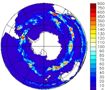
Fig. 1. Surface-ocean eddy kinetic energy in the southern
extrat-ropics (in cm2s−2) of the eddying simulation.
used by Sen Gupta and England (2004) to investigate venti-lation of globally prominent water masses. Hill et al. (2004) used a 1/6◦ North Atlantic regional model, finding that of-fline simulations remain faithful to online runs when the time-averaged flow fields are updated on a timescale close to the inertial period (about 1 day). Here, small eddies associ-ated with high frequency time variability (close to the inertial period) are not present in the flow given that we resolve only the upper range of mesoscale spectrum. Thus we used a 5-day forcing frequency for both eddying and noneddying sim-ulations. With the noneddying version of our model, the of-fline transient-tracer results closely resemble those obtained with the online version, e.g., with zonal means of the inven-tory differing at most by 3%.
To evaluate simulations, we compared simulated to ob-served tracer distributions along vertical sections from the World Ocean Circulation Experiment (WOCE) and to grid-ded data products from Global Ocean Data Analysis Project (GLODAP). The GLODAP data consists of synthesised products from WOCE, the Joint Global Ocean Flux Study (JGOFS), and the Ocean Atmosphere Carbon Exchange Study (OACES) (Key et al., 2004).
2.2 Models
Our simulations were made with the ORCA-LIM global cou-pled ocean-sea ice model whose ocean component is based on version 9 of the model OPA (Oc´ean PArall´elis´e, referred to as OPA9). OPA is a finite difference OGCM with a free surface and a nonlinear equation of state following the Jack-ett and McDougall (1995) formulation (Madec and Imbard, 1996; Madec et al., 1998); The model has a contorted hori-zontal curvilinear mesh in order to overcome the North Pole
singularity found in conventional grids. To avoid the typi-cal northern singularity over the ocean, the OPA9 grid has two poles, one over Canada and the other over Asia, which allows for longer timesteps while still respecting the CFL sta-bility criterion. Variables are distributed on C grid (Arakawa, 1972) on prescribed z-levels. The horizontal grid is also or-thogonal and retains numerical accuracy to the second order (Marti et al., 1992). The model is implemented on a Merca-tor grid, i.e., becoming finer at high latitudes following the cosine of latitude. With 46 levels in the vertical direction, the vertical grid spacing increases from 6 m at the surface to 250 m at the bottom. The bottom of the deepest level reaches 5750 m. Lateral tracer mixing occurs along isopycnal sur-faces via Laplacian diffusion. For the noneddying model, we used horizontal Laplacian diffusion operator, as is typical for coarse-resolution models. For the eddying model, we used the biharmonic formulation for viscosity, in order to make optimal use of the resolved scales and to allow the eddy-ing flow to exhibit its dominant nondiffusive nature (Griffies and Hallberg, 2000). The biharmonic diffusion operator has no advantage at coarse resolution but is much better suited for eddying models because it acts on smaller scales, admit-ting shorter wavelength structures on the mesh that would be damped out by the Laplacian operator (Griffies et al., 2000). Vertical eddy diffusivity and viscosity coefficients are given by a second-order closure scheme based on a prognos-tic equation for turbulent kineprognos-tic energy (TKE) (Gaspar et al., 1990; Blanke and Delecluse, 1993) and are enhanced in the case of static instability. This TKE parametrisation improves simulated equatorial dynamics and the thermocline in a high resolution model (Blanke and Delecluse, 1993). To advect temperature and salinity, we used the Total Variance Dimin-ishing (TVD) advection scheme following L´evy et al. (2001). The bathymetry is calculated using the 20 bathymetry file ETOPO2 from NGDC (National Geophysical Data Center) (Smith and Sandwell, 1997; Jakobsson et al., 2000), except for the zone south of 72◦S where it was computed from the BEDMAP data (Lythe and Vaughan, 2001). The OGCM out-put was stored as 5-day averages to avoid aliasing of high-frequency processes (Crosnier et al., 2001). Initial conditions for the temperature and salinity fields were taken from Levi-tus et al. (1998) for the low and middle latitudes and from the PHC2.1 climatology (Steele et al., 2001) for high latitudes.
The model was started from rest, then spun up for 8 years with a climatological seasonal forcing with daily frequency as computed from the 1992–2000 NCEP/NCAR 10-m wind stress and 2-m air temperature data (Kalnay et al., 1996). Additionally, we used monthly climatologies of precipitation (Xie and Arkin, 1996), relative humidity (Trenberth et al., 1989), and total cloud cover (Berliand and Strokina, 1980). Surface heat fluxes and freshwater flux for ocean and sea-ice were calculated using the empirical bulk parameterisation proposed by Goose (1997).
The sea ice component of ORCA-LIM is the Louvain-la-Neuve sea ice model (LIM), a dynamic-thermodynamic
model specifically designed for climate studies. A full de-scription of LIM is given by Fichefet and Maqueda (1997).
To study passive tracers, we used a tracer-transport (of-fline) version of OPA (OPA Tracer 8.5) driven by 5-day av-erages of fields of advection and vertical turbulent diffusion from the dynamic (online) model. As for active tracers (tem-perature and salinity), we used isopycnal Laplacian mixing with the same lateral diffusion coefficients as in the dynamic model. We employed the flux-corrected-transport advection scheme from Smolarkiewicz (1982, 1983); Smolarkiewicz and Clark (1986). This advection scheme is little diffusive and is positive definite, i.e., it ensures positive tracer concen-trations.
2.3 Passive tracer boundary conditions
2.3.1 CFC-11
CFC-11 (chlorofluorocarbon-11) is a purely anthropogenic trace gas, whose atmospheric concentration has increased from zero since the 1930s. Once it enters the surface ocean via gas exchange, CFC-11 is chemically and biologically in-ert. Thus it serves as a passive conservative tracer and tracks circulation and mixing processes that occur over decadal timescales (Wallace and Lazier, 1988; Doney and Bullister, 1992; Waugh et al., 2003). The large database of oceanic concentrations of CFC-11 come from direct measurements made at ∼1% precision during the World Ocean Circula-tion Experiment (WOCE). Putting that high precision into context, the other two transient tracers can only be esti-mated indirectly from other data, which means errors are relatively much larger and unfortunately difficult to quantify (Matsumoto and Gruber, 2005; Key et al., 2004). To model CFC-11 ocean uptake, we followed the protocols defined by OCMIP-2 (Dutay et al., 2002). That is, passive tracer fluxes at the air-sea interface were calculated according to the clas-sical formulation of air-sea gas exchange
FCFC =KCFC(pCFC−
Cs
αCFC
)(1−I ) (1)
where KCFC is the CFC-11 gas transfer coefficient
(mol m−2yr−1µatm−1), pCFC is the partial pressure of CFC-11 from the reconstructed atmospheric history (Walker et al., 2000), and Cs is the modelled sea surface tracer
con-centration. The αCFC term is the CFC-11 solubility in the
sea water (Warner and Weiss, 1985), which depends on tem-perature and salinity at the surface; I is the fractional sea ice cover, which varies between 0 and 1. KCFCis calculated from
solubility and 10-m NCEP wind speed using the Wanninkhof (1992) formulation of gas transfer velocity. Time and space variations of total air pressure are neglected.
2.3.2 Anthropogenic CO2Perturbation
For the anthropogenic CO2we used the same boundary
determined as:
FCO2 =KCO2(δpCO2a−δpCO2o)(1 − I ) (2)
where KCO2 is the CO2 gas transfer coefficient in
mol m−2yr−1ppm−1 calculated following Wanninkhof (1992) and δpCO2aand δpCO2oare the atmospheric and the
oceanic perturbations of carbon in ppm. The atmospheric perturbation is defined by
δpCO2a=pCO2a−pCO2a,0 (3) where pCO2a is the partial pressure of atmospheric CO2as
prescribed from the Enting et al. (1994) spline fit to Siple ice core and Mauna Loa atmospheric CO2data for 1765.0 to
1990.0 and from the 12-month smoothed GLOBALVIEW-CO2 (2003) Mauna Loa data for 1990.5 to 2000.0. The
pCO2a,0term is set to 278 ppm, the partial pressure of CO2
at the beginning of simulation (1765).
Unlike CFC-11, CO2is highly soluble in seawater and is
hydrolysed to form other inorganic carbon species, i.e., bi-carbonate and bi-carbonate ions. To model CO2then, we must
carry the sum of all three dissolved inorganic species, i.e., DIC, and in the case of a perturbation approach, the model carries only the anthropogenic component (δDIC). Hence, at the surface, we need to convert between δDIC carried by the model and δpCO2othat is needed to compute the air-sea flux
according to Eq. (2).
To do so, we follow the lead of Siegenthaler and Joos (1992) and Sarmiento et al. (1992). That is, we express the oceanic perturbation in the partial pressure of CO2(pCO2o)
in terms of the perturbation in dissolved inorganic carbon (δDIC)
δpCO2o=
z0[δDIC + δDICcorr]
1 − z1[δDIC + δDICcorr]
−pCO2a,corr (4)
where z0and z1are coefficients that depend on temperature.
Here though, we have added two correction factors, δDICcorr
and pCO2a,corr, to take into account that the starting value of
pCO2a,0is different from the reference pCO2a,ref=280 ppm that Siegenthaler and Joos (1992) used when developing the perturbation approach. More details are offered in the ap-pendix.
2.3.3 Bomb 114C Perturbation
To model bomb 114C, we treated the14C/12C ratio as a con-centration and used the perturbation approach. Therefore we do not simulate processes causing fractionation (Toggweiler et al., 1989a,b), which induces a small simulation error (Joos et al., 1997). As with any perturbation approach, the sim-ulation must begin with the ocean and atmosphere contain-ing zero bomb 114C. Historical estimates of atmospheric
14C/12C are available for 3 latitudinal bands (90◦S–20◦S,
20◦S–20◦N, 20◦N–90◦N) from the compilation made for OCMIP-3 (I. Levin, personal communication; T. Naegler,
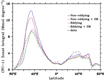
Fig. 2. Zonally integrated inventories of CFC-11 in 1994 as ob-served (black dashes, GLODAP) and as simulated by the noneddy-ing model with GM (red) and without GM (blue) as well as by the eddying model with GM (green) and without GM (purple).
personal communication). Our approach accounts for the an-thropogenic perturbation in CO2atmospheric concentrations
unlike Toggweiler et al. (1989b) who used the pre-industrial level for the atmospheric forcing. We force the 3-box atmo-sphere to maintain observed values of bomb 114C that were shifted upward by subtracting off values from July 1954, which are negative due to the Suess effect. Bomb 114C en-ters the ocean via air-sea exchange of CO2. Radioactive
de-cay is included but not important for the short simulations made here.
Following Orr et al. (2001), the air-sea bomb 114C flux
F14Ccan be expressed as:
F14C=µ(Ca−Co)(1 − I ) (5)
where Ca is atmospheric bomb 114C ratio, Cois the
simu-lated surface ocean ratio, and the CO2replenishment rate µ
is given by
µ = KCO2
pCO2a
DIC (6)
where DIC is the surface ocean concentration of dissolved inorganic carbon (taken as 2.0 mol m−3) (Toggweiler et al., 1989a).
3 Results
3.1 Model evaluation
3.1.1 GM parameterisation
Simulations with and without the GM parameterisation re-veal the extent to which the noneddying model with the GM
Fig. 3. Zonally integrated basin-scale inventories of CFC-11 for the Atlantic (upper), Pacific (middle), and Indian (lower) Oceans as observed (black dashes, GLODAP) and as simulated by the eddying (red) and noneddying (blue) models at end of year 1994.
parameterisation properly represents how CFC-11 is affected by mesoscale eddies in the eddying model. Figure 2 com-pares simulations of the eddying and noneddying models, both with and without GM, to the GLODAP global data product (Key et al., 2004) in terms of the vertical column integral of the CFC-11 concentration (inventory), integrated zonally across the globe. The eddying model matches the observed maximum in the CFC-11 inventory between 45◦S and 50◦S within 6%, whether or not it uses GM. In con-trast, the noneddying model without GM overestimates this peak by 55%. Although the noneddying model with GM is better, it still overestimates the observed peak by 36% and remains far from the eddying model. This unrealistic re-sult may be related to GM being an adiabatic parameteri-sation. There is an important diabatic component to eddy fluxes close to boundaries, particularly near the ocean surface (Robbins et al., 2000; Price, 2001). Thus GM misrepresents eddy diapycnal behaviour in the mixed layer and that may drive spurious exchange between the upper mixed layer and the ocean interior. But whatever the cause, our simple global analysis demonstrates that the GM parameterization in the noneddying model does not properly represent the role of mesoscale eddies in the eddying model. From here on then, we focus on the effect of resolution by comparing eddying and noneddying simulations without the GM parameterisa-tion.
3.1.2 CFC-11
The global CFC-11 inventory in the noneddying model is 28% larger than that obtained by the eddying model, with the latter being closer to the observed estimates (Key et al., 2004; Willey et al., 2004) (see Table 3). Both gridded data products rely on the WOCE CFC-11 observations although they use different interpolation procedures. In addition, the global inventory of our eddying model is close to that of the global 1/10◦eddy-resolving model of Sasai et al. (2004). As for meridional structure, Fig. 3 compares CFC-11 inven-tories from both models to the GLODAP data-based prod-uct (Key et al., 2004) over each of the three ocean basins. Higher resolution offers substantial improvement, particu-larly in the Indian basin where the coarse-resolution model overestimates the CFC-11 inventory by 64% between 50◦S and 30◦S. Conversely, south of 50◦S near the Antarctic di-vergence, both model versions underestimate the observed inventory, mainly because the mixed layer is too shallow by 150 to 200 m (Fig. 4). This model deficiency in the upper ocean of the high southern latitudes is associated with insuffi-cient vertical mixing produced by the current version of TKE scheme in OPA model. Additionally, formation of Antarctic Bottom Water (AABW) may be too weak. Yet despite this poor performance in the highest southern latitudes, there is little impact on basin-integrated inventories because discrep-ancies occur in a region that has relatively little surface area and tracer storage.
Fig. 4. Mixed-layer depth (m) in the southern extratropics in mid-September as simulated by the non-eddying (top) and eddying (middle) models as well as that from an observational climatology (de Boyer Mont´egut et al.,
2004) (bottom). 31
Fig. 4. Mixed-layer depth (m) in the southern extratropics in mid-September as simulated by the noneddying (top) and eddying (middle) models as well as that from an observational climatology (de Boyer Mont´egut et al., 2004) (bottom).
Simulated CFC-11 column inventories were also com-pared to observations along three sections in the southern extratropics: AJAX along the Greenwich meridian in 1983 (Warner and Weiss, 1992), WOCE I9S along 115◦E in the Indian Ocean (1994–1995), and WOCE P15 along 170◦W in the South Pacific in 1996 (Fig. 5). Once again, increased
0 1 2 3 4 5 6 7 8 64°S 60°S 56°S 52°S 48°S 44°S 40°S C F C -1 1 i n v e n to ry ( x 1 0 -6 m o l/ m 2 ) non-eddying eddying data 0 1 2 3 4 5 6 7 8 70°S 60°S 50°S 40°S 30°S 20°S 10°S Eq C F C -1 1 I n v e n to ry ( x 1 0 -6 m o l/ m 2 ) non-eddying eddying data Sasai 2004 0 1 2 3 4 5 6 7 8 68°S 60°S 52°S 44°S 36°S 28°S 20°S C F C -1 1 i n v e n to ry ( x 1 0 -6 m o l/ m 2 ) non-eddying eddying data Sasai 2004
Fig. 5. CFC-11 inventories for the WOCE I9S section along 115◦E in the Indian sector of the Southern Ocean (upper), the AJAX sec-tion along 0◦E in the South Atlantic (middle), and the WOCE P15S section along 170◦W in the South Pacific (lower), as observed (black) and as simulated by the noneddying (blue) and the eddy-ing (red) models. The dashed purple curves show the Sasai et al. (2004) inventories.
resolution improves results north of 50◦S in all three sec-tions. The noneddying model overestimates observed CFC-11 inventories along all three sections, as do most of OCMIP
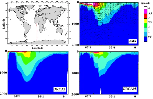
Fig. 6. CFC-11 concentration (in pmol l−1) along the WOCE I9S section (115◦E, 1994–1995) as observed and simulated by the noneddying (ORCA2) and the eddying (ORCA05) model.
coarse-resolution models that do not account for mesoscale processes (Dutay et al., 2002).
For greater detail south of 40◦S, where the ocean storage is largest and where OCMIP models differ most (Dutay et al., 2002), we compared models to data along two deep sections: I9S in the Indian sector of the southern extratropics (Fig. 6) and AJAX in the South Atlantic (Fig. 7). As seen with Fig. 5, finer resolution leads to general improvement, particularly along the Indian section. Most notable is the eddying model’s more realistic vertical penetration of CFC-11 north of Sub-antarctic Front (SAF), near 50◦S. In the noneddying simula-tion, the vertical distribution is too diffusive which results in excessive penetration particularly in the Indian Ocean. South of 50◦S, both model versions underestimate tracer
penetra-tion within the upper 200 m. We also compared modelled and observed CFC-11 in the North Atlantic on the Na20w merid-ional section, which runs mostly along 20◦W (Fig. 8). Both the eddying and noneddying models reproduce the general features of the CFC-11 vertical penetration profile, but in the noneddying model, there appears to be too much ventilation where NADW forms between 55◦N and 60◦N. Overall, the eddying model is also more realistic along this North Atlantic meridional section.
3.1.3 Anthropogenic CO2and bomb 114C
Unlike for CFC-11, both the noneddying and eddying mod-els simulate global anthropogenic CO2 inventories that are
within the uncertainty of GLODAP data-based estimate (Key et al., 2004; Sabine et al., 2004) (Table 3). For the global bomb 114C inventory, there is much less disagreement be-tween models, and again both agree within the uncertainty of the data-based estimate. The meridional structure of the bomb 114C inventory also differs very little between the models and the data-based estimate (Fig. 9). On the other hand, the meridional structure of anthropogenic CO2
inven-tory differs much more between models and the data-based estimate (Fig. 10). In the southern extratropics, the eddying model’s inventory is 26% less than that in the noneddying model, which is greater in magnitude than the 18% reduc-tion in global inventory. As for CFC-11, the eddying model also generally captures the magnitude and pattern of the data-based estimates for anthropogenic DIC, despite some dis-agreement in the tropical and subtropical Pacific Ocean as well as south of the SAF. In those high southern latitudes, the eddying model underestimates the data-based estimates for anthropogenic DIC (Key et al., 2004; Sabine et al., 2004),
Fig. 7. CFC-11 concentration (in pmol l−1) along the AJAX section (0◦E, 1983) as observed and simulated by the noneddying (ORCA2) and the eddying (ORCA05) model.
Fig. 8. CFC-11 concentration (in pmol l−1) along the Na20w section (1993) as observed and simulated by the noneddying (ORCA2) and the eddying (ORCA05) models
Fig. 9. Global zonal integral of the bomb 114C inventory as ob-served (black dashes, GLODAP) and as simulated by the noneddy-ing (blue) and eddynoneddy-ing (red) models at end of year 1994.
partly because the mixed-layer depth is too shallow (Fig. 4) as discussed already for the same deficiency that was re-vealed by CFC-11.
Unfortunately, systematic errors in the data-based esti-mates for anthropogenic DIC (Matsumoto and Gruber, 2005) compromise our ability to use that tracer by itself as a refer-ence to validate models (Orr et al., 2001). Anthropogenic DIC is clearly not of the same value as CFC-11, which is measured directly. Yet, trends for anthropogenic DIC are similar to those for CFC-11, i.e., in terms of the system-atic differences between the models and the data reference. This would be expected if the data-based estimates for an-thropogenic DIC were roughly correct. In any case, through-out the sthrough-outhern extratropics there are striking differences be-tween the noneddying and eddying models for both CFC-11 and anthropogenic DIC; for both tracers, the eddying model is much closer to the data reference. Having studied how each tracer is affected by improved resolution, we now turn our attention to how the three tracers differ in terms of ocean uptake, inventory, and northward transport.
3.2 Tracer-tracer differences
3.2.1 Ocean uptake
Figure 11a shows the zonal integrals of the cumulative fluxes for the three tracers obtained using the noneddying model. Cumulative fluxes are calculated as the time-integrated air-to-sea fluxes since the beginning of the simulations, and for comparison they are normalised by dividing by the total global uptake. Although all three tracers exhibit maximum uptake between 40◦S and 50◦S, the relative amount that is taken up south of 20◦S varies: 65% for CFC-11, 56% for anthropogenic CO2, and 50% for bomb 114C. These
dissim-Fig. 10. Inventories of anthropogenic CO2at the end of 1994
inte-grated zonally over each of the Atlantic (top), Pacific (middle), and Indian (bottom) basins for the data-based estimates (black dashes, GLODAP) as well as the noneddying (blue) and eddying (red) mod-els.
Fig. 11. Zonal integral of the normalised cumulative fluxes (upper)
and inventories (lower) of CFC-11 (red), anthropogenic CO2, (blue)
and bomb 114C (purple) in the noneddying model at end of 1994. Cumulative fluxes and inventories were normalised by dividing by the total global uptake.
ilarities are due to the differences between the three tracers in terms of their air-sea equilibration times and atmospheric histories (i.e., different shapes and rates of change). When combined with local differences in stratification and surface-layer residence times, these lead to different tracer uptake patterns. Figure 12 presents the corresponding cumulative flux maps for the three tracers normalised by dividing each by its area-weighted average surface flux.
Clearly oceanic uptake is not distributed evenly over the different basins. For example, the Atlantic Ocean absorbs up to 39% of the total CFC-11 uptake, although it covers only 26% of the total ocean area. For the two anthropogenic carbon tracers, there are smaller contrasts in uptake between basins, with the relative contribution of the Atlantic Ocean shrinking to 30% for anthropogenic CO2and 27% for bomb
114C.
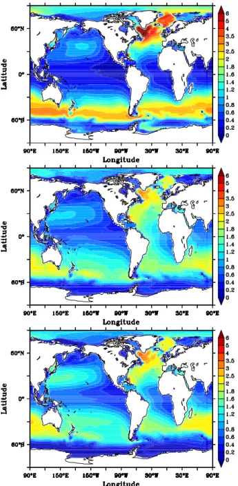
Fig. 12. Normalised cumulative fluxes simulated by the
noneddy-ing model for CFC-11 (upper), anthropogenic CO2(middle), and bomb 114C (lower), accumulated since the beginning of each sim-ulation until the end of year 1994. Fluxes were normalised by di-viding each field by the global area-weighted mean flux; thus there are no units.
The air-sea fluxes of the three tracers also differ in their responses to increasing horizontal resolution (Fig. 13). The bomb 114C uptake is nearly unchanged, both regionally and globally. In contrast, CFC-11 and anthropogenic CO2air-sea
fluxes decrease by 28% and 25% in the southern extratrop-ics and by 22% and 18% in the World Ocean. The reduction
Table 1. Changes in integrated global- and basin-scale, air-to-sea tracer fluxes when moving from the noneddying to the eddying model. CFC-11 CO2 114C Atlantic –34% –21% –4% Pacific –10% –12% –4% Indian –23% –24% –6% South of 20◦S –28% –25% –7% South of 50◦S –19% –23% –6% Global –22% –18% –5%
Table 2. Changes in integrated basin-scale tracer inventories when
moving from the noneddying to the eddying model. CFC-11 CO2 114C Atlantic –23% –18% –6% Pacific –11% –14% –2% Indian –37% –25% –7% South of 20◦S –31% –26% –9% South of 50◦S –44% –35% –14% Global –22% –18% –5%
of the air-sea CFC-11 flux is largest in the Atlantic Ocean (34%), moderate in the Indian (23%), and weakest in the Pa-cific (∼10%). Discrepancies between basins are less impor-tant for the air-sea flux of anthropogenic CO2(Table 1). In
both model versions, the peak uptake for CFC-11 remains south of 58◦S and that for bomb 114C remains at 52◦S; conversely, the peak uptake for anthropogenic CO2 shifts
from 57◦S to 54◦S with the increase in horizontal resolu-tion (Fig. 13). Later we show that this shift in the peak for anthropogenic CO2also affects its northward transport.
3.2.2 Inventories
Figure 11b shows each tracer’s normalised zonal integral inventory in the coarse-resolution model. More than 62% of the global inventory of CFC-11 is stored south of 20◦S, whereas only 49% of total uptake of anthropogenic CO2and
47% of bomb 114C are stored in this same region. That is, the relative contribution of the southern extratropical to the total air-sea flux is larger for CFC-11 than for the two other tracers (Fig. 11a).
Maps of these quantities (Fig. 14) reveal that the highest specific inventories (i.e., mass per unit area) for CFC-11 are found in the North Atlantic and between 30◦S and 50◦S. For the other tracers, the Atlantic Ocean also exhibits the highest specific inventories, but the contrast between basins is less for anthropogenic CO2 and less still for bomb 114C. As
for the vertical distributions, nearly 80% of the total
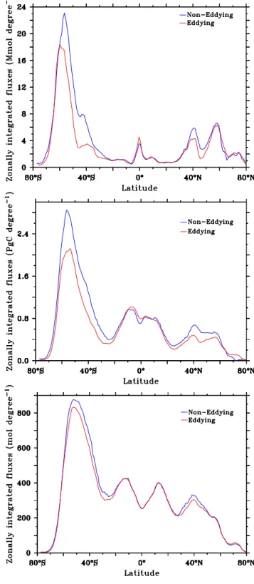
anthro-Fig. 13. Zonal integrated cumulative fluxes at the end of 1994 for CFC-11 (upper), anthropogenic CO2 (middle), and bomb
114C(lower) simulated by the noneddying (blue) and eddying mod-els (red).
Fig. 14. Normalised inventories simulated in the noneddying model
obtained by dividing by the mean area-weighted inventory for CFC-11 (top), anthropogenic CO2(middle), and bomb 114C (bottom) at end of year 1994.
pogenic CO2and around 90% of CFC-11 and bomb 114C
that is taken up by the ocean is stored in the upper 1000 m. Thus the large majority of the total inventory of these tran-sient tracers are confined above the thermocline. The only place where large tracer concentrations penetrate to mid and abyssal depths is in the North Atlantic as a result of the for-mation of the North Atlantic Deep Water (NADW). These findings are consistent with previous observational studies (Sabine et al., 2004; Willey et al., 2004). Thus our
analy-Table 3. Global inventories of the three transient tracers from the
data-based estimates (Key et al., 2004; Willey et al., 2004; Sabine et al., 2004) and as simulated by ORCA2, ORCA05, and the eddy resolving model from Sasai et al. (2004).
CFC-11 CO2 114C (106mol) (Pg C) (1028atoms14C) ORCA2 (noneddying) 648 120 3.07 ORCA05 (eddying) 506 98 2.94 GLODAP 544 (±81) 106 (±16) 3.13 (±0.47) Willey et al. (2004) 550 – – Sasai et al. (2004) 510 – – Sabine et al. (2004) – 106 –
sis remains focused on the upper and intermediate ocean. The decrease in air-sea fluxes of CFC-11 and anthro-pogenic CO2that accompanies increased horizontal
resolu-tion leads to equivalent reducresolu-tions in the global tracer inven-tories of these two tracers. Yet, this global decrease does not occur homogeneously throughout the three basins (Table 2). With increased resolution, both tracers show nearly the same decreases in uptake and storage in the Pacific Ocean. In con-trast, the reduction in storage is more pronounced in the In-dian Ocean and less pronounced in the Atlantic Ocean rela-tive to the reduction in uptake. Thus higher model resolution leads to greater lateral export of CFC-11 and anthropogenic CO2from the Indian to the Atlantic Ocean. It is well known
that heat and mass are exchanged between these two basins mainly via the Agulhas Current and the Antarctic Circum-polar Current (ACC), each of which is characterised by high eddy activity (Gordon, 1986; Rintoul, 1991). We hypoth-esise that the eddying model’s lower Indian-to-Atlantic net export of CFC-11 and anthropogenic CO2result from some
combination of stronger Agulhas transport and weaker ACC transport. Both effects are known to be induced by eddies (Hallberg and Gnanadesikan, 2001). Thus, eddies play a role in the inter-basin transport of transient tracers. One might also expect that eddies contribute to meridional transport of transient tracers.
3.2.3 Northward transport
To detail meridional or northward transport of a transient tracer, we first computed tracer divergence as the zonal in-tegral of the difference between cumulative flux and column inventory. Positive divergence (Flux – Inventory) indicates areas of tracer export or loss; negative divergence indicates areas of tracer gain. Both are due to meridional transport. The integral of the tracer divergence from south to north is the time-integrated northward transport since the beginning of simulation (Fig. 15).
For bomb 114C, the meridional distribution of the north-ward transport is nearly the same for the two versions of
the model. Yet for CFC-11, there is a decrease of equator-ward transport in the Northern Hemisphere between 0◦N and
45◦N, which is largest at 35◦N. In contrast, in the
south-ern extratropics, meridional transport of CFC-11 changes lit-tle with improved horizontal resolution. For anthropogenic CO2, the decreased equatorward transport due to increased
horizontal resolution is a general feature that occurs in both the Southern and the Northern Hemispheres, between 60◦S and 50◦N. These discrepancies between tracers result from their contrasting vertical distributions in the upper ocean. For example, the horizontal gradients of anthropogenic CO2and
of CFC-11 are of opposite signs within the thermocline (see Sect. 4.3). Gaining more insight into the exact mechanisms that drive these contrasts requires further study, which we leave for future work.
4 Discussion
For insight into how mesoscale eddies affect transient tracer distributions, we explored the main differences between the dynamics of the eddying and the noneddying simulations.
4.1 Eddies and stratification
In the higher southern latitudes, the simulated mixed layer is generally shallower in the eddying model (Fig. 4). The largest differences are found in the Indian and Atlantic basins between 40◦S and 60◦S, where the winter mixed layer in the eddying model is locally 200 to 300 m shallower than in the noneddying model. Relative to the observations be-tween 40◦S and 50◦S (de Boyer Mont´egut et al., 2004),
the simulated mixed layers are too deep in both models, particularly for the noneddying model in the Indian Ocean (de Boyer Mont´egut et al., 2004). The eddying model’s in-creased horizontal resolution substantially reduces the spu-rious wintertime convection in the higher southern latitudes. This reduction, due to explicitly including mesoscale eddies, is consistent with previous findings for the effect of Gent & McWilliams eddy parameterisation (Gent and McWilliams, 1990; Gent et al., 1995) on the strength of wintertime con-vection in the high southern latitudes (Hirst and McDougall, 1996; England and Hirst, 1997). Because convection is tied to water column stratification, we may anticipate that there are major changes in stratification between the two experi-ments. Indeed, increased resolution changes simulated sub-surface density between 60◦S and 40◦S by flattening
isopy-cnal surfaces. That flattening strengthens upper ocean strati-fication and yields a more realistic vertical density structure in the high southern latitudes. More specifically, baroclinic mesoscale eddies serve to release Available Potential Energy (APE) of the mean flow in the form of Eddy Kinetic Energy (EKE), thereby reducing the baroclinic instability and ensur-ing a more stable stratification. Marshall et al. (2002) also showed with idealised numerical experiments that mesoscale
Fig. 15. Total northward transport of CFC-11 (top), anthropogenic
CO2(middle), and bomb 114C (bottom) since the beginning of each simulation until 1994 as simulated by the noneddying (blue) and the eddying (red) models at end of year 1994.
Fig. 16. Zonal mean of CFC-11 penetration depth [m] as ob-served (black dashes, GLODAP) and as simulated by the noneddy-ing (blue) an eddynoneddy-ing (red) models over the Southern Hemisphere. The penetration depth of a tracer is defined as the tracer inventory [mol m−2] divided by its surface concentration [mol m−3].
eddies play a key role in setting up the stratification. By strengthening vertical stratification in the high southern lati-tudes, mesoscale eddies affect the rate at which the thermo-cline and intermediate waters are ventilated as well as how water masses are transformed within the upper ocean. As a consequence of the flattening of density surfaces, vertical penetration of CFC-11 and anthropogenic CO2are reduced
in the eddying model (Fig. 16).
4.2 Ventilation and upper water mass transformation
Higher resolution and thus the presence of mesoscale ed-dies reduces the excessive vertical penetration of simulated CFC-11 between 60◦S and 40◦S (Fig. 6). For example, be-tween 55◦S and 50◦S, waters at 1000 m contain more than 2 pmol l−1 of CFC-11 in the noneddying model but only around 0.5 pmol l−1in the eddying model (as in the obser-vations). Most of the CFC-11 that penetrates into subsurface waters south of 40◦S is carried by Subantarctic Mode Wa-ter (SAMW) and Antarctic InWa-termediate WaWa-ter (AAIW) as they subduct near the SAF. In the SAMW layer (σ0=26.5
to 27.0), the CFC-11 inventory between 60◦S and 40◦S is nearly twice that in the AAIW layer (σ0=27.0 to 27.4). Yet
that SAMW inventory is only 2% less in the eddying model relative to the noneddying model, whereas the corresponding inventory reduction in the AAIW is 20%. Thus we focus on the AAIW. That intermediate water is easily identified as a tongue of fresh water with a salinity minimum of 34.2 and a mean potential density of ∼27.2. The AAIW extends north-ward from the Antarctic Polar Frontal Zone (APFZ), which is located near the Antarctic Divergence along the southern flank of ACC, to intermediate depths at subtropical latitudes. The AAIW’s CFC-11 inventory (Fig. 17) illustrates that the
Fig. 17. Zonal integral of CFC-11 inventory (106mol) in the AAIW, defined as the 27.0–27.4 σ0layer as observed (black dashes, GLO-DAP) and as simulated by the noneddying (blue) and the eddying (red) models.
noneddying model’s excessive ventilation of that water mass is responsible for much of the excessive vertical penetration of transient tracers in the southern extratropics. The noned-dying model overestimates the AAIW’s observed CFC-11 content in all basins, particularly in the Atlantic and in the In-dian sectors of the Southern Ocean, where the excess reaches more than a factor of two. The 20% reduction in the AAIW’s CFC-11 inventory between 60◦S and 40◦S is accompanied by decreases in the total volume of the AAIW layer, by 33% between 60◦S and 50◦S and by 19% between 50◦S and 40◦S. Thus, the strong ventilation of the upper and the inter-mediate ocean in the southern extratropics in the noneddying model is partly linked to its excessive AAIW formation rate. To better understand the source of AAIW, the merid-ional circulation, and the water mass transformations that oc-cur in upper waters (above the permanent thermocline) be-tween 40◦S and 65◦S, we calculated the isopycnal trans-port streamfunction in both the eddying and noneddying versions of the model. Averaging along density instead of depth coordinates avoids the spurious large apparent di-apycnal motion in the upper Southern Ocean known as the Deacon Cell (D¨o¨os and Webb, 1994). When the isopycnal streamfunction is given on neutral density surfaces, McIn-tosh and McDougall (1996) showed that it approximates the so-called residual mean circulation, which is the sum (calcu-lated in depth coordinates) of the Eulerian circulation and the eddy-induced flow (Andrews and McIntyre, 1976; Holton, 1981). Near the ocean surface, where eddies are most ac-tive, neutral surfaces are tangential to σ0 potential density
surfaces (McDougall, 1987). Following the lead of (D¨o¨os and Webb, 1994), we computed the isopycnal
streamfunc-Fig. 18. The isopycnal transport streamfunction (in Sv) plot-ted in σ0 coordinate for the noneddying (ORCA2) and eddying
(ORCA05) models for the region south of 40◦S. The contour in-terval is 5 Sv. The purple line indicates the position of the annual maximum mixed layer depth in density space. Positive values indi-cate clockwise circulation.
tion relative to the surface (σ0) by projecting model output
onto 72 evenly spaced potential density layers ranging from 21 to 28 (Fig. 18). Yet, due to compressibility effects, deeper water masses, including the Lower Circumpolar Deep Wa-ter (LCDW), NADW, and AABW, are not well defined by
σ0. Thus a σ0-based separation between NADW and LCDW
would be misleading. Here we consider these denser water masses as a unique layer (27.6–28.1 density class).
In the noneddying simulation, the residual circulation in the upper ocean south of 40◦S is characterised by a small Deacon Cell with a maximum of 30 Sv at 58◦S near the Antarctic Divergence. Although unrealistic, such large meridional circulation is not surprising given that this model has no eddies, which in the real ocean counter part of the Ekman driven transport. In an observational study, Karsten and Marshall (2002) found a northward Ekman driven trans-port of more than 23 Sv between 51◦S and 57◦S. The
equiv-alent northward transport in our noneddying model is as-sociated with excessive upwelling of about 26 Sv of dense water (27.6–28.1) that is transported across the 27.5 sur-face between 65◦S and 58◦S. Most of this water that feeds the AAIW formation lies within the “bowl”, which sepa-rates the subsurface ocean from the interior ocean (Marshall and Nurser, 1992), thereby directly ventilating the upwelled dense waters. Therefore, the excessive upwelling rate is closely linked to the overestimation of AAIW ventilation in the noneddying version of the model.
Fig. 19. Four-year trajectories of 10 particles launched from 250 m
at 60◦S, between 110◦E and 120◦E. Colours represent the depth of the particles.
In the eddying simulation, due to the countering effect of eddy-induced transport, the Deacon Cell nearly disappears and the residual circulation is roughly halved to 14 Sv of northward near-surface transport between 55◦S and 60◦S. Consequently, the upwelling of the dense water masses along the southern flank of the ACC is substantially reduced. In the eddying model only 12 Sv is upwelled across the 27.5 σ0
surface between 65◦S and 58◦S. This model result is con-sistent with the observational study of Karsten and Marshall (2002) who found a residual circulation of about 13 Sv at 57◦S. The large reduction in upwelling of denser, tracer-impoverished waters results in an equally large decrease in AAIW ventilation (Fig. 17). Additionally, Fig. 18 reveals that the diapycnal flux diminishes with increased resolution as the isopycnal overturning streamlines become flatter. This makes sense given that eddies facilitate meridional circula-tion along isopycnal surfaces (Hallberg and Gnanadesikan, 2001). These eddy-induced reductions in water mass trans-formation within the upper waters of high southern latitudes lead to reduced air-sea fluxes of transient tracers, as detailed below.
4.3 Surface water saturation and residence time
Within the surface and intermediate waters of the southern high latitudes, eddies act to weaken the residual circula-tion, which is northward at the surface. To illustrate this eddy-induced slowdown of the residual circulation south of 40◦S, we examined the Lagrangian trajectories of individ-ual particles that were launched from under the mixed layer of the upwelling region south of the ACC. For this analy-sis, we relied on the Lagrangian diagnostic tool ARIANE (Blanke and Raynaud (1997), which is fully documented at http://fraise.univ-brest.fr/∼blanke/ariane/doc.html).
Fig-ure 19 shows 4-year trajectories of particles launched from just below the mixed layer in the Indian Ocean at 60◦S between 140◦E and 120◦E. In the noneddying model,
wa-ter parcels upwell to the surface and are rapidly transported northward across the ACC, whereas in the eddying model they spend more time in the mixed layer before they are transported northward. Thus with higher resolution, there is an increase in the residence time of water parcels at the surface in the southern high latitudes where air-sea tracer fluxes are largest. Consequently, tracers have more time to accumulate in surface waters between 60◦S and 40◦S. For tracers whose equilibration times are relatively short (CFC-11 and anthropogenic CO2), surface water concentrations
in-crease and become closer to equilibrium with the atmosphere (Fig. 20). For example, at 53◦S the magnitude of the air-sea difference in the partial pressure of CFC-11 in the eddying model is only half that in the noneddying model. This re-duction along with the reduced upwelling of tracer impover-ished waters from below explains why the increased resolu-tion reduces cumulative air-sea fluxes of CFC-11 and anthro-pogenic CO2.
On the other hand, 14C’s slow air-sea equilibration time of ∼6 years is too long, relative to the increase in residence time of surface waters, to allow surface-water levels of bomb
114C to become as close, relatively speaking, to the atmo-spheric level. For example, the average level of bomb 114C in the atmosphere over the southern extratropics was at 144 permil in 1994. Refining resolution increased surface-ocean bomb 114C from 61 to 69 permil at 53◦S (Fig. 21). This represents only a 10% reduction in the air-sea difference for bomb 114C (i.e., Ca−Co in Eq. (5)), which is much less
than the 50% reduction for the air-sea difference in the par-tial pressure of CFC-11 mentioned above. The small relative decrease in the air-sea difference for bomb 114C at 53◦S is
comparable in magnitude to the corresponding reduction in the bomb 114C flux in the same area (Table 1), i.e., near where fluxes are largest. Despite its differences, bomb 114C is carried by the same circulation and is submitted to the same vertical mixing as the two other anthropogenic tracers. Eddy-induced changes in vertical mixing within the ocean interior affect the vertical distributions of all three tracers. Below the thermocline, concentrations of all three tracers de-crease (Fig. 21) because as the resolution is refined, the water
Fig. 20. Zonal mean of the CFC-11 saturation index in the At-lantic between 60◦S and 40◦S for the noneddying (blue) and ed-dying (red) models. The CFC-11 saturation index is defined as:
SI =100×(pop−pa
a ), where poand paare CFC-11 partial pressures
at ocean surface and in the atmosphere respectively.
column becomes more stratified. Thus, enhancing resolution decreased vertical penetration of all three tracers (Fig. 21).
In the previous analysis, we highlighted the role of con-trasting equilibration times between the three tracers to ex-plain why the bomb 114C behaves so differently from the two other tracers. Additionally, the three tracers differ in terms of the shape of their atmospheric history (Fig. 22). To discriminate between these two factors, we made another type of14C simulation, where instead of the nuclear-era per-turbation, we accounted for only the Suess effect, i.e., the reduction in the atmospheric14C/12C ratio due to the emis-sion of fossil CO2during the industrial era. This perturbation
simulation for the 114C Suess-effect was made in both mod-els over most of the industrial era, from 1839 to 1950, just prior to the beginning of the nuclear-era increase in atmo-spheric CO2. Although the air-sea equilibration time for this
114C Suess effect is identical to that for bomb 114C, the corresponding atmospheric histories are radically different. As opposed to the bomb pulse input, the Suess effect 114C exhibits a slow atmospheric decrease, similar in form to the anthropogenic CO2increase. In this way, we isolated the
ef-fect of the 114C time history. The magnitude of the Suess
114C perturbation that is absorbed by the global ocean is 8% less in the eddying model relative to that in the noned-dying model, whereas the corresponding difference is only 5% for bomb 114C in 1994. Although this 8% change for the C-14 Suess effect is larger than that for bomb 114C, it still remains less than 1/3 of that for anthropogenic CO2and
CFC-11. Therefore, the atmospheric history does matter, but the main reason why bomb 114C’s response to increasing resolution is so much weaker than for the other two tracers is due to its much longer air-sea equilibration time.
Fig. 21. Vertical profiles of zonally averaged concentrations of CFC-11 (upper), anthropogenic DIC (middle), and bomb 114C (lower) at 60◦S (left) and 40◦S (right) for the noneddying (blue) and eddying (red) models.
5 Summary and conclusions
The effect of mesoscale eddies on global distributions of CFC-11, anthropogenic CO2, and bomb 114C was
inves-tigated by comparing eddying and noneddying versions of the same coupled ocean-sea ice model ORCA-LIM. Our aim was to evaluate how explicitly simulating eddies affects three complementary anthropogenic tracers, particularly in the southern extratropics where ocean uptake, storage, and meridional transport of these tracers are largest.
Comparable simulations with noneddying and eddying versions of the same model showed that the improved resolu-tion led to reducresolu-tions in global ocean tracer uptake, by 22% for CFC-11 and by 18% for anthropogenic CO2. The largest
discrepancies occur in the Atlantic and Indian sectors of the southern extratropics. Conversely, eddies have little effect on global and regional bomb 114C uptake. By comparing basin-integrated cumulative fluxes and inventories, we found that eddies also affect inter-basin tracer exchange of CFC-11
-0.2 0 0.2 0.4 0.6 0.8 1 1765 1790 1815 1840 1865 1890 1915 1940 1965 1990 CFC-11 CO2 C14
Fig. 22. Atmospheric histories of CFC-11 (blue), anthropogenic CO2(black), and 114C (purple) over the prenuclear (prior to 1954)
and nuclear or “bomb” (after 1954) periods. For comparison, each of the three curves was normalised by dividing by its maximum tracer concentration; thus there are no units.
and anthropogenic CO2, substantially reducing
Atlantic-to-Indian Ocean tracer transport. Model-data comparison re-veals that moving from noneddying to eddying resolution substantially improved model performance, whereas using the GM parameterisation with the noneddying model offered only limited improvement.
Secondly, we sought to improve the general understand-ing of the role of eddies in the high southern latitudes. Our results indicate that taking the first step towards higher res-olution, moving from a coarse-resolution model to a model that begins to resolve mesoscale eddies, results in stronger upper ocean stratification in the high southern latitudes as manifested by a thinner mixed layer and flattened density surfaces. Eddies act to reduce AAIW-mediated ventilation of the intermediate waters, particularly in the Indian sector of the southern extratropics. By diagnosing the upper merid-ional circulation of the southern extratropics within an isopy-cnal framework, we showed that enhancing resolution to ex-plicitly resolve mesoscale eddies decreases the AAIW for-mation rate in near-surface waters along the southern flank of ACC (at around 60◦S). This leads to weaker ventilation of the thermocline and intermediate ocean. Eddies act to reduce the upwelling of dense water near the Antarctic Divergence (60◦S–55◦S), leading to a similar reduction in near-surface
conversion of AAIW from 26 Sv in the noneddying model to 12 Sv in the eddying model at 58◦S, in close agreement with
the data-based estimate of Karsten and Marshall (2002). Because eddies reduce meridional circulation (residual cir-culation) in the upper waters of the southern extratropics, they also bring surface-water levels of CFC-11 and anthro-pogenic CO2closer to those in the atmosphere, thereby
re-ducing air-sea tracer fluxes. Refining resolution to explic-itly simulate eddies increases surface residence time between
60◦S and 50◦S, where air-sea tracer fluxes are the largest, as
illustrated by our Lagrangian trajectory analysis of particles launched from just below the mixed layer at 60◦S in the
up-welling zone of the Indian sector of Southern Ocean. Unlike for CFC-11 and anthropogenic CO2, bomb 114C
air-sea fluxes are much less sensitive to the eddy-induced slowdown in upper meridional circulation. The long air-sea equilibration time of bomb 114C means it is slow to react during the relatively short period from when water masses are upwelled to the surface near the Antarctic Divergence until they are subducted a few degrees to the north near the SAF. Although the bomb 114C inventory is nearly identical in both the noneddying and eddying models, vertical pro-files of bomb 114C in these models differ. Refined resolu-tion increases concentraresolu-tions near the surface and decreases concentrations deeper down owing to the eddying model’s enhanced stratification and weaker ventilation of intermedi-ate wintermedi-aters. Bomb 114C’s much weaker sensitivity to in-creased resolution is mainly due to its slower air-sea equi-libration time, and not its pulse-shaped atmospheric history, as demonstrated by our sensitivity test for the preindustrial-to-prenuclear 114C perturbation (Suess effect).
Despite similarities between these three anthropogenic tracers, their contrasting sensitivities to the mesoscale eddies reemphasise that we must be careful when trying to use find-ings from CFC-11 and bomb 114C to make inferences about
anthropogenic CO2. We do not know if ocean model
esti-mates of anthropogenic CO2would be altered substantially
by further increases in horizontal resolution, but this study does emphasise the general need for ocean models to adopt higher resolution or improved subgrid-scale mixing parame-terisations. For instance in climate models, higher resolution should likewise lead to more realistic ventilation of interme-diate waters, which would alter decadal-scale ocean heat up-take.
Appendix A
Oceanic carbon perturbation δpCO2ocalculation
The equations used here are based on the perturbation ap-proach of Sarmiento et al. (1992). The oceanic perturba-tion δpCO2o is defined as the change in CO2 partial
pres-sure in the ocean from the beginning of the simulation (pre-industrial level). The plot of δpCO2o
δDIC versus δpCO2o, where
δDI Cis the concentration of dissolved inorganic carbon of the perturbation at the surface (in µmol kg−1), reveals a lin-ear relation for δpCO2o ranging from 0 to 200 ppm. Thus, we can express simply the oceanic carbon perturbation as a function of δDIC by
δpCO2o
where z0and z1are seasonally varying coefficients
depend-ing on temperature T (in degrees Celsius) as in Sarmiento et al. (1995)
z0=1.7561 − 0.031618 × T + 0.0004444 × T2 (A2)
z1=0.004096 − 7.7086 × 10⁻⁵×T +6.10 × 10⁻⁷×T2 (A3)
Rearranging Eq. (A1) and modifying to allow simulations to start at a different reference value than pCO2a,ref=280 ppm used in the original Siegenthaler and Joos (1992) equation for the perturbation approach gives
δpCO2o=
z0[δDIC + δDICcorr]
1 − z1[δDIC + δDICcorr]
−pCO2a,corr (A4) with δDICcorr= pCO2a,corr z0+z1×pCO2a,corr (A5) and
pCO2a,corr=pCO2a,0−pCO2a,ref=278 ppm − 280 ppm (A6)
Acknowledgements. We thank A.-M. Treguier, G. Madec, B. Barnier, and other DRAKKAR project members for discussions. We also thank S. Raynaud for his technical advice for using ARIANE and the ESOPA group at LOCEAN for the general support, improvements, and maintenance of the ocean model OPA-ORCA. Special thanks to GLODAP data providers. Support for this research has come from the French Commissariat `a l’Energie Atomique (CEA) and the EU CARBOOCEAN Project (Contract no. 511176 [GOCE]). Computations were performed at CEA (CCRT) supercomputing centre. The IAEA is grateful for the support provided to its Marine Environmental Laboratory by the Government of the Principality of Monaco.
Edited by: V. Garcon
References
Andrews, D. and McIntyre, M.: Planetary waves in horizontal and vertical shear: The generalized Eliassen-Palm relation and the mean zonal acceleration, J. Atmos. Sci., 33, 2031–2048, 1976. Arakawa, A.: Design of the UCLA general circulation model,
nu-merical simulation of weather and climate, Tech. Rep. 7, Univer-sity of California, Dept. of Meteorology, 1972.
Berliand, M. E. and Strokina, T.: Global distribution of the total amount of clouds (in Russian), Hydrometeorological Publishing House, Leningrad, Russia, 71 pp., 1980.
Blanke, B. and Delecluse, P.: Low frequency variability of the trop-ical Atlantic ocean simulated by a general circulation model with two different mixed layer physics, J. Phys. Oceanogr., 23, 1363– 1388, 1993.
Blanke, B. and Raynaud, S.: Kinematics of the Pacific Equatorial Undercurrent: an Eulerian and Lagrangian approach from GCM results, J. Phys. Oceanogr., 27, 1038–1053, 1997.
B¨oning, C. and Budich, R.: Eddy dynamics in a primitive equation model: Sensitivity to horizontal resolution and friction, J. Phys. Oceanogr., 22, 361–381, 1992.
Broecker, W. S. and Peng, T.-H.: Gas exchange rates between air and sea, Tellus, 26, 21–35, 1974.
Chassignet, E. P. and Verron, J.: Ocean Weather Forecasting: An Integrated View of Oceanography, Springer, 2006.
Chelton, D. B., deSzoeke, R. A., Schlax, M. G., Naggar, K. E., and Siwertz, N.: Geographical variability of the first-baroclinic Rossby radius of deformation, J. Phys. Oceanogr., 28, 433–460, 1998.
Cox, M.: An eddy resolving model of the ventilated thermocline, J. Phys. Oceanogr., 15, 1312–1324, 1985.
Crosnier, L., Barnier, B., and Tr´eguier, A.: Aliasing of inertial os-cillations in the 1/6◦Atlantic circulation Clipper model : impact on the mean meridional heat transport, Ocean Model., 3, 21–32, 2001.
de Boyer Mont´egut, C., Madec, G., Fischer, A. S., Lazar, A., and Iudicone, D.: Mixed layer depth over the global ocean: an exam-ination of profile data and a profile-based climatology, J. Geo-phys. Res., 109, C12003, doi:10.1029/2004JC002378, 2004. Doney, S. and Bullister, J.: A chlorofluorocarbon section in the
east-ern North Atlantic, Deep-Sea Res., 39, 1857–1883, 1992. D¨o¨os, K. and Webb, D. J.: The Deacon Cell and the other
merid-ional cells in the Southern Ocean, J. Phys. Oceanogr., 24, 429– 442, 1994.
Drijfhout, S.: Heat transport by mesoscale eddies in an ocean circu-lation model, J. Phys. Oceanogr., 24, 353–369, 1994.
Dutay, J.-C., Bullister, J., Doney, S. C., Orr, J. C., Najjar, R. G., Caldeira, K., Campin, J.-M., Drange, H., Follows, M., Gao, Y., Gruber, N., Hecht, M. W., Ishida, A., Joos, F., Lindsay, K., Madec, G., Maier-Reimer, E., Marshall, J. C., Matear, R., Mon-fray, P., Mouchet, A., Plattner, G. K., Sarmiento, J. L., Schlitzer, R., Slater, R. D., Totterdell, I. J., Weirig, M.-F., Yamanaka, Y., and Yool, A.: Evaluation of ocean model ventilation with CFC-11: Comparison of 13 global ocean models, Ocean Model., 4, 89–120, 2002.
England, M. H. and Hirst, A. C.: Chlorofluorocarbon uptake in a world ocean model 2. Sensitivity to surface thermohaline forcing and subsurface mixing parameterisation, J. Geophys. Res., 102, 15 709–15 731, 1997.
Enting, I., Wigley, T., and Heimann, M.: Future Emissions and Con-centrations of Carbon Dioxide: Key Ocean/Atmosphere/Land Analyses, Tech. rep., CSIRO Division of Atmospheric Research, 1994.
Fichefet, T. and Maqueda, M. M.: Sensitivity of a global sea ice model to the treatment of ice thermodynamics and dynamics, J. Geophys. Res., 102, 12 609–12 646, 1997.
Gaspar, P., Gregorius, Y., and Lefevre, J.-M.: A simple eddy kinetic energy model for simulations of oceanic vertical mixing tests at Station Papa and Long-Term Upper Ocean Study Site, J. Geo-phys. Res., 95, 16 179–16 193, 1990.
Gent, P. R. and McWilliams, J. C.: Isopycnal mixing in ocean cir-culation models, J. Phys. Oceanogr., 20, 150–155, 1990. Gent, P. R., Willebrand, J., McDougall, T. J., and McWilliams, J. C.:
Parameterising eddy-induced tracer transports in ocean circula-tion models, J. Phys. Oceanogr., 25, 463–474, 1995.
GLOBALVIEW-CO2: Cooperative Atmospheric Data Integration Project — Carbon Dioxide, CD-ROM, NOAA CMDL, Boulder,