HAL Id: hal-00329253
https://hal.archives-ouvertes.fr/hal-00329253
Submitted on 1 Jan 2003
HAL is a multi-disciplinary open access
archive for the deposit and dissemination of
sci-entific research documents, whether they are
pub-lished or not. The documents may come from
teaching and research institutions in France or
abroad, or from public or private research centers.
L’archive ouverte pluridisciplinaire HAL, est
destinée au dépôt et à la diffusion de documents
scientifiques de niveau recherche, publiés ou non,
émanant des établissements d’enseignement et de
recherche français ou étrangers, des laboratoires
publics ou privés.
cycles
S. E. Milan, M. Lester, S. W. H. Cowley, K. Oksavik, M. Brittnacher, R. A.
Greenwald, G. Sofko, J.-P. Villain
To cite this version:
S. E. Milan, M. Lester, S. W. H. Cowley, K. Oksavik, M. Brittnacher, et al.. Variations in the polar
cap area during two substorm cycles. Annales Geophysicae, European Geosciences Union, 2003, 21
(5), pp.1121-1140. �hal-00329253�
Annales
Geophysicae
Variations in the polar cap area during two substorm cycles
S. E. Milan1, M. Lester1, S. W. H. Cowley1, K. Oksavik2, M. Brittnacher3, R. A. Greenwald4, G. Sofko5, and J.-P. Villain6
1Department of Physics and Astronomy, University of Leicester, Leicester, UK 2Department of Physics, University of Bergen, Bergen, Norway
3University of Washington, Geophysics Program, Seattle, Washington, USA
4The Johns Hopkins University, Applied Physics Laboratory, Laurel, Maryland, USA
5Institute of Space and Atmospheric Studies, Department of Physics and Engineering, University of Saskatchewan,
Saskatchewan, Canada
6Centre National de la Recherche Scientifique, Orl´eans, France
Received: 6 September 2001 – Revised: 22 October 2002 – Accepted: 29 October 2002
Abstract. This study employs observations from several
sources to determine the location of the polar cap bound-ary, or open/closed field line boundbound-ary, at all local times, allowing the amount of open flux in the magnetosphere to be quantified. These data sources include global auroral im-ages from the Ultraviolet Imager (UVI) instrument on board the Polar spacecraft, SuperDARN HF radar measurements of the convection flow, and low altitude particle measurements from Defense Meteorological Satellite Program (DMSP) and National Oceanographic and Atmospheric Administration (NOAA) satellites, and the Fast Auroral SnapshoT (FAST) spacecraft. Changes in the open flux content of the mag-netosphere are related to the rate of magnetic reconnection occurring at the magnetopause and in the magnetotail, al-lowing us to estimate the day- and nightside reconnection voltages during two substorm cycles. Specifically, increases in the polar cap area are found to be consistent with open flux being created when the IMF is oriented southwards and low-latitude magnetopause reconnection is ongoing, and de-creases in area correspond to open flux being destroyed at substorm breakup. The polar cap area can continue to de-crease for 100 min following the onset of substorm breakup, continuing even after substorm-associated auroral features have died away. An estimate of the dayside reconnection voltage, determined from plasma drift measurements in the ionosphere, indicates that reconnection can take place at all local times along the dayside portion of the polar cap bound-ary, and hence presumably across the majority of the dayside magnetopause. The observation of ionospheric signatures of bursty reconnection over a wide extent of local times sup-ports this finding.
Key words. Ionosphere (plasma convection; polar
iono-sphere) – Magnetospheric physics (magnetospheric config-uration and dynamics)
Correspondence to: S. E. Milan ([email protected])
1 Introduction
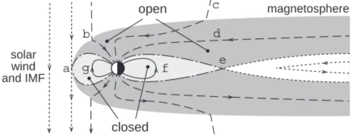
The ability to monitor the location of the polar cap bound-ary, the boundary between “closed terrestrial” magnetic flux and “open” flux interconnected with the solar wind, allows for the electrodynamics of solar-terrestrial coupling to be in-vestigated, specifically the storage and release of magnetic energy within the magnetosphere during the substorm cy-cle. We show the magnetosphere schematically in Fig. 1. In this diagram we make a distinction between interplanetary magnetic field (IMF) lines (dotted curves), closed terrestrial field lines (solid and dot-dashed curves), i.e. field lines con-nected to the Earth at both ends, and open field lines (dashed curves) which interconnect the Earth and the IMF. When the IMF has a southward component, reconnection takes place between the IMF and closed terrestrial field lines on the day-side magnetopause at point a (we will refer to this as “low-latitude reconnection”). This causes closed flux to become open, leading to an accumulation of open flux in the magne-tosphere, also resulting in an increase in the area of the polar cap, that region of the polar ionosphere that is threaded by open flux. An increase in polar cap size, produced by on-going low-latitude reconnection, is known as the substorm growth phase. As one end of open magnetic field lines are connected to the antisunward-flowing solar wind, they be-come swept into the magnetotail (b −d) where they represent stored magnetic energy. The closure of open magnetic flux through reconnection in the magnetotail (at point e) causes a decrease in the polar cap area, and occurs during the sub-storm expansion and recovery phases, representing a release of the stored magnetotail energy. Newly-closed field lines return to the dayside magnetosphere (f − g) where they can participate in reconnection at point a again. Down-tail of the nightside reconnection site (point e) field lines are once again unconnected with the Earth and return to the IMF. The cycle of magnetic field lines from closed to open to closed again, which results from day- and nightside reconnection, is known as magnetospheric convection or the Dungey
cy-magnetosphere open closed solar wind and IMF a b c d e f g
Fig. 1. A schematic diagram of the magnetosphere in the
noon-midnight meridian. The solar wind and IMF impinge from the left, IMF field lines represented by dotted curves. Full and dashed curves show closed and open field lines, respectively. The dot-dashed lines indicate the open/closed field line boundary, the ionospheric projec-tion of which is the polar cap boundary. Letters a to g indicate the evolution of field lines during the Dungey cycle.
cle. In Fig. 1, dot-dashed lines indicate the “last closed field lines” or the boundary between open and closed flux (the open/closed field line boundary or OCB), which maps to the polar cap boundary in the ionosphere. It is clear from this that for southward IMF, the reconnection sites a and e map to the polar cap boundary.
The reconnection processes at a and e are time-dependent phenomena, controlled by the IMF orientation upstream of the Earth on the dayside and by conditions in the magnetotail on the nightside. A knowledge, then, of variations in polar cap area permits quantification of these reconnection rates, that take place in regions which are difficult – if not impos-sible – to monitor in situ routinely. Reconnection also has ramifications for the ionosphere. The magnetospheric con-vection cycle leads to ionospheric plasma drift in the familiar twin-cell convection pattern, with antisunward flow across the polar cap (open field lines) and return flow at lower lati-tudes (closed field lines). This ionospheric convection, when combined with a knowledge of the location of the polar cap boundary, can also be used to quantify the rate of reconnec-tion.
In contrast to southward IMF conditions, when the IMF has a northward component “high-latitude reconnection” can take place with pre-existing open field lines in the magne-tospheric lobes (this might occur near b). Depending on whether individual solar wind magnetic field lines reconnect with both northern and southern lobes or reconnect with only one, it is thought that open magnetic flux can be closed or the amount of open flux in the system can remain unchanged, re-spectively (see Cowley, 1981, and references therein). In ei-ther case, a region of sunward ionospheric flow is predicted within the polar cap, and the dayside reconnection site no longer necessarily maps to the polar cap boundary. Again, measurements of changes in polar cap area should help un-derstand this phenomenon. For these reasons, this paper charts changes in polar cap area during two substorm cycles, to help elucidate the role of reconnection in the solar wind-magnetosphere-ionosphere system.
The relationship between the amount of open flux in the
system and the reconnection rate can be summarized by the following statement of Faraday’s Law (e.g. Siscoe and Huang, 1985; Lockwood and Cowley, 1992; Lewis et al., 1998):
BI
dApc
dt =8day−8night. (1)
Here, BIis the magnetic field strength in the ionosphere,
assumed to be constant over the polar region and approxi-mately equal to 5 × 10⁴nT, and Apc is the area of the polar
cap, that is the region penetrated by open field lines. Hence,
BIApcis the amount of open flux, Fpc, associated with each
hemisphere, necessarily equal in both. The RHS of Eq. (1) is the emf induced around the polar cap boundary (or, equally, the magnetic separatrix in the magnetosphere), which here we have resolved into two components, the day- and night-side reconnection voltages 8day and 8night. The
reconnec-tion voltages are the integrals of the day- and nightside recon-nection electric fields along those portions of the polar cap boundary, or open/closed field line boundary (OCB), which map to the reconnection sites or “merging gaps”. These re-connection electric fields, Er, are associated with E × B
plasma drift in the ionosphere, perpendicular to the bound-ary, and so the change in area of the polar cap should also be related to the convection flow across the boundary in unit time. The reconnection electric field is measured in the frame of reference of the boundary, and so motions of the bound-ary itself, for instance, moving equatorward as the polar cap expands during substorm growth phase, must be taken into account.
Lockwood et al. (1990), Cowley and Lockwood (1992), Cowley et al. (1992) and Lockwood and Cowley (1992) give a framework within which changes in the amount of open flux in the polar cap can be understood. Initially, it is as-sumed that the open and closed flux of the magnetosphere are in a state of equilibrium and that the polar cap is cir-cular, containing flux Fpc. In response to a pulse of
day-side reconnection, a region of closed flux 1Fpc adjacent to
the pre-existing dayside polar cap boundary is opened in the time interval 1t . By definition, the OCB – the boundary which encloses open flux – has then moved equatorwards to encompass this new open flux. If the merging gap is of length
land reconnection is uniform along it, then the OCB moves equatorwards by a distance 1F /BIl everywhere along that
length, to enclose the new flux, and the velocity of the bound-ary motion is 1F /BIl1t. Although in the present
exam-ple the plasma flow in the frame of reference of the Earth is zero, in the frame of the boundary there is an E × B drift of magnitude v0 =Er/BI, driven by the reconnection
elec-tric field Er, and hence, Er = 1F / l1t. The reconnection
voltage, the integral of Er along the merging gap, is seen
to be 8day = 1F /1t, equivalent to Eq. (1). The OCB is
now distended on the dayside, having departed from its equi-librium shape. Plasma flows are excited in the Earth’s ref-erence frame to return the system to equilibrium (a circular polar cap) once again, that is a poleward motion in the region of new open flux and an equatorward motion at other local
times around the OCB. At this stage there is no plasma flow across the OCB, that is the OCB moves with the plasma flow – it is said to be “adiaroic”, meaning “no flow across” (Sis-coe and Huang, 1985) – and the electric field in the frame of the boundary is zero. To achieve this redistribution of the flux and to return the OCB to its circular equilibrium state, these plasma flows will have the familiar twin-cell pattern of the convection flow (e.g. Heppner and Maynard, 1987; Ruohoniemi and Greenwald, 1996). The new location of the OCB, encompassing more flux Fpc+1Fpcas it does, will be
at a lower latitude than before the reconnection burst, as ex-pected during the substorm growth phase. Conversely, during the substorm expansion phase, when reconnection occurs in the magnetotail closing pre-existing open flux, the boundary moves polewards as the polar cap shrinks.
For the benefit of the discussion above we have artificially separated in time the boundary motion associated with re-connection and the plasma drift associated with the redistri-bution of the system back to equilibrium. In general, these can and do occur in tandem, though the plasma drift usu-ally lags behind the boundary motion due to induction ef-fects which introduce a finite timescale (∼10 min) into the excitation of ionospheric convection (Lockwood and Davis, 1996). When variations in the reconnection rate occur more rapidly than the convection can respond, then the indepen-dent nature of the two processes is made manifest: during intervals of quasi-periodic bursty reconnection at the mag-netopause, the OCB can move in a saw-tooth motion, pro-gressing equatorwards during bursts of reconnection and re-laxing polewards when no reconnection is ongoing, though with an overall trend to lower latitudes (Milan et al., 1999; Milan and Lester, 2001). In this situation, when interested only in longer term changes in the polar cap area, it is possi-ble to average the motion of the OCB over these short period (10 min) perturbations and consider only the overall trend. In addition, reconnection can occur in the magnetotail and on the dayside simultaneously. In this situation the day- and nightside reconnection rates are in competition, that is creat-ing and destroycreat-ing open flux, respectively. In the case where
8dayand 8nightare equal, the polar cap neither expands nor
contracts with time, though convective flows transport open flux across the polar cap from its creation on the dayside to its destruction on the nightside, with return flow of closed flux at lower latitudes. When 8dayand 8nightare not equal,
the change in polar cap area reflects the imbalance in the two processes.
Clearly, a determination of the polar cap area is desir-able. Unfortunately, however, it can be difficult to locate the ionospheric projection of the open/closed field line bound-ary, either from ground-based observations or in situ mea-surements made by low-Earth orbiting satellites. Although there are a number of signatures which can be employed as proxies for the OCB, some of these still require verification (Rodger, 2000). On the dayside, one of the more accepted of these proxies is the poleward edge of high energy (1– 10 s keV) electron precipitation, that is precipitation of par-ticles trapped on closed field lines (field lines g in Fig. 1).
This cutoff in high energy electrons was originally identified in electrons with energies of 10 s–100 s keV (e.g. Evans and Stone, 1972), for which the terms electron “trapping limit” or “trapping boundary” were coined, but it is as equally present in electrons of a few keV as well. Poleward of the trapping boundary observed particle energies are characteris-tic of magnetosheath plasma (< 1 keV electrons) indicating recently-reconnected dayside field lines that are directly open to the magnetosheath and solar wind (field lines just pole-ward of a), or polar rain (∼100 eV electrons) on field lines which map into the magnetotail lobes (b − d), again open (though less directly) to the solar wind. Certainly, field lines poleward of the dayside trapping boundary must be open, though whether field lines that are some fraction of a degree equatorward of this boundary may sometimes also be open is still an open question (Lockwood, 1997; Oksavik et al., 2000). In the current paper we use this boundary between high and low energy electron precipitation as our main proxy of the OCB on the dayside, keeping in mind the possibility that we may underestimate the total open flux by a small de-gree.
To complicate matters, the trapping boundary cannot be used to identify the OCB on the nightside, as here it marks the transition from dipolar to more stretched field lines (say, near point f in Fig. 1), and in the ionosphere it would mark the boundary between diffuse and more discrete aurora at higher latitudes. However, the edge between polar rain and harder precipitation associated with the discrete aurora can again be used, though now these high energy particles are not necessarily trapped but can be accelerated by the recon-nection process ongoing at point e. These energized particles are again observed equatorward of the OCB in the closed field line region because field lines convect from the open to closed region through the action of reconnection.
Thus, on both the dayside and the nightside, the bound-ary between energetic particles at lower latitudes and softer precipitation at higher latitudes can be identified with the OCB. This boundary is easily identified in low-Earth orbit particle measurements, though this only provides two “point measurements” of the boundary location along each satellite pass of the polar region. Thus, it is advantageous to find other measurement techniques that allow for the boundary to be lo-cated over extended spatial regions and/or at higher temporal resolutions than afforded by orbiting spacecraft.
One method senses the influence on the ionospheric elec-tron density of the energetic precipitation on closed field lines: significant impact ionization of the lower ionosphere (< 150 km) is expected, and the poleward edge of the resulting density enhancement can be employed to map the boundary (de la Beaujardiere et al., 1991; Blanchard et al., 2001). To make such measurements, however, a meridionally-scanning incoherent scatter radar is necessary, and these are even less plentiful than spacecraft. The pre-cipitating high energy particles also give rise to auroral lu-minosity, which can be detected with ground- or space-based optical imagers. Harder (∼10 keV) and softer (∼1 keV) elec-trons produce green- and red-line emission in the E- and
F-Fig. 2. (a–c) Latitude-time-intensity
plots of the UV auroral luminosity along the dusk, midnight, and dawn meridians, respectively. (d–e) Latitude-time-velocity plots of radar data from the Kapuskasing and Goose Bay radars of the SuperDARN chain. Arrows in-dicate poleward-moving radar auroral forms (PMRAFs), signatures of bursty reconnection. (f–g) The By and Bz
components of the IMF as measured by the Wind and ACE spacecraft (thick and thin lines, respectively), lagged to the magnetopause. (h) The IMF clock angle determined from the Wind and ACE observations. Vertical dot-dashed lines indicate (in order) the first auro-ral brightening, followed by the onset of the first substorm breakup, the post-midnight auroral brightening, and the onset of the second substorm breakup, as determined from the UVI observa-tions (see text for details).
regions, respectively. On the nightside, where the boundary between polar rain (∼100 eV) on open field lines and precip-itation on closed field lines (1 keV and above) is especially clear, the poleward edges of both emissions should delineate the OCB, though Blanchard et al. (1995) identified red-line emission as the best indicator of the OCB location. On the dayside, where most soft precipitation is of magnetosheath origin and occurs on newly-reconnected open field lines, the OCB boundary is identified as the poleward edge of luminos-ity dominated by green-line emissions and the equatorward edge of red-line dominated luminosity (e.g. Lockwood et al., 1993). A very clear example of the coincidence of the
trap-ping boundary with the boundary between red- and green-line dominated aurora is presented by Lorentzen et al. (1996). Ground-based optical observations have the advantage over incoherent scatter measurements that imagers are more nu-merous and have a larger viewing area, though operations near local noon are restricted to a short observational win-dow around winter solstice. Space-based imagers have, in principle, global coverage, and so they are ideal for finding the OCB over a wide range of MLTs (e.g. Frank and Craven, 1988). In addition, UV imagers, for example the UVI instru-ment on board the Polar spacecraft (Torr et al., 1995), are able to make observations of the sunlit summer hemisphere,
though dayglow can swamp the auroral emission near noon. HF radars, such as those which comprise the Super Dual Auroral Radar Network or SuperDARN (Greenwald et al., 1995), measure the line-of-sight Doppler shift imposed on Bragg scatter echoes from ionospheric irregularities as a tracer of convection flow. In addition, Doppler spread and backscatter power (signal-to-noise ratio, SNR) information are gained, which permit some identification of the magneto-spheric regions to which the observations map. For instance, a boundary between low spectral width echoes at lower lat-itudes and high spectral width echoes poleward of this has been identified with the OCB, on both the dayside (Baker et al., 1995) and the nightside (Lester et al., 2001). On the dayside, this boundary can be accompanied by a significant step in backscatter power, with backscatter from the closed field line region having an SNR below the sensitivity of the radar system (Milan and Lester, 2001). In this situation only high spectral width echoes are observed, and it is the equa-torward edge of the backscatter region itself which represents the spectral width boundary; this has been found to match very well the equatorward edge of dayside red-line aurora and hence, the OCB (Rodger et al., 1995; Yeoman et al., 1997; Milan et al., 1998, 1999), though this relationship has been found to break down for northward IMF (Moen et al., 2001).
In practice, it is difficult to determine the latitude of the OCB continuously at all local times. Those studies that have attempted this in the past have suffered from distinct draw-backs, or have employed proxies for the OCB which we feel are suspect. Taylor et al. (1996) employed the convection re-versal boundary given by the Assimilative Mapping of Iono-spheric Electrodynamics (AMIE) procedure as an indicator of the location of the OCB, though this boundary is not nec-essarily a reliable OCB proxy. Sotirelis et al. (1998) em-ployed overpasses of the polar region by four spacecraft to determine estimates of the OCB location at up to eight posi-tions, but observations had to be collated for up to one hour to achieve this. Akasofu et al. (1992) also used particle ob-servations, though with fewer spacecraft; furthermore, they erroneously identified the OCB with the poleward edge of
∼300 eV electrons, which we would rather ascribe to mag-netosheath precipitation, thus making their assessment of the polar cap area a considerable underestimation. Instead, most studies monitor a limited portion of the boundary and gen-eralize its location and motion to all local times. This was the method employed by Lewis et al. (1998), who deter-mined the motion of the OCB on the nightside, and Milan and Lester (2001), who identified the OCB on the dayside, both in HF radar observations. Provan et al. (2002), again us-ing HF radars, extended this technique by observus-ing both the noon and midnight auroral oval simultaneously. At present, however, it is not clear how well this generalization holds. This study attempts to investigate this question by locating the OCB over as broad a local time extent as possible, em-ploying a combination of low altitude particle measurements, UV auroral images, and HF radar backscatter.
Finally, as suggested above, measurement of the
convec-tion flow across the OCB allows for the day- or nightside reconnection voltages to be measured directly, and previ-ous workers have attempted this. For instance, de la Beau-jardiere et al. (1991) and Blanchard et al. (1995) both mea-sured substorm-associated convection flow across the night-side OCB with the Sondrestrom incoherent scatter radar, em-ploying the E-region and red-line edges as proxies for the OCB, respectively. On the dayside, Baker et al. (1997) and Pinnock and Rodger (2001) used SuperDARN observations to estimate the dayside reconnection voltage, employing the spectral width boundary as an estimate of the location of the OCB. The former of these studies, Baker et al. (1997), suffered from the drawback that observations from only one radar were available, and it was found that the merging gap was probably more extensive than the radar field-of-view. Pinnock and Rodger (2001) had four radars at their disposal, and consequently, a greater proportion of the merging gap was imaged. The present study attempts a similar analysis, though using six radars covering almost the entirety of the dayside auroral zone, to quantify the reconnection rate. This allows for a comparison with our estimate of the simultane-ous rate of change of the polar cap area.
2 Observations and discussion
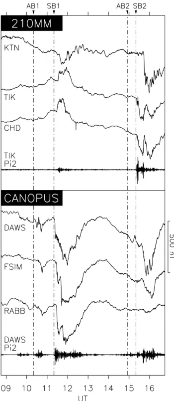
The interval of study is 09:00 to 16:30 UT on 5 June 1998. During this interval, the Ultraviolet Imager (UVI) instrument on board the Polar satellite (Torr et al., 1995) was imaging al-most the entirety of the Northern Hemisphere auroral zone, giving continuous information regarding the size of the po-lar cap. In addition, six Super Dual Auroral Radar Network (SuperDARN) radars (Greenwald et al., 1995) were provid-ing convection flow measurements in the dayside ionosphere, that region in which dayglow makes measurement of the au-rora difficult for the UVI imager. The combination of these two data sets allows for the OCB to be monitored at nearly all local times. Finally, overpasses of the Defense Mete-orological Satellite Program DMSP F13 and F14 satellites (Hardy et al., 1984), the National Oceanographic and At-mospheric Administration NOAA-12 satellite (Raben et al., 1995), and the Fast Auroral SnapshoT (FAST) spacecraft (Carlson et al., 1998) provide auroral particle measurements which allow the OCB to be identified without ambiguity, and in effect calibrate the UVI and SuperDARN measurements. Two substorms occurred during the interval of interest, the progress of which were monitored by six magnetometer sta-tions from the 210 Magnetic Meridian (210MM) network (Yumoto, 1996) and the Canadian Auroral Network for the OPEN Program Unified Study (CANOPUS) network (as de-scribed by Samson et al., 1992). These stations are KTN, TIK, and CHD (210MM) and DAWS, FSIM, and RABB (CANOPUS). Upstream solar wind and IMF conditions were monitored by the Wind and ACE spacecraft.
Fig. 3. H -component magnetograms from the 210MM and
CANO-PUS networks, along with filtered data showing Pi2 activity (scaled by a factor of 5 for clarity). Vertical dot-dashed lines are the same as Fig. 2.
2.1 Overview
Polar UVI images were acquired with the LBH-long filter every 37 s. These observations are summarized in Fig. 2a–c, which show latitude-time-intensity plots of the auroral
lumi-nosity measured along the 18, 00, and 06 MLT meridians. At the start of the interval, before approximately 12:00 UT, a band of luminosity is seen to progress gradually equator-wards, especially along the 06 and 18 MLT meridians. Dur-ing this period, two minor auroral brightenDur-ings are observed along the 00 MLT meridian, the most significant of which started at 10:20 UT, which we will refer to as “auroral bright-ening 1” (AB1). At 11:20 UT another intensification of the auroral luminosity at 00 MLT signifies substorm expansion phase onset, “substorm breakup 1” (SB1). This luminosity broadens considerably at 11:40 UT and a poleward motion of the lower latitude boundary of the luminosity becomes appar-ent. The auroral substorm bulge is seen to progress to earlier and later local times, crossing the 06 and 18 MLT meridi-ans at 11:55 and 12:05 UT, respectively. Following this there is a poleward retreat of the auroral luminosity, which also dims with time, until 14:00 UT when it has almost disap-peared entirely, except along the midnight meridian. After this time, however, it is clear that the auroral band is mov-ing equatorwards once again. Finally, at 15:20 UT the aurora intensifies once again, again signifying substorm onset. Ex-amination of auroral images at all local times indicates that the auroral brightening (“auroral brightening 2”, AB2) actu-ally commences in the post-midnight sector, some time close to 14:55 UT, followed by a major intensification in the pre-midnight sector at 15:20 UT, “substorm breakup 2” (SB2).
Figure 3 shows H -component magnetograms from three 210MM stations located in the pre-midnight sector and three CANOPUS stations located in the post-midnight sector. The locations of these stations are shown in Fig. 4 as red dots, cor-responding, from west to east, to TIK, KTN, CHD, DAWS, FSIM, and RABB. At the start of our interval the CANO-PUS stations are located closest to midnight, and hence, it is these stations which observe the first substorm (SB1) bay and associated Pi2 signature most clearly (11:20 UT). Prior to this, at 10:20 UT, there is also evidence of a small bay and some Pi2 activity associated with the first auroral brighten-ing (AB1). As time passes and the stations progress to later local times, the 210MM stations approach midnight and it is here that the second substorm (SB2) bay and Pi2 are most clearly observed (15:20 UT). It is interesting to note that the auroral brightening (AB2) prior to this at 14:55 UT does not have a clear signature in the magnetograms (except maybe at DAWS), but this is perhaps because the auroral activity takes place in the gap between the two magnetometer net-works. The times of these auroral features, AB1, SB1, AB2, and SB2, are indicated by vertical dot-dashed lines in both Figs. 2 and 3.
Latitude-time plots of Doppler velocity measured by the Kapuskasing and Goose Bay radars, beams 12 and 6, re-spectively, are shown in Fig. 2d and e. Between 09:00 and 16:30 UT these two radars progress from the dawn sector to the noon sector. Radar echoes are not observed at all times or latitudes, but are dependent on the presence of irregularities in the ionosphere from which to backscatter (for a discus-sion, see Milan et al., 1997). Indeed, the occurrence of iono-spheric irregularities, and hence, radar backscatter, often
ap-(a–b)
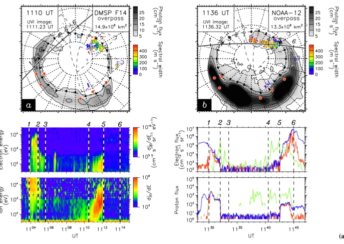
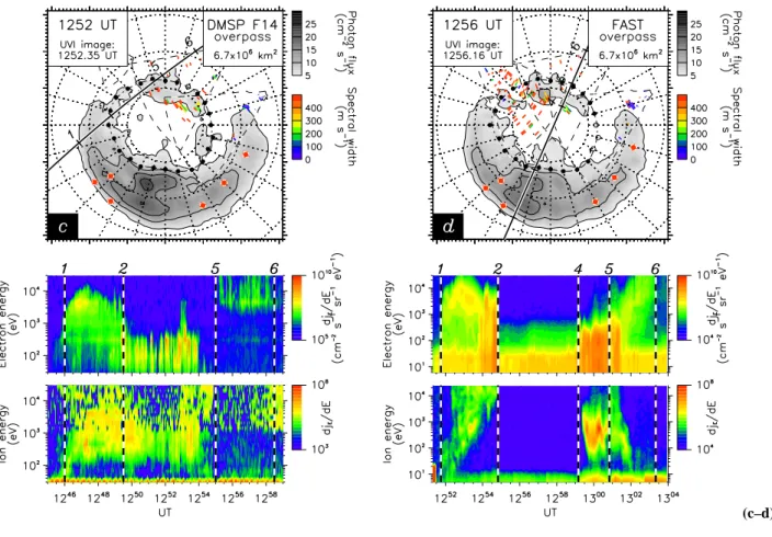
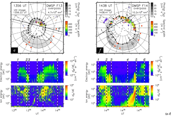
Fig. 4. (Upper panels) Composite plots of the Polar UVI auroral luminosity (grey scale) and radar spectral width (colour scale) on magnetic
latitude and MLT coordinates. Dotted circles represent 60◦, 70◦, and 80◦latitudes and radial dotted lines represent MLT meridians, 12 MLT being directed towards the top of the panel. Dashed lines show the fields-of-view of the radars. Filled dots indicate estimates of the OCB latitude at each MLT meridian, open dots showing interpolated points in regions where no observations are available. The dot-dashed line is a somewhat smoothed fit to these points (see text for details), i.e. indicates a rough estimate of the location of the OCB. Superimposed is the track of the overpassing spacecraft, tick marks indicating the locations of boundaries 1 − 6 identified in the lower panels. Red dots mark the locations of magnetometers employed in the study: from west to east, TIK, KTN, CHD, DAWS, FSIM, and RABB. (Lower panels) Electron and ion measurements from the overpassing satellite. In the case of DMSP F13 and F14 and FAST, these are spectrograms between
∼10 eV and 30 keV. In the case of NOAA-12 these are fluxes of > 30 keV electrons and ions at two pitch angles – 10◦(i.e. precipitating; red lines) and 80◦(i.e. trapped; blue lines) – and ∼100 eV particles mainly of magnetosheath origin (green lines). These latter fluxes have been reduced by a factor of 103for plotting purposes. From these observations, six boundaries have been identified, 1 and 6 being the approximate equatorward boundary of precipitating trapped particles, 2 and 5 the poleward edge of this region, i.e. the trapping boundary, our proxy for the OCB, and 3 and 4 the approximate poleward edge of the magnetosheath precipitation.
pears to delineate important magnetospheric boundaries (Mi-lan et al., 1998), and in the present study it is the equatorward edge of the main region of backscatter, corresponding to the spectral width boundary, as discussed in the Introduction, on which we will concentrate below. For the time being we note that the Goose Bay radar observes scatter throughout most of the interval, and the latitudinal variation in the location of this scatter qualitatively follows the auroral observations described above, i.e. there is little motion of the backscat-ter prior to 11:30 UT, followed by a poleward progression until 13:30 UT. After this time the scatter moves equator-ward once again, until a poleequator-ward retreat some time after 16:00 UT. The Kapuskasing radar observes backscatter only after 13:30 UT, but here again this is dominated by an equa-torward motion until 16:20 UT, after which the backscatter
retreats polewards.
Figure 2f and g indicate the Byand Bzcomponents of the
IMF as measured by both the ACE (thin line) and Wind (thick line) spacecraft, lagged to the magnetopause by the estimated solar wind propagation delay (66 and 78 min, respectively). Figure 2h shows the corresponding IMF clock angle, defined as θ = atan (Bz, By). In general, an extremely good
agree-ment is found between both solar wind monitors, giving con-fidence that we are able to characterize the incoming IMF orientation with accuracy. For the purposes of the present study we can say that IMF Bywas approximately −5 nT for
the duration of the interval of interest. The Bx component
(not shown) varied slowly between 0 and 3 nT throughout most of the interval. The Bz component of the IMF, the
(c–d)
Fig. 4. Continued ...
the solar wind and magnetosphere on the dayside, varies be-tween positive and negative throughout the interval, but does so in a series of sharp transitions, especially after 11:00 UT. Four sub-intervals can be identified in which Bzis
predom-inantly negative: 09:00–10:00 UT, 10:20–11:15 UT, 12:15– 12:30 UT, and 13:50–15:30 UT. By way of a first compari-son between these IMF observations and the auroral observa-tions, we note that the last of these sub-intervals in which Bz
is negative, suggesting that dayside low-latitude reconnec-tion should be ongoing, is associated with an equatorward motion of the aurora observed by UVI and backscatter ob-served by SuperDARN. Conversely, backscatter and aurora are observed to retreat polewards when Bz is positive and
substorm activity is pronounced (11:30–13:00 UT and after 16:00 UT).
2.2 Identification of the polar cap boundary
We have seen that features in auroral and radar observa-tions appear to move equatorward or poleward in response to changes in the IMF or the occurrence of substorms. In the next section, we employ satellite particle observations to determine which auroral and radar features give a good indi-cation of the loindi-cation of the OCB, to allow us to estimate the area of the polar cap. The FAST, DMSP and NOAA satel-lites overpass the northern polar regions thirteen times
dur-ing this interval, marked at the top of Fig. 2. We cannot show the details of all of these overpasses, and so we concentrate on the six most representative. Figure 4 presents compos-ite diagrams of the UVI, SuperDARN, and FAST, DMSP or NOAA data sets for each of these six overpasses. The up-per panels show a UVI image in magnetic latitude and MLT coordinates from a time close to the middle of the overpass and the backscatter observed simultaneously by the (in or-der from west to east) Kapuskasing, Goose Bay, and Han-kasalmi radars of the SuperDARN chain. The fields-of-view of these radars are indicated by dashed lines. Three other Northern Hemisphere radars are also making measurements at these times, Saskatoon, Stokkseyri, and Pykkvibær, but for clarity these data are not shown, as their fields-of-view overlap with those already presented. Backscatter is only shown where significant return power is observed, and this backscatter is colour-coded with the spectral width of the re-turn echoes. The UVI images have been processed to remove the dayglow. Unfortunately, dayglow swamps weak auroral emissions from the dayside and little luminosity is observed near noon, especially towards the end of our interval when the geomagnetic pole is rotated towards the Sun.
The lower panels show the electron and ion characteristics observed by the overpassing satellite. Both DMSP and FAST observations are presented as spectrograms: in the case of DMSP F13 and F14, these cover the energy range 30 eV to
(e–f)
Fig. 4. Continued ...
30 keV, in 18 energy channels; the FAST spectrograms show particle fluxes between energies of 5 eV and 30 keV, in 47 energy channels. In the case of NOAA-12 these are fluxes of “trapped” > 30 keV electrons and ions at two pitch an-gles – 10◦ (i.e. precipitating; red lines) and 80◦ (i.e.
mir-roring just below the spacecraft; blue lines) – and ∼100 eV particles (green lines). It is these particle observations that we employ to identify the OCB, which we then generalize to all local times using the UVI and SuperDARN observa-tions as a guide. In particular, the OCB signature we look for is a sharp demarcation between high and low fluxes of high energy (> few keV) particles. These high energy par-ticles are generally considered to be present on closed field lines only, as such particles cannot persist for long on open field lines. In each overpass the occurrence of this signature as the satellite passes into and then out of the polar cap is marked by the numbers 2 and 5. Four other boundaries are also marked for interest. The first pair represent the approx-imate low-latitude boundaries of the high energy particles (1 and 6). In addition to the high energy particles, low energy precipitation is also observed. Significant fluxes of low en-ergy (< 1 keV) electrons can be observed poleward of the OCB, and on the dayside this precipitation is considered to be of magnetosheath origin. In such regions, dispersed ion signatures (few eV–10 keV) can also be found, a character-istic of very recently reconnected field lines, as will be
dis-cussed in more detail below. The approximate high latitude extremes of this precipitation region are indicated by bound-aries 3 and 4. Poleward of this, a low flux of very low en-ergy (∼100 eV) electrons is indicative of polar rain on open field lines. The points at which these boundaries are crossed along the satellite track are indicated in the top panels by tick marks. As will be described below, in each overpass we find gratifying consistency between the observations of all three techniques.
We turn first to the DMSP F14 overpass of 11:10 UT (Fig. 4a). As the satellite crosses the dusk auroral oval, the region of high energy precipitation on closed field lines is found to coincide with the peak in UV luminosity (1 − 2). Lower luminosity emission is seen just poleward of this, and this is associated with low energy electron precipitation on recently opened field lines (2−3). As the satellite approaches the noon sector OCB a dispersed ion feature is observed, in which ion energy decreases with increasing latitude (4 − 5). Such features are characteristic of precipitation on newly-reconnected field lines for southward IMF (e.g. Reiff et al., 1977; Woch and Lundin, 1992), with the dispersion being a consequence of the velocity filter effect. The sharp lower-latitude cutoff of this ion feature marks the OCB, and though high energy electrons are observed equatorward of this, they are of extremely low flux. No luminosity is observed in con-junction with this traversal of the auroral zone, as here the
aurora are swamped by dayglow. Backscatter is observed in the pre-noon sector by the Goose Bay radar at this time. In the equatorward portion of this backscatter the spectral widths are high, and it is the equatorward edge of this re-gion of backscatter which we associate with the OCB. As expected, this equatorward edge of the backscatter is found to line up with the poleward edge of the auroral oval in the dawn sector, and a similar association can be seen in both dawn and dusk sectors in Fig. 4f, another period of south-ward IMF. This association between the backscatter and the OCB appears to break down at other times, when the IMF is directed northwards, as we will see below.
Using the signatures of the OCB which we have identified, i.e. the poleward boundary of high energy precipitation, the poleward gradient in the UVI auroral intensity, and the equa-torward boundary of high spectral width radar backscatter, it is possible to estimate the location of the OCB at most local times. This is shown along each MLT meridian as a dot. The dots are solid if there are observations within that MLT sec-tor which identify the OCB latitude. If no nearby signature is found, the OCB latitude is interpolated from earlier and later MLTs, and this is shown by open dots. The area of the polar cap is then easily calculated by numerically integrating the size of each MLT sector, and this area is shown in the top right of each panel. While we realize that this determi-nation of the polar cap area, Apc, is only approximate, we
find that the error introduced by assuming that our estimate of the boundary latitude is off by +1◦ at all MLTs, or off by −1◦at all MLTs, is only of the order of ±10%. As will be discussed below, we are primarily interested in relative changes in area, and so as long as our boundaries have been estimated consistently, these errors have a negligible impact on our conclusions.
Finally, mainly for illustrative purposes, though this will be of use later, an approximate OCB is shown by a dot-dashed line in each panel. The fit is achieved by determining the Fourier transform of the OCB latitude as a function of MLT and then using the first six terms as a series expansion to represent the boundary. This order of fit was found to be a good compromise between representing our boundary esti-mates with accuracy without introducing spurious “wiggles”, especially on the dayside where this fit will be used later on. The above discussion for Fig. 4a, an overpass during which IMF Bz < 0 nT, is equally valid for the other
IMF southward pass shown in Fig. 4f. At this time, radar backscatter is observed across almost the entirety of the day-side boundary, between 06 and 18 MLT. Later, we will em-ploy this coverage to estimate the dayside reconnection volt-age. However, for now we note that this allows us to esti-mate the location of the dayside OCB with accuracy, even where no auroral luminosity is seen. The relationship dis-cussed above between the equatorward boundary of the radar scatter and the OCB is confirmed in this overpass as the satellite tracks directly overhead the radar fields-of-view. In-deed, there appears to be a close correspondence between radar backscatter and precipitation of magnetosheath origin on open field lines, that is between boundaries 2 − 3 and
4 − 5. In addition, a distinct dispersed ion signature is seen by DMSP F14 as it traverses the radar backscatter near noon. A slightly different story is found during intervals of north-ward IMF, that is Fig. 4b–e. At these times significant but low level auroral luminosity appears within the polar cap poleward of the OCB, co-located with the magnetosheath precipitation on open field lines (boundaries 2 − 3 and 4 − 5) on the dayside. We assume that the OCB is co-located with the equatorward edge of this luminosity. In Fig. 4d this lu-minosity feature displays a distinct enhancement near local noon, similar to that found by Milan et al. (2000a) and Frey et al. (2002), who identified this as a signature of high-latitude reconnection. Indeed, the close approach of the FAST space-craft to this auroral region shows a distinct reversed cusp ion dispersion at its poleward edge, that is ion energy falling with decreasing latitude, again a signature of high-latitude recon-nection (Woch and Lundin, 1992). At these times of north-ward IMF the radar backscatter no longer appears to define the OCB with any accuracy, especially near noon, as was found by Moen et al. (2001). There is some suggestion, how-ever, that when backscatter is present it lies close to the pole-ward edge of the high-latitude luminosity region (Figs. 4b, c and e).
On the nightside, the main auroral oval is most luminous in Fig. 4b, as this is the expansion phase of the first sub-storm (SB1), but decreases markedly in brightness through to Fig. 4e. It is only after the subsequent southward turn-ing of the IMF (Fig. 4f) and onset of the second substorm (not shown) that the low-latitude, nightside auroral luminos-ity begins to increase to its original levels. The one satellite overpass of the nightside auroral zone that is available to this study, that of the FAST spacecraft at 12:56 UT (Fig. 4d), in-dicates that the poleward edge of the auroral bulge of SB1 (which should map to reconnection site e in Fig. 1) is co-located with the loss of high energy electrons and ions; pole-ward of this the particle characteristics are indicative of open field lines. Weak auroral emission is present poleward of the OCB at this time, though the origin of this is not clear since the weak, soft precipitation observed inside the po-lar cap should not generate significant luminosity. More noon-midnight satellite passes would be necessary to fully determine how the nightside auroral emission relates to the location of the OCB, especially during periods when the nightside reconnection site is not active. In the absence of more concrete evidence, and following the FAST overpass of Fig. 4d, we have placed the OCB at the maximum in the gra-dient of the UVI intensity at the poleward edge of the night-side auroral oval. We feel that our uncertainty in the location of the nightside OCB contributes most significantly to any er-ror in our estimation of the polar cap area. To counteract this, as discussed above, we have attempted to be as consistent as possible in our boundary identification.
In summary, Fig. 5 presents a schematic showing the most important particle, UV aurora and radar backscatter features which we have identified above, and their relationship to the OCB, under southward and northward IMF conditions and non-substorm intervals (no reconnection at point e in Fig. 1).
~10 keV ions and electrons <1 keV electrons Dispersed ions Strong UV aurora Weak UV aurora
IMF B
z< 0 nT
UV aurora <1 keV electrons Reverse-dispersed ions ~10 keV ions and electronsIMF B
z> 0 nT
Open/closed boundary Low latitude merging gap High latitude merging gap Open/closed boundary Radar backscatter poleward of merging gapBackscatter equatorward of merging gap UV aurora
Fig. 5. A schematic diagram illustrating the main signatures
em-ployed to identify the OCB (thick solid line) and their relationship to the dayside merging gap (thick broken line) and convection flow, for IMF northwards and southwards. Panels to the left indicate the UV and radar auroral regions. Precipitating particle characteristics and convection streamlines are shown to the right.
To the left, radar and auroral features are shown, and on the right particle signatures are indicated along with our expec-tation of the convection flow associated with low- or high-latitude reconnection; for simplicity, we have neglected the influence of IMF Byon the convection streamlines. For both
northward and southward IMF cases, the dayside OCB maps to point a in Fig. 1. For southward IMF, reconnection occurs at a and the merging gap maps to the OCB. During north-ward IMF, however, reconnection occurs at high latitudes, near b, and as a consequence the ionospheric projection of the merging gap is located within the polar cap. In both cases magnetosheath-like precipitation and dispersed ion sig-natures are observed on field lines that have recently crossed the merging gap; as a consequence of the directions of con-vection flow in each case, magnetosheath precipitation coats the poleward edge of the dayside OCB. High energy precip-itation on closed field lines appears at all local times, though the UV aurora associated with this tend to be weaker on the dayside, especially where dayglow dominates. During north-ward IMF and after substorm activity has died away the main UV oval becomes faint and confined to the nightside.
2.3 Variations in polar cap area
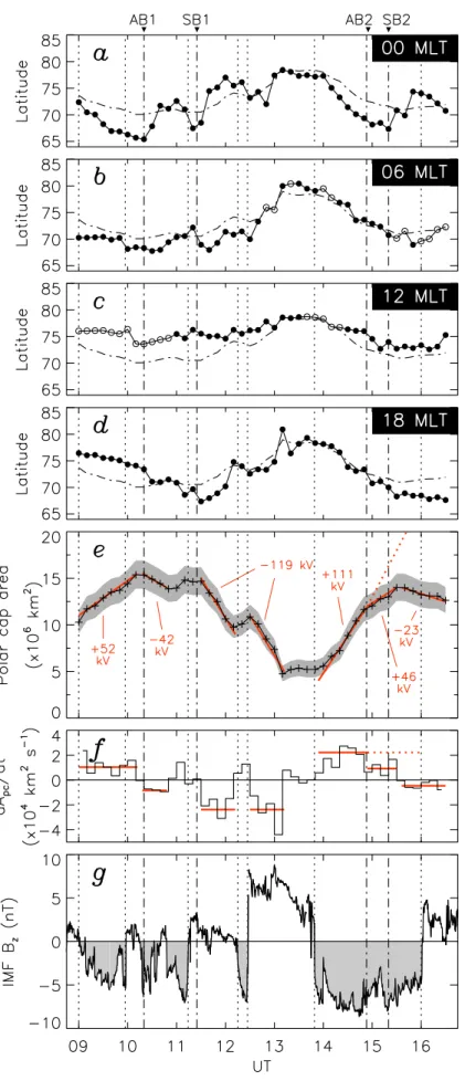
The thirteen satellite overpasses described in the previous section allow for the OCB to be extrapolated to all local times, based on the supporting radar and auroral observa-tions. Between each pass, the same radar and auroral sig-natures can be used to identify the location of the OCB, even when particle data are not available. In this way, the loca-tion of the OCB and the area of the polar cap have been determined every 10 min throughout the interval 09:00 to 16:30 UT. Figures 6a–d show time series of the latitude of the OCB as determined along the dawn, dusk, noon and mid-night meridians. Filled circles show where the OCB latitude was determined from a nearby particle, auroral or radar sig-nature, whereas open circles show points which were inter-polated (as discussed in relation to Fig. 4). Figure 6e shows the polar cap area, Apc, determined from the boundary
iden-tifications. The grey region shows the uncertainty in the de-termination of Apc, in the limits that the latitude of the OCB
was over- or underestimated by 1◦ of latitude at all local times. As suggested by Eq. (1), the rate of change the of po-lar cap area is related to the difference between the day- and nightside reconnection rates, so dApc/dtis shown in Fig. 6f.
Figure 6g shows the Bz component of the IMF, time-lagged
to the magnetopause. Vertical dotted lines show when Bz
changed markedly, usually a transition from positive to neg-ative, that is IMF northward to southward, or vice versa, as discussed in Sect. 2.1. The vertical dot-dashed lines show the onsets of the auroral brightenings and substorm breakups, also indicated in Figs. 2 and 3.
First, we discuss the variations in the polar cap area. At the start of the interval, the IMF is oriented southward, sug-gesting that low-latitude dayside reconnection should be cre-ating new open flux, and indeed the area of the polar cap increases between 09:00 and 10:15 UT. Following the onset of the first auroral brightening (AB1), the polar cap shrinks between 10:20 and 10:50 UT, indicating that reconnection in the magnetotail is destroying open flux. There is a brief re-covery of the polar cap area between 10:50 and 11:05 UT, suggesting that tail reconnection has ceased and dayside re-connection is still ongoing as the IMF is directed southwards. Thereafter, the IMF turns northward, suggesting a cessation of dayside reconnection, and the polar cap area remains uni-form until ∼11:30 UT. At this time the first substorm breakup (SB1) occurs, and we might expect the polar cap to shrink as nightside reconnection commences. This is found to be the case, with the polar cap shrinking rapidly from some 1.5 × 10⁷km2 to close to 0.5 × 10⁷km2, that is to a third of its initial size, over the next 100 min. There is a short pe-riod during this interval, between 12:15 and 12:30 UT, when the IMF turns southward once again, and at this time the polar cap area recovers somewhat. This is, however, only a brief pause during the ongoing polar cap shrinkage. At 13:10 UT the decrease in the polar cap area associated with SB1 ceases. This time corresponds approximately to the end of the recovery phase of the substorm, as determined from the magnetogram of, say, FSIM (Fig. 3), i.e. magnetotail
recon-Fig. 6. (a–d) Time series of the OCB
latitude along the noon and midnight, dawn and dusk meridians. The latitude of the equivalent circular OCB (ECB) is indicated by a dot-dashed curve. (e) The area of the polar cap deduced from the OCB estimates (crosses), the grey area indicating the uncertainty based on assuming our OCB estimate is incorrect by ±1◦at all local times. Superimposed in red are lines approximating the vari-ation in polar cap area. The numbers are estimates of 8day−8night. (f) The rate of change of area of the polar cap. Red lines indicate the gradients of the fits shown in panel (e). (g) The IMF
Bzcomponent, time-lagged to the
mag-netopause. In all panels, vertical dot-ted lines indicate the times of transitions in IMF Bzand vertical dot-dashed lines
indicate the onsets of substorm breakup and auroral brightening.
nection appears to continue from substorm expansion phase onset to the end of the recovery phase, an interval of over an hour and a half. A similar finding was reported by Khan et al. (2001), in which reconnection signatures were observed in the magnetotail some time after significant auroral activ-ity had subsided. After 13:10 UT, the area of the polar cap area remains constant. It is not until the southward turning of the IMF at 13:50 UT that dayside reconnection recommences and the polar cap expands. At ∼14:55 UT the IMF continues to be directed southwards, but the rate of expansion of the polar cap is diminished, this time corresponding to the sec-ond auroral brightening (AB2). This slowing of the polar cap expansion indicates that magnetotail reconnection is de-stroying open flux, though not as quickly as new open flux is being created on the dayside. After 15:20 UT, the onset of the second substorm (SB2), the polar cap begins to shrink, suggesting that the closure of open flux in the magnetotail now dominates over the ongoing creation of open flux on the dayside.
At times when the polar cap is expanding or contract-ing, the rate of change of area appears relatively uniform, as shown by fits-by-eye to the variation in Apc shown in
Fig. 6e; the rate of change of the area represented by these fits is also indicated in Fig. 6f. The gradient of these fits is related through Eq. (1) to the difference in the day- and night-side reconnection voltages. During the first substorm growth phase, prior to AB1, when IMF Bz ≈ −4 nT, the fit to the
polar cap growth rate indicates that 8day−8night ≈52 kV.
If we assume that no nightside reconnection is occurring at this time, i.e. 8night ≈ 0, then 8day ≈ 52 kV.
Simi-larly, during the growth phase of the second substorm, when
Bz ≈ −7 nT, we can estimate that 8day ≈ 111 kV prior
to AB2. Two recent studies of the growth rate of the po-lar cap during southward IMF estimated 8day ≈160 kV for
Bz ≈ −10 nT (Milan et al., 2000b) and 8day ≈ 48 kV for
Bz≈ −4 nT (Milan and Lester, 2001). Taken together, these
values suggest that the rate of reconnection on the dayside is dependent on the magnitude of the southward component of the IMF, with 8day ≈15|Bz|kV, where Bz is expressed
in nT and Bz <0 nT. This relationship is similar to the
sta-tistical findings of Yeoman et al. (2002), who suggested that
8day≈20|Bz|kV.
During the first substorm expansion and recovery, the de-crease in polar cap area indicates that 8day −8night ≈
−119 kV. If we assume that no low-latitude dayside re-connection is occurring during these intervals as the IMF is oriented northward, that is 8day = 0, then 8night ≈
119 kV. After the onset of AB2, the expansion associated with the second substorm growth phase is slowed, such that
8day−8night ≈46 kV. However, the IMF does not change
markedly at this time, so we assume that the dayside re-connection voltage remains unchanged at 8day ≈ 111 kV
(hence, the dotted fit in Fig. 6e), giving a nightside reconnec-tion voltage of 8night≈65 kV. After substorm breakup SB2,
8day−8night ≈ −23 kV; if the dayside reconnection rate
is again assumed to remain undiminished, this indicates that
8night ≈134 kV. We see, then, that the rate of reconnection
on the nightside during the auroral brightening AB2 (65 kV) is only half of that ongoing during the expansion phases of the two substorms (111 and 134 kV, respectively). The sit-uation is not so clear following AB1, as the IMF is highly variable at this time, so it is difficult to estimate 8day.
As suggested above, when the IMF is directed northwards and no substorm-associated reconnection is ongoing, within intervals 11:05–11:30 and 13:10–13:50 UT, the area of the polar cap remains constant. This suggests that open flux is not closed by high-latitude reconnection at these times; in-stead, we anticipate that lobe-stirring, a circulation of the open flux, is excited (see also our schematic in Fig. 5). Clo-sure of open flux is only expected if individual interplanetary magnetic field lines reconnect with both northern and south-ern lobes (e.g. Cowley, 1981), a situation that should only arise if the IMF has no significant Bycomponent; this is not
the case during the present interval.
Examination of Fig. 6a–d reveals, as might be expected, that the response of the OCB to changes in polar cap area was not uniform at all local times. One of the motivations of the present study was to examine how well the OCB latitude in different MLT sectors characterizes the OCB at all local times, i.e. if observations of the OCB are available at one lo-cation only, and the polar cap is assumed to be circular, how accurate is the estimate of the polar cap area. To this end, su-perimposed on each panel is a dot-dashed line representing the latitude of the boundary of a circular polar cap, centred on the geomagnetic pole, of equivalent area to the simultane-ous estimate of Apc. In effect this shows how distorted the
polar cap is from a circle, and how far its centre is shifted from the pole. In the noon sector the OCB is generally found at a higher latitude than the equivalent circular OCB (which we will refer to as the equivalent circular boundary or ECB). Moreover, the range of latitudes over which the noon OCB moves (∼5◦) is much less than would be the case for a cir-cular polar cap (∼10◦). In the midnight sector the boundary moves much more rapidly than the leisurely meanderings of the noon OCB, and is sometimes equatorward (usually prior to substorm breakup), or sometimes poleward (during sub-storm breakup) of the ECB. Indeed, while the noon OCB moves only slowly with time, the midnight OCB responds rapidly to the onset of dayside coupling or substorm breakup. The dawn and dusk OCBs are found to match the ECB rela-tively closely, especially after 11:00 UT.
These results are shown in another format in Fig. 7a–d. Here, the latitude of the OCB along each of the four merid-ians is plotted as a function of polar cap area. The dotted curve superimposed on each panel shows the ECB latitude as a function of Apc, which, by definition, is the same at all
local times. Least-squares fits between the OCB latitude 3 and Apcare shown by solid lines and quantified at the bottom
of each panel. Perhaps unsurprisingly, the smallest spread is found in the noon sector, though here a point measurement of the latitude of the OCB, extrapolated to all local times, would, in general, lead to an underestimate of the polar cap area. The large spread along the midnight meridian is due to the large and rapid motions of the OCB in response to
sub-Fig. 7. (a–d) The latitude of the OCB as a function of polar cap area along the dawn and dusk, noon and midnight meridians. Linear fits
to the variations are indicated by solid lines, and the fit quantified at the bottom of each panel. The latitude of the equivalent circular OCB (ECB) is shown by the dotted lines. (e) and (f) The displacement of the centroid of the polar cap from the geomagnetic pole, expressed as degrees of latitude along the noon-midnight and dawn-dusk meridians. Positive displacements are towards noon and dusk, respectively.
storm phenomena. A large spread is also found along the dusk and to a lesser extent the dawn meridians, mainly as a consequence of the overall shift of the polar cap towards dawn or dusk that will be described below. Interestingly, at small polar cap areas the OCB in each local time sector ap-proaches the ECB, i.e. the smaller the polar cap, the more circular and centred on the geomagnetic pole it becomes. Figure 7e–f show the displacement of the centroid of the po-lar cap from the geomagnetic pole, along the noon-midnight and dawn-dusk meridians, respectively, as a function of UT; here, displacements towards noon and dusk are positive. It is found that on average, the centroid of the polar cap is dis-placed from the pole towards the nightside by of the order of 1◦ of latitude, consistent with previous reports. There is
a significant variation in the displacement, however, gener-ally between the values of 0◦ and 2◦. The centroid appears to move towards the nightside during the substorm growth phase (09:00 to 10:00 UT and 13:30 to 14:50 UT), and
re-turns towards the pole following significant nightside auro-ral activity (following each auroauro-ral brightening and substorm breakup). Along the dawn-dusk meridian there is also a sig-nificant displacement, towards dawn prior to 11:00 UT and towards dusk after 15:00 UT. It might be expected that such a shift is caused by the east-west component of the IMF (e.g. Cowley et al., 1991) and yet Byis negative during both these
intervals.
2.4 Estimating the dayside reconnection voltage from radar measurements
As suggested in the Introduction, the day- or nightside recon-nection voltages can, in principle, be directly estimated from measurements of the convection flow across the open/closed field line boundary. This is not possible throughout most of the interval of study, as the radar backscatter coverage is not sufficient. However, after 14:00 UT radar backscatter is
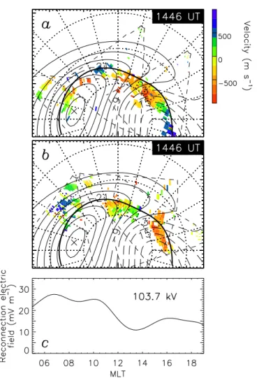
ob-Fig. 8. (a) The line-of-sight plasma
drift velocities deduced from the radar observations at 14:46 UT, during the growth phase of the second substorm. Positive and negative velocities are towards and away from each radar, respectively. Radars (west to east) Kapuskasing, Goose Bay and Han-kasalmi are shown. Superimposed are contours of the electrostatic potential (solid/dashed lines are negative/positive potentials with a contour interval of 6 kV) inferred from the line-of-sight ve-locities (see text for details). Also indi-cated is the location of the OCB (solid line) determined from the equatorward edge of high spectral width backscat-ter. (b) Similar to panel (a), though
showing the radar observations from the (west to east) Saskatoon, Stokkseyri, and Pykkvibær radars. The potential so-lution and OCB are the same in (a) and (b). (c) The reconnection electric field determined from the plasma drift per-pendicular to the OCB. The integral of this along the boundary between 05 and 19 MLT is shown in the top right-hand corner.
served at almost all local times between 06 and 18 MLT (see, for example, Fig. 4f), and hence, an estimate of the dayside reconnection voltage can be made. Below, we employ these radar measurements of the convection flow, in conjunction with our knowledge of the motion of the OCB, to estimate the dayside reconnection voltage during the growth phase of the second substorm, and compare this with our previous es-timate of ∼111 kV determined from the rate of growth of the polar cap, for which estimate we assumed that no nightside reconnection was taking place.
Figure 8 shows the line-of-sight plasma drift estimates made by the Northern Hemisphere SuperDARN radars at 14:46 UT. This time was selected for illustration as it is typ-ical of the observations made during the growth phase of the second substorm. For the sake of clarity, the observa-tions are shown in two separate panels: panel (a) contains the measurements from the three radars included in Fig. 4, whereas panel (b) shows their corresponding radar twins. Positive and negative velocities correspond to flow towards and away from each radar, respectively. A thick line indi-cates the location of the OCB, estimated from the equator-ward edge of high spectral width radar backscatter, as dis-cussed previously. To determine the dayside reconnection voltage, it is necessary to integrate the reconnection electric
field at all points along this boundary, which is given by the component of plasma drift perpendicular to the boundary. To construct the two-dimensional flow pattern from the line-of-sight velocities, from which the reconnection electric field can be estimated, we employ the analysis technique devel-oped by Ruohoniemi and Baker (1998). This technique de-termines the solution for the distribution of electrostatic po-tential expressed as a series expansion in spherical harmon-ics (in our case, of order of 6), constrained by the line-of-sight measurements of the radars. Contours of the electro-static potential so derived are superimposed on Fig. 8a and b, which in effect represent convection flow streamlines. In regions where no radar backscatter is present the potential solution is driven by a statistical convection model, which may not accurately reflect the instantaneous flows occurring in the ionosphere. However, in regions where backscatter is present, thus constraining the solution, the contours repre-sent a flow pattern that accurately reflects the line-of-sight measurements. The great advantage of this technique is that, since the solution is an analytic function, the potential or electric field can be calculated at any arbitrary location, un-limited by the spatial resolution or occurrence of the radar backscatter. This makes the determination of the boundary-parallel electric field (boundary-normal plasma drift) at all
points along the boundary extremely straightforward. This gives us the reconnection electric field in the Earth’s frame, but we are really interested in the electric field in the bound-ary’s rest frame, so we must take the motion of the boundary into account. It is here that the largest uncertainty enters our calculations, as determination of the instantaneous boundary velocity is difficult. However, this can be interpolated from the motion of our boundary identifications, and from this we find the boundary speed to be close to 160 m s−1 (represent-ing an electric field of 8 mV m−1) along most of its length in the MLT range of interest. The variation with MLT of the sum of the convection and boundary motion contributions to the reconnection electric field is shown in Fig. 8c. The re-connection voltage is the integral of the rere-connection electric field, and between 05 and 19 MLT this is found to be 104 kV, in good agreement with the estimate of 111 kV from the rate of growth of the polar cap at this time. As mentioned above, the estimate of the boundary motion speed is the largest un-certainty factor in this calculation: an increase of 10 m s−1in the speed of the equatorward motion of the boundary would increase the estimate of the dayside reconnection voltage by 2.5 kV. In addition, there may be a small additional contri-bution to the dayside reconnection voltage from earlier and later local times than those considered, but insufficient radar coverage does not allow us to quantify this.
The electric field measurements themselves are of inter-est. It is clear from Fig. 8c that the reconnection electric field maximizes in the pre-noon sector, between 06 and 12 MLT, consistent with the prevailing IMF orientation, that is By < 0 nT. We can consider this to be the convection
throat, and indeed it is in this region that the most mani-fest signatures of bursty reconnection are observed, as will be described in Sect. 2.5. In addition, the closest satellite overpass (Fig. 4f) shows a dispersed ion signature in this local time sector. However, the electric field remains non-zero at all points along the boundary considered, from which we can deduce that reconnection is taking place at most lo-cal times along the dayside magnetopause. This is consis-tent with the observation of magnetosheath-like precipitation along all dayside portions of the OCB sampled by the over-passing satellites (see also Fig. 5). That reconnection can ex-tend to the flanks of the magnetopause has previously been suggested by Milan et al. (2000b), who showed ionospheric reconnection signatures extending from noon to 18 MLT for
By > 0 nT, and the observations of Kawano and Russell (1996) which show magnetopause reconnection signatures as far tailwards as X = −10 RE.
Much of the flow crossing the OCB has a large sunward component, especially in the post-noon sector, placing the convection reversal boundaries (or focii of the twin-cell po-tential pattern) within the polar cap, possibly contrary to expectations. However, this picture is consistent with the paradigm of Lockwood (1997), in which the merging gap is suggested to be located at lower latitude and to be much broader in MLT extent than previous estimates based on “tra-ditional” interpretations of low altitude particle precipitation cusp signatures (e.g. Newell and Meng, 1992). Indeed, there
is considerable similarity between our Fig. 8 and Fig. 1b of Lockwood (1997). If anything, the paradigm of Lockwood would suggest that the true location of the OCB might lie a small distance equatorwards of our estimate, as no signa-tures of the coupling taking place at the magnetopause can reach the ionosphere in less than one Alfv´en travel-time, of the order of 1 or 2 min, in which time magnetic field lines threading this region have convected some distance pole-wards (see, also, Rodger and Pinnock, 1997; Oksavik et al., 2000; Chisham et al., 2002). This usually corresponds to only a fraction of a degree, however, negligible for our present purposes.
2.5 Signatures of bursty dayside reconnection
Of perennial interest to studies of the coupling between the solar wind and the magnetosphere is whether dayside re-connection occurs quasi-continuously or in episodic bursts. Much evidence now supports there being a significant bursty component to reconnection, from observations of flux trans-fer events (FTEs) at the magnetopause (e.g. Russell and Elphic, 1978, 1979; Haerendel et al., 1978; Kawano and Russell, 1996), to transient auroral and convection signa-tures in the dayside ionosphere (e.g. Sandholt et al., 1986, 1998; Provan et al., 1998; Lockwood et al., 1989). Re-cently, Milan et al. (2000b) presented combined Polar UVI and SuperDARN observations of global-scale reconnection bursts, manifested as poleward-moving auroral forms ex-tending across 7 h of MLT of the post-noon polar cap bound-ary. Similar signatures are apparent during the present inter-val, and we now turn our discussion to these.
The study of Milan et al. (2000b) showed post-noon re-connection signatures during an interval of IMF By >0 nT.
Pre-noon auroral observations were not available during that study, and it has been a matter of some speculation as to whether reconnection signatures should be observed to ex-tend along the whole dayside OCB (see McWilliams et al., 2001). In the present study, we have UVI images and Super-DARN observations which cover the whole dayside region, allowing us to investigate this question more fully. There are two intervals during which we expect dayside reconnection signatures to be present, that is during the growth phases of the two substorms, especially 09:00–10:00 UT and 13:50– 16:00 UT. Unfortunately, during the first of these intervals there is scant radar backscatter and during the second the dayside UV aurora are swamped by dayglow, so in neither of these instances can we compare the reconnection signa-tures observed by the two techniques. However, individually the observations are of interest.
Figure 9 shows three UVI images from the growth phase of the first substorm. In the first image a spur is seen develop-ing in the dawn sector auroral oval (indicated by an arrow), which extends a few degrees of latitude into the polar cap. In the next two images the evolution of this feature can be fol-lowed, that is a westwards expansion of the feature around the auroral oval. In the final image, a roughly east-west ori-ented auroral form is seen, situated poleward of the main