HAL Id: hal-00298302
https://hal.archives-ouvertes.fr/hal-00298302
Submitted on 6 Dec 2006
HAL is a multi-disciplinary open access
archive for the deposit and dissemination of
sci-entific research documents, whether they are
pub-lished or not. The documents may come from
teaching and research institutions in France or
abroad, or from public or private research centers.
L’archive ouverte pluridisciplinaire HAL, est
destinée au dépôt et à la diffusion de documents
scientifiques de niveau recherche, publiés ou non,
émanant des établissements d’enseignement et de
recherche français ou étrangers, des laboratoires
publics ou privés.
a global ecosystem model ? Part II: The role of the
upper ocean short-term periodic and episodic mixing
events
E. E. Popova, A. C. Coward, G. A. Nurser, B. de Cuevas, T. R. Anderson
To cite this version:
E. E. Popova, A. C. Coward, G. A. Nurser, B. de Cuevas, T. R. Anderson. Mechanisms controlling
primary and new production in a global ecosystem model ? Part II: The role of the upper ocean
short-term periodic and episodic mixing events. Ocean Science, European Geosciences Union, 2006,
2 (2), pp.267-279. �hal-00298302�
www.ocean-sci.net/2/267/2006/
© Author(s) 2006. This work is licensed under a Creative Commons License.
Ocean Science
Mechanisms controlling primary and new production in a global
ecosystem model – Part II: The role of the upper ocean short-term
periodic and episodic mixing events
E. E. Popova, A. C. Coward, G. A. Nurser, B. de Cuevas, and T. R. Anderson National Oceanographic Centre, Southampton, UK
Received: 12 June 2006 – Published in Ocean Sci. Discuss.: 31 July 2006
Revised: 26 October 2006 – Accepted: 22 November 2006 – Published: 6 December 2006
Abstract. The use of 6 h, daily, weekly and monthly atmo-spheric forcing resulted in dramatically different predictions of plankton productivity in a global 3-D coupled physical-biogeochemical model.
Resolving the diurnal cycle of atmospheric variability by use of 6 h forcing, and hence also diurnal variability in UML depth, produced the largest difference, reducing predicted global primary and new production by 25% and 10% respec-tively relative to that predicted with daily and weekly forc-ing. This decrease varied regionally, being a 30% reduction in equatorial areas primarily because of increased light limi-tation resulting from deepening of the mixed layer overnight as well as enhanced storm activity, and 25% at moderate and high latitudes primarily due to increased grazing pressure re-sulting from late winter stratification events. Mini-blooms of phytoplankton and zooplankton occur in the model dur-ing these events, leaddur-ing to zooplankton populations bedur-ing sufficiently well developed to suppress the progress of phyto-plankton blooms. A 10% increase in primary production was predicted in the peripheries of the oligotrophic gyres due to increased storm-induced nutrient supply end enhanced win-ter production during the short win-term stratification events that are resolved in the run forced by 6 h meteorological fields.
By resolving the diurnal cycle, model performance was significantly improved with respect to several common prob-lems: underestimated primary production in the oligotrophic gyres; overestimated primary production in the Southern Ocean; overestimated magnitude of the spring bloom in the subarctic Pacific Ocean, and overestimated primary produc-tion in equatorial areas. The result of using 6 h forcing on predicted ecosystem dynamics was profound, the effects per-sisting far beyond the hourly timescale, and having major
Correspondence to: E. E. Popova
(ekp@noc.soton.ac.uk)
consequences for predicted global and new production on an annual basis.
1 Introduction
Episodic and periodic variability in the upper mixed layer (UML) of the ocean, over a range of time scales, has potentially important consequences for plankton dynamics. However, while the effect of the seasonal signal in upper ocean mixing on biology is understood comparatively well, the impact of short-term variability, on diurnal to weekly time scales, remains enigmatic. This variability includes processes like storm-induced mixing, the diurnal cycle of the UML and short periods of stabilisation of stratification during winter convection due to occasional calm weather. These processes affect nutrient supply, limitation of plank-ton productivity by light and the coupling between phyto-plankton, herbivorous zooplankton and higher trophic lev-els. The potential importance of short-term periodic and episodic events for seasonal or annual plankton productiv-ity has been debated in recent years both by observationalists (Dickey et al., 2001; Karl et al., 2001) and modellers (Mc-Creary et al., 2001; Follows and Dutkiewicz, 2002; Waniek, 2003; Kawamiya and Oschlies, 2004). Although time series observations indicate significant responses of ecosystems to such events (e.g. Conte et al., 2003), the data coverage in terms of frequency of measurements makes it difficult to con-clude whether this variability is important as regards proper-ties such as primary production integrated over longer time periods.
Most contemporary basin-scale and global model simu-lations are run using slowly varying monthly climatologi-cal forcing (Palmer and Totterdell, 2001) or with simplistic UML schemes that are unable to capture short-term vari-ability in the UML (Aumont et al., 2003). Realising the
potential shortcomings of these approaches when it comes to modelling marine ecosystems, Kawamiya and Oschlies (2004) undertook a set of numerical experiments comparing monthly and daily averaged external forcing of a model for the Arabian Sea. Their results indicated that whereas the in-clusion of high frequency forcing led to an improved repre-sentation of observed short term variability in chlorophyll, this variability was not important in predicting integrated production over seasonal and annual time scales. Primary production was suggested instead to depend mainly on total upwelling, which in turn depends only on averaged winds. In contrast, the 1-D modelling study of Waniek (2003) of plankton dynamics in the northeast Atlantic demonstrated the potential importance of the frequency and intensity of atmospheric synoptic events in affecting both variability of the UML and in turn the dynamics of the marine ecosystem. Variability in the timing and intensity of the spring bloom mediated by changes in the upper ocean mixing impacted on the population dynamics of higher trophic levels, the effect persisting beyond the bloom period.
Here, we use a 3-D General Circulation Model (GCM), with an embedded NPZDA (Nitrate, Phytoplankton, Zoo-plankton Detritus, Ammonium) ecosystem model, described in detail in accompanying paper (Popova et al., 2006, here-after abbreviated to PC06), to investigate the impact of vari-ability in short-term upper ocean mixing on predicted ecosys-tem dynamics and global estimates of the primary and new production. The physical model, operating at 1◦
resolu-tion, includes an advanced representation of UML dynamics based on the KPP (K profile parameterization) vertical mix-ing scheme (Large et al., 1997) of the upper ocean. Predic-tions for the global ecosystem are compared for atmospheric forcing on 6-hourly, daily, weekly and monthly time scales. In contrast to the findings of Kawamiya and Oschlies (2004), results show a dramatic impact of short-term variability in UML dynamics on predicted global primary and new pro-duction.
2 Methodology
A detailed description of the 3-D coupled physical and bi-ological model used in this study is given in the accompa-nied paper (PC06). It consists of a simple ecosystem model based on the approach of Fasham et al. (1990) and Fasham and Evans (1995), although without a representation of bac-teria and dissolved organic matter. The biological model state variables are phytoplankton (P), zooplankton (Z), detri-tus (D), nitrate (N), ammonium (A) and chlorophyll-a (Chl). The biological model is coupled with the 1◦ physical
model (Ocean Circulation and Climate Advanced Modelling project, OCCAM). OCCAM uses the “K profile parameteri-zation” (KPP) vertical mixing scheme (Large et al., 1997) al-lowing an advanced representation of water column mixing. The most significant difference between the KPP scheme and
bulk models is that the UML does not need to be well mixed. KPP produces a realistic exchange of properties between the mixed layer and the thermocline. Another feature of KPP that is especially important for biological applications is the ability to handle successfully not only the annual cycle of the UML but also events of the order of only a day in du-ration. The KPP model has been shown to simulate many such events very well, including convective boundary layer deepening, diurnal cycling, storm induced deepening (Large et al., 1997) and short-term spring shoaling of the UML layer (see PC06).
The physical model was spun up for 8 years. This con-sisted of a 4 year “robust diagnostic” integration (relaxation of tracer values towards climatological values at all depths) followed by a repeated 4 year period with only surface forc-ing. The biological model was coupled to the physics at the end of this procedure, corresponding to the beginning of 1989. The model was then integrated, in fully coupled mode with the evolving physical fields, over a 4-year period using 6 h, daily, weekly and monthly forcing fields. The first three years were considered as a settling period and the last year (1992) was used for the analysis. The run with 6 h forcing de-scribed in detail in PC06, serving as a best estimate of system behaviour by which other experiments with the daily, weekly and monthly forcing are judged.
When using 6 h forcing, input fields of wind speed, air temperature, specific humidity, sea level pressure, cloudi-ness, precipitation and short wave radiation are used in com-bination with the model top level potential temperature to compute the wind stress, heat and freshwater forcing to be applied at each time step. The bulk layer formulae used are the same set used in the NCAR CSM Ocean Model (NCAR/TN-423+STR). To provide comparative runs, differ-ing only in the variability of the applied fluxes, it is not suffi-cient to average the input atmospheric fields over the relevant periods. Such an approach would lead to different net fluxes due to the role of the model SST field in the calculation. In-stead, to produce daily, weekly and monthly forcing fields, the following approach was used:
i. The control run with 6 h forcing was performed and the daily average fields of all the fluxes as applied to the ocean were saved.
ii. The daily average fields were further combined into weekly or monthly averages as required.
iii. The surface forcing module of the model was adapted to read and apply the average fluxes at the required period. Note that in the calculation of the primary production in all runs, the diurnal cycle was imposed upon the incom-ing shortwave flux by takincom-ing into account the angle of the sun above the horizon at each timestep and location. This was done in such a way as to ensure the net daily amount was maintained.
UML UML UML N N P P P UML P Z UML P Z
Time (annual scale)
Time(summer) Time (winter/spring) Time(summer)
a) b) c)
d) e)
Time (end of winter)
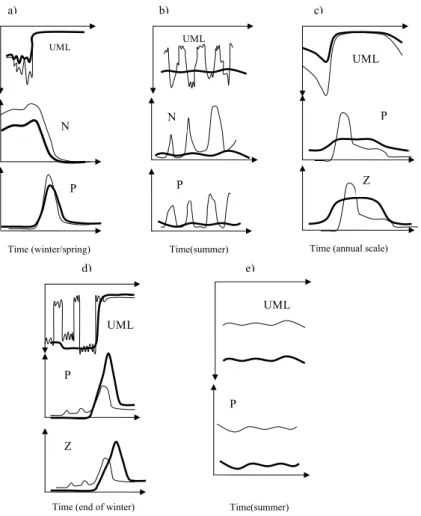
Fig. 1. Schematic representation of the main UML control mechanisms over ecosystem dynamics: (a) Impact of depth of winter mixing
(the major factor determining nutrient supply to the UML). Thick line describes a shallower (compared with the thin line) winter convection leading to lower nitrate concentration in the UML at the beginning of the spring, and a lower phytoplankton bloom terminated earlier by nutrient limitation. (b) Impact of short-term storm-induced summer deepening of the UML (enhances nutrient supply into the photic zone and primary production if it is nutrient-limited as opposed to light-limited). Thin line describes frequent deepenings of the UML as opposed to the stable depth (thick line) leading to the pulses of nutrients entrained from below the UML leading to an increase in phytoplankton biomass. (c) Impact of average winter mixing depth (influences the extent to which zooplankton can survive through the winter and hence exert grazing pressure on the spring phytoplankton bloom). The thin line describes a deeper (compared with the thick line) winter convection when primary production is low during the winter because of strong light limitation, leading to low zooplankton biomass which does not then put a significant grazing pressure on the spring phytoplankton bloom. In the case described by the thin line, zooplankton grazing suppresses the spring bloom. (d) Impact of short-term restratification of the UML during late winter and spring due to extremely calm weather followed by the return of deep mixing (such periods reduce light limitation and increase the level of coupling between phytoplankton and their grazers and change the dynamics of the spring bloom). Thin line describes a convective regime with a frequent near-surface restratification allowing significant production to occur, followed by the growth of zooplankton. At the moment of the spring bloom zooplankton population is then large enough to exert a significant grazing pressure on the phytoplankton. In the case of stable deep convection (thick line), the zooplankton population at the moment of the bloom is low and the first stage of the bloom develops without grazing pressure. (e) Impact of average summer mixed layer depth (determines light limitation of phytoplankton growth over the season). The thick line describes deeper (compared with the thin line) UML depth leading to higher light limitation of primary production and lower phytoplankton biomass.
3 Results
3.1 UML dynamics
The features of UML variability, on a range of timescales from diurnal to seasonal, which have the greatest influence on ecosystem dynamics through supply of nutrients, light
limitation and the impact of grazing are the following (pre-sented schematically in Fig. 1):
i) The maximum penetration of deep winter mixing (the major factor determining nutrient supply to the UML); ii) Frequency and maximum depth of short-term
0 50 100 150 200 250 300 350 400 −250 −200 −150 −100 −50 0 (a) KERFIX 0 50 100 150 200 250 300 350 400 −80 −60 −40 −20 0 (b) HOT 0 50 100 150 200 250 300 350 400 −100 −80 −60 −40 −20 0 (c) PAPA 0 50 100 150 200 250 300 350 400 1500 500 100 20 (d) INDIA 0 50 100 150 200 250 300 350 400 500 100 20 (e) BERMUDA Time (days)
Fig. 2. UML depth variability for the year 1992 at KERFIX (a),
HOT (b), Papa (c), India (d), BATS (e) in the control run (black dots), daily (red), weekly (green) and monthly (blue) forcing runs.
nutrient supply into the photic zone and primary produc-tion if it is nutrient-limited as opposed to light-limited); iii) Average winter mixing depth (influences the extent to which zooplankton can survive through the winter and hence exert grazing pressure on the spring phytoplank-ton bloom);
iv) Frequency and duration of short-term restratification of the UML during late winter and spring due to extremely calm weather followed by the return of deep mixing (such periods reduce light limitation and increase the level of coupling between phytoplankton and their graz-ers and change the dynamics of the spring bloom); v) Average summer mixed layer depth (determines light
limitation of phytoplankton growth over the season). In our analysis of the UML variability under the external forcing of the different frequencies, we focus on the particu-lar mechanisms described above. Note that the UML depth
0 10 20 30 40 −50 0 50
(a) Contr.Run.: min monthly UML
−5 0 5 10 15 20 0 100 200 300 −50 0 50 (b) Contr.R.: UMLmax−UMLmean
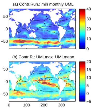
Fig. 3. (a) The monthly-averaged UML depth from the control run
for the month when it is at its minimum, in m. (b) Difference (in m) between the minimum monthly averaged daily maximum (night-time) UML depth and the minimum monthly-averaged UML depth. Black dots show the locations of the five time series stations dis-cussed in the text and shown on Figs. 2 and 10. Black line represents a mean annual nitrate concentration of 1 mmol m−3also shown in
Figs. 4, 7, 9, and chosen as a means of defining the boundaries be-tween different regions described in the text.
is defined here as the depth of the actively mixing layer. This may be deeper than the depth over which density is uniform – the mixed layer – during periods of active mixing, and con-siderably shallower than the mixed layer e.g. during the day-time where there is a strong diurnal cycle (see e.g. Brainerd and Gregg, 1996).
The annual cycle of UML depth as predicted by the model at five JGOFS locations (PC06) for monthly, weekly, daily and 6 h external forcing is shown in Fig. 2. The diurnal cycle of UML depth is resolved with 6 h forcing, showing a charac-teristic shallowing during the day and deepening during the night, a feature not captured with the other forcings.
The monthly-averaged UML depth from the control run is shown in Fig. 3a for the month when it is at its minimum. This minimum monthly UML depth is a convenient proxy for the summer-time average UML depth, and therefore the in-fluence of light limitation during the growing season (mech-anism v). It is independent of hemisphere, the existence of seasonal regimes such as monsoons, and the weak annual signal seen in equatorial areas. The deepest such minimum
UML depths are found over the Southern Ocean (∼40 m) and over the belts of strongest trade winds centred at 15◦N/S
(∼20 m).
The monthly averaged night-time UML depth gives a bet-ter idea of the depth of the mixed layer. It is deeper than the average UML depth by up to 20 m (Fig. 3b). These depths differ most over the trade wind belts of strong in-solation and strong winds (see also the seasonal cycle at HOT, Fig. 2b), and over the Antarctic Circumpolar Current (KERFIX, Fig. 2a), where, although insolation is weaker, the night-time UML is deepest so that any diurnal restratification reduces the mean UML depth significantly.
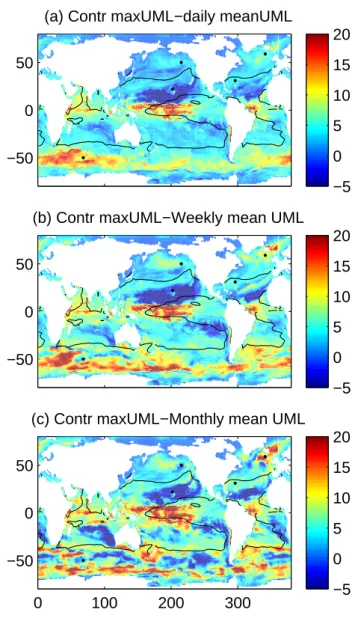
In the trade wind belts (see Fig. 4a–c and station HOT, Fig. 2b), the UML depth driven by the averaged forcings is similar to the night-time UML depths driven by the con-trol forcing. Here the wind is relatively steady, so the wind-energy available to drive mixing is not reduced much using the averaged forcings rather than the 6-hourly forcing. In the mid-latitudes and equatorial ocean, however, the variability of the wind on short timescales is significant relative to the mean winds. Hence there is more wind-energy in the con-trol run to drive mixing, and so the night-time concon-trol UML is deeper than that of the averaged runs (see station Papa – Fig. 2c, the North Pacific in Fig. 4a–c, INDIA – Fig. 2d, the North Atlantic in Fig. 4a–c).
At Bermuda (Fig. 2e) the extra summer mixing in the con-trol run is very marked. Here summer insolation is strong and the winds weak, and it seems that the mixed- layer model is unable to drive any significant mixing with averaged, even daily-averaged forcing. It may only permit mixing with weak winds where there are periods of buoyancy loss (i.e. by in-cluding the diurnal cycle).
When comparing the mean UML depth from the con-trol run against the UML depth from the averaged forcing runs (Fig. 5a–c), there are then two opposing effects. Since the daily mean UML is shallower than the night-time UML depth (see again Fig. 3b), the daily mean UML depth is shal-lower than the averaged forcing UML depths in regions like the trade wind belts (e.g. HOT, Fig. 2b) where the night-time UML depth was similar to the UML depths with av-eraged forcing. From a biological perspective, the similarity in night-time UML depth means that nutrient supply to the system remains unaltered (mechanisms i and ii). Limitation by light should however be significantly less in the 6 h run compared to the other forcings because of the shallowing of the UML during the day (mechanism v). But where the ex-tra wind energy of the 6 h dataset is more important in giv-ing deeper UMLs than this diurnal averaggiv-ing effect, the con-trol mean UMLs are deeper than the averaged forcing UMLs. This behaviour is seen at Papa, India and BATS (Fig. 2c, d, e). In these areas the 6 h forcing gives rise to the highest ver-tical flux of nutrients in the model, but is accompanied by the highest levels of light limitation.
The maximum penetration of deep winter mixing deter-mines a major part of the nutrient supply to the upper layer
−5 0 5 10 15 20 −50 0 50
(a) Contr maxUML−daily meanUML
−5 0 5 10 15 20 −50 0 50
(b) Contr maxUML−Weekly mean UML
−5 0 5 10 15 20 0 100 200 300 −50 0 50
(c) Contr maxUML−Monthly mean UML
Fig. 4. Difference (in m) between the minimum monthly averaged
daily maximum (night-time) UML depth in the control run and the minimum monthly-averaged UML depth in the runs driven by daily averaged (a), weekly averaged (b) and monthly averaged (c) forc-ing.
(mechanism i). It is plotted in Fig. 6a as the maximum monthly averaged daily maximum UML depth for the control run. This depth is largely set by accumulated buoyancy loss over the winter, and so is generally similar in the 6 h, daily and weekly runs. However the use of monthly forcing fields does substantially increase the maximum penetration of win-ter mixing in some areas (Fig. 2). The deviation of the max-imum over the year of the monthly-mean UML depth in the monthly run from that in the control run is shown in Fig. 6b. The northern boundaries of the northern subtropical gyres and areas of deep winter convection in the northern North Atlantic experience the largest difference. Winter mixing in
−1 −0.5 0 0.5 1 −50 0 50
(a) Control−Daily (UML min)
−1 −0.5 0 0.5 1 −50 0 50
(b) Control−Weekly (UML min)
−1 −0.5 0 0.5 1 0 100 200 300 −50 0 50
(c) Control−Monthly (UML min)
Fig. 5. Differences at each point between the minimum monthly
UML depth in the control run and in the runs driven by daily-averaged (a), weekly-daily-averaged (b) and monthly-daily-averaged (c) forc-ing, divided by the minimum monthly UML depth in the control run at that point. Differences in the following figures (except Fig. 6b) are also calculated in this way as XcontrolX−Xexperiment
control . Negative
val-ues highlight areas where averaging of the forcing fields leads pre-dicted summer-time UMLs being deeper than in the 6 h run. These areas include equatorward regions of the subtropical gyres, with sta-tion HOT being situated in one such area. Regions showing positive values which include the poleward parts of the subtropical gyres as well as moderate and high latitude areas of the Northern hemi-sphere, show shallower predicted UMLs when the forcing is aver-aged. Black dots show the locations of the five time series stations discussed in the text and shown on Figs. 2 and 10.
these areas when using monthly forcing is 3–4 times deeper than in the control run. The reasons for this are not entirely clear to us. We suppose that when weekly,daily or 6-hourly fields are employed, there are occasional periods of weak
0 100 200 300 −50 0 50
(a) Contr.R. UML max
−1 −0.5 0 0.5 1 0 100 200 300 −50 0 50
(b) Control−monthly (UML max)
Fig. 6. (a) The maximum monthly averaged daily maximum
(night-time) UML depth, in m. (b) The difference between the maximum monthly averaged daily maximum (night-time) UML depth (a) and the maximum monthly-averaged UML depth in the run driven by monthly-averaged forcing.
mixing. At these times eddy processes parameterized by the Gent and McWilliams bolus transport may operate so as to restratify the “fossil” mixed layers left behind. This addi-tional stratification is suppressed if monthly averaged fields are employed, as the Gent and McWilliams process is not active within the mixed layer itself. Station India, which is located on the periphery of one such area, shows a doubling of the maximum depth of winter mixing under the monthly forcing (Fig. 2d, note the logarithmic scale). The impact of using monthly forcing fields on the maximum depth of the winter mixing does not exceed 20% in the rest of the ocean, and so is only of relatively minor significance for ecosystem dynamics.
UML variability during the winter is substantially different under the different external forcings (mechanism ii). UML in the 6 h run exhibits frequent periods of near surface restrati-fication followed by the return of winter convection (Fig. 2). Daily average forcing produces a relative constancy in the depth of the UML, with no periods of restratification be-tween the storms in moderate and high latitudes (e.g. India, KERFIX, Papa, Fig. 2). In low latitudes, however, daily av-eraged forcing does resolve periods of shallow stratification (see HOT and BATS, Fig. 2). In the weekly and monthly runs, these periods are absent even at low latitudes.
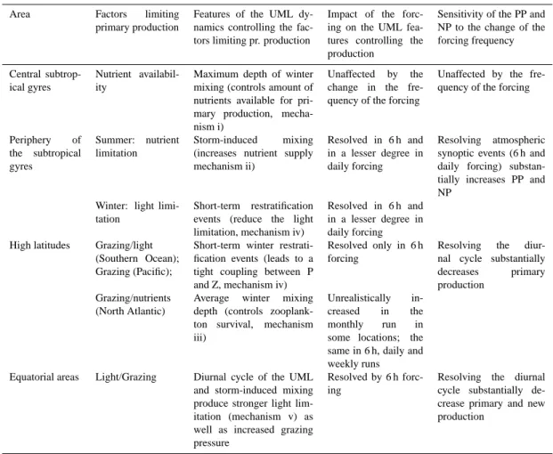
Table 1. Impact of the variation of the external forcing frequency on the primary production in the subtropical gyres, high and moderate
latitudes and equatorial region.
Area Factors limiting
primary production
Features of the UML dy-namics controlling the fac-tors limiting pr. production
Impact of the forc-ing on the UML fea-tures controlling the production
Sensitivity of the PP and NP to the change of the forcing frequency
Central subtrop-ical gyres
Nutrient availabil-ity
Maximum depth of winter mixing (controls amount of nutrients available for pri-mary production, mecha-nism i)
Unaffected by the change in the fre-quency of the forcing
Unaffected by the fre-quency of the forcing
Periphery of the subtropical gyres Summer: nutrient limitation Storm-induced mixing
(increases nutrient supply mechanism ii)
Resolved in 6 h and in a lesser degree in daily forcing
Resolving atmospheric synoptic events (6 h and daily forcing) substan-tially increases PP and NP
Winter: light limi-tation
Short-term restratification events (reduce the light limitation, mechanism iv)
Resolved in 6 h and in a lesser degree in daily forcing High latitudes Grazing/light
(Southern Ocean); Grazing (Pacific);
Short-term winter restrati-fication events (leads to a tight coupling between P and Z, mechanism iv)
Resolved only in 6 h forcing
Resolving the diur-nal cycle substantially
decreases primary
production Grazing/nutrients
(North Atlantic)
Average winter mixing
depth (controls zooplank-ton survival, mechanism iii)
Unrealistically
in-creased in the
monthly run in
some locations; the same in 6 h, daily and weekly runs Equatorial areas Light/Grazing Diurnal cycle of the UML
and storm-induced mixing produce stronger light lim-itation (mechanism v) as well as increased grazing pressure
Resolved by 6 h forc-ing
Resolving the diurnal cycle substantially de-crease primary and new production
3.2 Primary and new production
In this section we examine the impact of the frequency of external forcing, as manifested in UML variability, on pri-mary and new production. The impacts of the different forc-ings vary markedly between oligotrophic areas of the sub-tropical gyres, high and moderate latitudes, and equatorial areas (Fig. 7, Table 1). A mean annual nitrate concentration of 1 mmol m−3, as shown in Figs. 5, 4, 7, 9, was chosen as
a means of defining the boundaries between these different regions. The resulting mean annual integrated primary and new production for these areas is shown in Fig. 8. Analysis was restricted to areas free from seasonal ice cover (between 60◦S and 70◦N) since the variation of the ice boundary with
that of the external forcing frequency is significant and be-yond the scope of this paper. The primary production at five JGOFS locations for each of the model runs is presented in Fig. 10. As shown in Fig. 8, the major change in the global primary and new productions occurs when the frequency of the external forcing increases from daily to 6 h. In this case global (excluding zones affected by the seasonal ice cover)
primary production declines by about 25% while the new production declines by about 10%. Equatorial and high lat-itude areas contribute most toward the decrease, while olig-otrophic gyres show a small increase in both new and total primary production. Decreasing the forcing frequency from daily to weekly and then monthly impacts on the production to a much lesser degree with the effect not exceeding 5–7%. Regional variations can however be quite high (see the dis-cussion below).
3.2.1 High and moderate latitudes
The area of high and moderate latitudes includes three sub-stantially different sub-areas within the model: the subarctic Pacific, northern North Atlantic and the Southern Ocean. The subarctic Pacific is characterised by relatively shallow win-ter mixing compared with that of the same latitudes of the North Atlantic and Southern Ocean. This lack of deep win-ter convection allows the modelled zooplankton populations to survive in numbers throughout the winter and exert sig-nificant grazing control over the primary production. Station
−1 −0.5 0 0.5 1 −50 0 50 a) Control−Daily (pr.prod) −1 −0.5 0 0.5 1 −50 0 50 b) Control−Weekly (pr. prod) −1 −0.5 0 0.5 1 0 100 200 300 −50 0 50 c) Control−Monthly (pr. prod) −1 −0.5 0 0.5 1 −50 0 50
d) Control−Daily (new prod)
−1 −0.5 0 0.5 1 −50 0 50
e) Control−Weekly (new prod)
−1 −0.5 0 0.5 1 0 100 200 300 −50 0 50
f) Control−Monthly (new prod)
Higher than control run
Fig. 7. Deviation of the mean annual primary production in the control run (see Fig. 5 for additional explanation) from the daily forcing run (a), weekly forcing run (b), monthly forcing run (c); deviation of the mean annual new production in the control run from the daily forcing
run (d), weekly forcing run (e), monthly forcing run (f). Black dots show the locations of the five time series stations discussed in the text and shown on Figs. 2 and 10.
Olig Equat H.lat Total 0 10 20 30 40 50
Primary production (GtC/yr)
Olig Equat H.lat Total 0 2 4 6 8 10
New production (GtC/yr)
Fig. 8. Mean annual primary (a) and new (b) production (GtC yr−1)
integrated over the equatorial, oligotrophic and high latitude areas (see text) and the global ocean for the 6 h (dark blue), daily (light blue), weekly (yellow) and monthly (red) forcing runs.
Papa (Figs. 2c, 10c) provides a good example of ecosystem dynamics in the subarctic Pacific (PC06).
In contrast, the high and moderate latitudes of the North Atlantic exhibit a pronounced spring bloom initiated by sta-ble stratification after deep winter convection. At the high-est latitudes this bloom is predicted to subside before nutri-ents are depleted, a result of top-down control by zooplank-ton grazers. Station India (PC06) is typical of this domain (Figs. 2d, 10d). Further south, the bloom is terminated after nutrient exhaustion, its magnitude depending on the depth of the preceding winter convection. Predicted ecosystem dy-namics at Bermuda (Figs. 2e, 10e), which is situated on the periphery of the oligotrophic gyre, show features of both the oligotrophic and moderate latitude regimes due to its rela-tively deep (200–350 m) winter convection.
Primary production in the Southern Ocean is limited in the model by both grazing and light. In a similar fashion to the high latitudes of the Pacific Ocean, this area does not expe-rience deep winter convection, a situation leading to grazing control over phytoplankton growth in spring. Light limita-tion of primary produclimita-tion is also prevalent in summer due to the extremely deep UML that occurs at that time of year (PC06). Station Kerfix (PC06) provides a good example of ecosystem dynamics in the Southern Ocean (Figs. 2a, 10a).
Lowest rates of new and total primary production were predicted when using the 6 h external forcing in these ar-eas (Figs. 7, 8). Using the higher frequency external forcing reduces the predicted magnitude of the spring bloom in the North Atlantic, while in the Pacific and Southern ocean the primary production is reduced throughout the whole sum-mer period. The cause of this reduction is related to short-term spring restratification events (mechanism iv) which oc-cur when the system oscillates between deep winter convec-tion and a shallow stable UML. During such periods, both the phytoplankton and zooplankton populations develop quickly together such that when conditions are ideal for phytoplank-ton to bloom, the zooplankphytoplank-ton population is sufficiently large to exert top-down control and thereby prevent any bloom from occurring. Such periods do not occur when using the monthly and weekly forcings, while in the daily run they are much less frequent than in the run with the 6 h external forc-ing.
In order to examine the strength of grazing in controlling primary production (mechanisms iii and iv) we chose as a proxy the surface mean annual zooplankton to phytoplankton ratio (Fig. 9). This ratio illustrates the significant increase in grazing pressure at high latitudes that is predicted when the diurnal cycle is resolved (Fig. 9a), most significantly in the subarctic Pacific, and to a lesser degree in the Southern Ocean and the northern North Atlantic. While the largest changes are obtained by resolving the diurnal cycle, the dif-ference between the production predicted under daily and weekly forcings is negligible. The depth of winter convec-tion remains the same when the forcing frequency decreases from 6 h to weekly, thus rendering mechanism (iii), the effect of grazing pressure, inactive. However, the use of monthly forcing significantly deepens the predicted winter convection in the northern North Atlantic (Fig. 2d, India, and 2e, BATS, see also Fig. 6b) and leads to much larger blooms than in any of the other runs, the reduction in grazing pressure once again being of importance. The importance of resolving the diur-nal cycle suggests that mechanism iv (short-term spring re-stratification) plays the dominant role in controlling primary production and that it is necessary to resolve the diurnal cy-cle if the coupling between phytoplankton and zooplankton is to be modelled adequately.
The use of 6 h forcing, and its impact on the coupling be-tween phytoplankton and zooplankton, has a much greater effect on total primary production than on the new produc-tion (cf. Figs 7a–c and 7d–f). Resolving the diurnal cycle in
−0.2 −0.1 0 0.1 0.2 −50 0 50 a) Control−Daily (Z/P) −0.2 −0.1 0 0.1 0.2 −50 0 50 b) Control−Weekly (Z/P) −0.2 −0.1 0 0.1 0.2 0 100 200 300 −50 0 50 c) Control−Monthly (Z/P) Higher than control run
Fig. 9. Deviation of the surface phyto- to zooplankton ratio in the
control run (see Fig. 5 for additional explanation) from the daily forcing run (a), weekly forcing run (b), monthly forcing run (c). Black dots show the locations of the five time series stations dis-cussed in the text and shown on Figs. 2 and 10.
the Southern Ocean, for example, reduces primary produc-tion by 30–40% while new producproduc-tion remains almost unaf-fected. This difference is because the zooplankton grazing pressure affects the amount regenerated rather than new pro-duction.
3.2.2 Subtropical gyres
Deep winter mixing is absent in the central areas of the sub-tropical oligotrophic gyres and so primary production is lim-ited primarily by nutrient availability. Station HOT provides a good example of ecosystem dynamics in the oligotrophic gyres (PC06). The absolute maximum depth of the UML
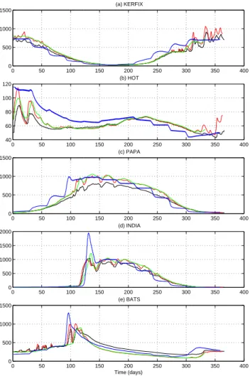
0 50 100 150 200 250 300 350 400 0 500 1000 1500 (a) KERFIX 0 50 100 150 200 250 300 350 400 40 60 80 100 120 (b) HOT 0 50 100 150 200 250 300 350 400 0 500 1000 1500 (c) PAPA 0 50 100 150 200 250 300 350 400 0 500 1000 1500 2000 (d) INDIA 0 50 100 150 200 250 300 350 400 0 500 1000 1500 (e) BATS Time (days)
Fig. 10. Photic zone integrated primary production (mgC m−2d−1)
for the year 1992 at KERFIX (a), HOT (b), Papa (c), India (d), BATS (e) in the control run (black), daily (red), weekly (green) and monthly (blue) forcing runs.
is the factor determining the nutrient supply (mechanism i) in these areas and hence also annual primary and new pro-duction. As was shown above, this depth is the same in the 6 h, daily and weekly run (Fig. 2b, station HOT), and so the predicted annual primary and new production remain almost unaffected by the change in the frequency of the forcing.
On an intra-annual time scale, winter productivity peaks in the 6 h run are lower than in the daily forcing run (Fig. 10b). These peaks occur during periods of calm weather between storms, which are generally persistent for a few days in the daily forcing run, while being interrupted by the deeper night-time UML in the 6 h run (Fig. 2b). Since the nutrient supply from below is the same in 6 h and daily runs (mech-anism ii), resolving the diurnal cycle reduces the amplitude of blooms of phytoplankton because of the stronger impact of light limitation (mechanism v). In the weekly run, winter restratification periods are almost absent. The system
dur-ing the winter is shifted towards light limitation more than in 6 h and daily runs and the magnitude of the winter blooms is somewhat different. This effect is not however system-atic and does not affect annual ecosystem characteristics con-trolled by the depth of maximum winter mixing. Primary production in the monthly run shows the single winter maxi-mum and summer minimaxi-mum without any smaller-scale oscil-lations.
Towards the periphery of the gyres, where winter mixing can reach significant depths, primary production is limited by nutrient availability only in summer. Light conditions play the dominant role in winter, although primary produc-tion during this season remains high. In these areas, an in-crease in frequency of the external forcing inin-creases both pri-mary and new production by up to a factor of two (Fig. 7). Two mechanisms are responsible for this enhanced produc-tivity. The first involves the existence of short-term periods of shallow stratification during calm weather in winter. Dur-ing such periods, which last from one to two days and are well resolved in the 6 h and daily runs, light conditions are ameliorated and significant production occurs. The effect is usually more pronounced in the daily run because such shal-lowings are not predicted to be interrupted by deepening of the mixed layer during the night. UML dynamics of this type are seen in the model at BATS (Figs. 2e and 10e), although responses to forcings at this station are more typical of those of the moderate latitudes, as is discussed below. The second mechanism involves the prediction of deeper storm-induced mixing in summer in the 6 h run (Figs. 2e and 10e), which increases the nutrient supply and therefore tends to increase productivity. Unlike in the centres of the gyres, predicted nutrient concentrations below the UML in summer are still significant. Nutrient supply from below is then enhanced by night-time deepenings and better resolved storm-induced mixing in the 6 h run.
The two mechanisms described above do not however ap-ply to the monthly forcing which generates unrealistically deep mixing over some areas of the gyres, especially in the northern hemisphere, where winter mixing can deepen by a factor of 3–4 (Fig. 6b). Such a deepening significantly in-creases nutrient supply to the gyre and doubles primary pro-duction in the areas where limitation by nutrients substan-tially exceeds that by light (Fig. 7c, f). On the other hand, production in the areas which are more severely limited by light, such as southern parts of the southern gyres, declines by a factor of two, so that total production in the subtropical gyres remains the same (Fig. 8).
3.2.3 Areas affected by equatorial and coastal upwelling In the equatorial areas, monthly, weekly and daily averaged forcing produce very similar results. Resolution of the diur-nal cycle did however decrease predicted primary production by about 30–50% (Fig. 7) by increasing the averaged UML depth (mechanism v), impacting on the light limitation of
phytoplankton growth (Fig. 5a–c) and also increasing graz-ing pressure (Fig. 9a). The impact of the 6 h forcgraz-ing on new production is much smaller and does not exceed 20%. This effect is minimal because equatorial upwelling, the main source of new nutrients in the area, remains mostly unaf-fected by variations in wind frequency.
The total predicted new and primary production of the equatorial area in the 6 h run is considerable, being around 2 and 10 Gt C yr−1for each area respectively (Fig. 8). These
values increase to 2.3 and 15 Gt C yr−1in the run with daily
average forcings. The significance of these changes are not just local, but extend to have a major impact on the global predictions of primary and new production.
4 Discussion
The sensitivity of ecosystem dynamics to the high frequency variations in external forcing, with resulting consequences for variability in the UML, was investigated using a global ecosystem model. The motivation for the work was the fact that global or basin-scale models often use simplistic repre-sentations of the UML and/or low frequency external forc-ing and are therefore unable to capture short-term variabil-ity in the UML. The model of Aumont et al. (2003), for example, has no explicit treatment of the UML, using in-stead a photic zone of 100 m that undergoes vertical mix-ing with neighbourmix-ing 50 m deep grid cells. Likewise, the use of long time steps, a common feature of global models subjected to lengthy runs, ignores short term variations in UML. The model of Six and Maier-Reimer (1996), for ex-ample, uses a time step of one month. In similar fashion, the bulk Krauss-Turner mixed layer scheme employed by Palmer and Totterdell (2001) employs monthly mean external forc-ing, with further difficulties arising from the homogenising of state variables throughout even the deepest UMLs.
In our study we compared four runs of a global GCM driven by monthly, weekly, daily and 6 h external forcing. Results showed that resolving diurnal variation in forcing had impacts on predicted global patterns of primary and new production extending far beyond this timescale. Globally integrated values of primary and new production were sig-nificantly altered when using high frequency forcing. An intriguing discovery was that episodic events of very calm, rather than very stormy, weather had the greatest impact on predicted primary production, and that furthermore the events during the winter months were of greatest signifi-cance.
It should be emphasised that the difference between the daily and 6 h external forcing is not only in resolving the di-urnal cycle of the forcing and consequently of the UML with deepening during the night and shallowing during the day. In addition, the 6 h forcing provides a much improved res-olution of extreme values of the wind stress during storms as well as a better representation of occasional very calm
weather, both of which are usually persistent for a day or two. The time scale of these events is too short to be prop-erly resolved by using daily averaged forcing.
To what extent, then, were predicted new and total primary production improved when using 6 h forcing? One problem area for modellers has always been the oligotrophic gyres in which primary production tends to be severely underesti-mated in both global and basin-scale models (e.g. Sarmiento et al., 1993; Oschlies et al., 2000). Although predicted pri-mary production in the centre of the oligotrophic gyres was unaffected by the increase in the frequency of the external forcing, and still lower than observed, the peripheries of the gyres showed a significant increase in productivity locally reaching a factor of two when the diurnal cycle was resolved. Two mechanisms are responsible for this increase. The first, affecting mostly regenerated production, is associated with short-term periods of shallow stable stratification during the winter when significant production can occur due to reduced limitation by light. The second mechanism, mostly affect-ing new production, is associated with storm-induced mixaffect-ing during spring and summer, which increases vertical nutrient supply. In order to adequately describe the impact of these mechanisms on primary production, a model of atmospheric forcing should resolve not only synoptic atmospheric events but also the diurnal cycle of the forcing fields resulting in the diurnal UML variability which enhances the effect of both of the above mentioned mechanisms.
Another problem area for GCM modellers has been over-estimation of primary production in equatorial areas (Os-chlies et al., 2000). Results here show that high frequency external forcing may significantly improve the performance of global models in these areas, providing a much deeper predicted UML, and at least partly overcome the problem of overestimated primary production. This overestimation is usually attributed to overestimation in the intensity of up-welling (Oschlies et al., 2000). In fact, the band of high pro-duction at the equator can be subdivided into two areas char-acterised by different physical regimes, but leading to similar ecosystem responses (PC06). One is the equatorial upwelling area with a shallow stable UML, which is surrounded by a second area of equatorial currents with a deeper UML than in the adjacent oligotrophic gyres. This second area therefore has a greater potential for light limitation to suppress primary production. It is therefore important to resolve the significant storm activity in this area, as well as the diurnal cycle of the UML layer, both of which contribute towards stronger light limitation of primary production. Resolving the diurnal cycle by using the 6 h external forcing caused a decrease of 30% in predicted primary production of the total equatorial area, the effect being locally as much as factor of five.
In the high-nutrient low-chlorophyll Southern Ocean and subarctic Pacific, the use of 6 h forcing gives rise to rela-tively tight coupling between phytoplankton and herbivorous zooplankton. The result is relatively low primary production and low seasonality of the Chl-a, showing better agreement
with data compared to the runs using other forcings. Short bursts of relatively calm weather during the winter create mini-blooms of phytoplankton and zooplankton in these ar-eas. These bursts serve to sustain the zooplankton popu-lation in the model, which is then sufficiently well devel-oped to suppress the development of phytoplankton blooms, the grazing control of productivity extending into the sum-mer. Increasing the frequency of external forcing from 6 h to 24 h led to a decline in predicted global primary production (excluding areas affected by seasonal ice cover) from 41 to 33 Gt C yr−1. The impact of this increase in forcing period on
new production is however much smaller being 0.5 Gt C yr−1
which is only about 10% of the total annual value. This effect is relatively small because most of the mechanisms that are sensitive to high frequency forcing affect zooplankton graz-ing pressure which impacts mainly on regenerated rather than new production.
In spite of the generally good agreement with observa-tions, our model has significant limitations with respect to both the ocean dynamics and ecosystem structure. The 1◦
resolution means that shelf areas are not represented, and ar-eas affected by sar-easonal ice cover are only poorly resolved. Mesoscale motion, with its tendency to enhance the horizon-tal and vertical transports of nutrients, is nonexistent in the model. We can speculate that an increase in resolution will give further improvement in the model performance in the centre of the oligotrophic gyres where the primary produc-tion still remains underestimated. The increase of the nutri-ent supply on the peripheries of the gyres achieved by the higher forcing frequencies can lead to significant intensifica-tion of the lateral eddy transport of nutrients towards the cen-tre of the gyres in eddy-resolving models. This point serves only to strengthen the rationale for the need to pay attention to realistically formulating physics in GCMs if reliable pre-dictions of biophysical interactions are to be made.
The introduction of additional factors limiting primary production was needed in order to better describe region-ally important factors such as micronutrient limitation in the Southern Ocean and nitrogen fixation in the oligotrophic gyres. Nevertheless, in spite of the effect of these short-comings on the analysis above, the impact of high frequency forcing on the mechanisms influencing primary production (Fig. 1) has been unequivocally demonstrated. Much of the current emphasis on future directions in global biogeo-chemical modelling is directed towards increasing complex-ity in the ecosystems models used (e.g. LeQuere, 2005), al-though it is by no means clear whether the resulting param-eterizations are sufficiently robust to perform in, for exam-ple, climate predictions (Anderson, 2005). The results pre-sented here demonstrate the importance of increasing phys-ical complexity in order for numerphys-ical models to accurately capture climate change impacts and subsequent biotic feed-backs. Accurate representation of physical processes is nec-essary before one can hope to achieve realism in predicted biogeochemical fields and their response to climatic forcing.
Of course the biological parameterizations are important too. For example, our results show that the grazing control of primary production is sensitive to variations in the external forcing. Physics and biology alike require consideration if biophysical interactions are to be realistically captured when modelling biogeochemistry in GCMs.
5 Conclusions
The use of 6 h, daily, weekly and monthly forcing of atmo-spheric fields resulted in dramatically different predictions of plankton productivity in a global 3-D coupled physical-biogeochemical model. Resolving the diurnal cycle of at-mospheric variability using of 6 h forcing, and hence also diurnal variability in UML depth, produced the largest dif-ference, reducing predicted global primary and new produc-tion by 25% and 10% respectively relative to that predicted with lower frequency forcing. This variation varied region-ally, being a 30% reduction in equatorial areas, 25% at mod-erate and high latitudes and a 10% increase in the periph-eries of the oligotrophic gyres. Predicted primary and new production in the centres of the oligotrophic gyres remains unaffected by the frequency of the external forcing because the maximum depth of the UML throughout the year was in-dependent of the frequency of forcing and the depth of the nitracline is deeper than the maximum UML depth. In these areas, severely limited by nutrient availability, this depth is the main factor determining mean annual primary and new production.
Two mechanisms associated with short term episodic mix-ing are of greatest importance in contributmix-ing to the differ-ences in primary production predicted for different forcings. The first is restratification events during periods of calm weather between storms in winter, which are well resolved under the 6 h forcing. The use of daily forcing also resolved these events, but to a lesser degree. Significant growth of phytoplankton occurs during these periods of restratification, thus enhancing the predicted annual production. Moreover, these events tend to enhance coupling between phytoplank-ton and their herbivorous grazers, preventing the occurrence of blooms at high latitudes and thus reducing annual primary and new production in these areas. Second, the use of 6 h forcing permits a good resolution of maximum wind speed during storm events, thus generating deeper mixing than in runs with lower frequency forcing.
Resolution of the diurnal cycle of the UML, with its deep-ening during the night and shallowing during the day, also affects averaged UML depth and so significantly influences productivity. It is the UML depth averaged over the sum-mer period that determines the level of ligh limitation of an-nual primary production. Average winter mixing depth influ-ences the extent to which zooplankton can survive through the winter and hence exert grazing pressure on the spring phytoplankton bloom. The use of monthly forcing gave rise
to various unrealistic features in both the physical and bi-ological variables of the model. Unrealistically deep win-ter convection was predicted in the moderate latitudes of the North Atlantic and North Pacific oceans, causing a dramatic increase in predicted primary and new production. In addi-tion, model runs employing either monthly or weekly forcing fields are missing important mechanisms that control primary and new production, namely episodic storm-induced mixing and short-term winter time near-surface restratification dur-ing the calm weather, and cannot therefore be recommended for use in predicting, for example, the response of the ma-rine biota to climate change. Although daily forcing gives a relatively good description of some mechanisms involved in controlling primary production such as the impact of storms, it smoothes out the diurnal cycle of the UML which has a profound implications regarding the light limitation of the productivity. Thus resolving the diurnal cycle in the equa-torial areas reduced primary production by 30% due to the increase of limitation by light.
By resolving the diurnal cycle in a 3-D coupled physi-cal and biologiphysi-cal model, performance was significantly im-proved with respect to several common problems: underesti-mated primary production in the oligotrophic gyres; overes-timated primary production in the Southern Ocean; overesti-mated magnitude of the spring bloom in the subarctic Pacific Ocean, and overestimated primary production in equatorial areas. The result of using 6 h forcing on predicted ecosystem dynamics was profound, the effects persisting far beyond the hourly timescale, and having major consequences for pre-dicted global and new production on an annual basis. Acknowledgements. The work had been supported by the Natural
Environment Research Council core strategic programs BICEP (Biophysical Interactions and Controls on Export Production) and LSTOC (Large Scale Long Term Ocean Circulation).
Edited by: V. Garcon
References
Anderson, T. R.: Plankton functional type modelling: running be-fore we can walk?, J. Plankton Research, 27, 1073–1081, 2005. Aumont, O., Maier-Reimer, E., Blain, S., and Monfray, P.:
An ecosystem model of the global ocean including Fe, Si, P colimitations, Global Biogeochem. Cy., 17, 29.1–29.15, doi:10.1029/2001GB001745, 2003.
Brainerd, K. E. and Gregg, M. C. : Surface mixed and mixing layer depths, Deep-Sea Research, 42, 1521–1543, 1996.
Conte, M. H., Dickey, T. D., Weber, J. C., Johnson, R. J., and Knap, A. H.: Transient physical forcing of pulsed export of bioreactive organic material to the deep Sargasso Sea, Deep Sea Research I, 50, 1157–1187, 2003.
Dickey, T., Zedler, S., Frye, D., Jannasch, H., Manov, D., Sigurd-son, D., McNeil, J. D., Dobeck, L., Yu, X., Gilbo, T. Y., Bravo, C., Doney, S. C., Siegel, D. A., and Nelson, N.: Physical and biogeochemical variability from hours to years at the Bermuda
Testbed Mooring: June 1994–March 1998, Deep Sea Research, II, 48, 2105–2140, 2001.
Fasham, M. J. R., Ducklow, H. W., and McKelvie, S. M.: A nitrogen-based model of plankton dynamics in the oceanic mixed layer, J. Mar. Res., 48, 591–639, 1990.
Fasham, M. J. R. and Evans, G. T.: The use of optimisation tech-niques to model marine ecosystem dynamics at the JGOFS sta-tion at 47◦N 20◦W, Phil. Trans. Roy. Soc. Lond., B 348, 206–
209, 1995.
Follows, M. and Dutkiewicz, S.: Meteorological modulation of the North Atlantic spring bloom, Deep Sea Res., Part II, 49, 321– 344, 2002.
Karl, D. M., Dore, D. E., Lucas R., Michaels, A. F., Bates, N. R., and Knap, A.: Building the long-term picture: the US JGOFS time-series Programs, Oceanogr., 14, 6–17, 2001.
Kawamiya, M. and Oschlies, A.: Simulated impact of intraseasonal variations in surface heat and momentum fluxes on the pelagic ecosystem of the Arabian Sea, J. Geophys. Res., 109, C03016, doi:10.1029/2003JC002107, 2004.
Large, W. G., Danabasoglu, G., and Doney, S. C.: Sensitivity to Surface Forcing and Boundary Layer Mixing in a Global Ocean Model: Annual-Mean Climatology, J. Phys. Oceanogr., 27, 2418–2446, 1997.
LeQuere, C., Harrison, S. P., Prentice, I. C., et al.: Ecosystem dy-namics based on plankton functional types for global ocean bio-geochemistry models, Global Change Biology, 11, 2016–2040, 2005.
McCreary, J. P., Kohler, K. E., Hood, R. R., Smith, S., Kindle, J., Fischer, A., and Weller, R. A.: Influences of diurnal and intrasea-sonal forcing on mixed-layer and biological variability in the central Arabian Sea, J. Geophys. Res., 106, 7139–7155, 2001. Oschlies, A.: Equatorial nutrient trapping in biogeochemical ocean
models, the role of advection numerics, Global Biogeochem. Cy-cles, 14, 655–667, 2000.
Oschlies, A., Koeve, W., and Garc¸on, V.: An eddy-permitting cou-pled physical-biological model of the North Atlantic 2. Ecosys-tem dynamics and comparison with satellite and JGOFS local studies data, Global Biogeochem. Cy., 14, 499–523, 2000. Palmer, J. R. and Totterdell, I. J.: Production and export in a global
ecosystem model, Deep-Sea Research I, 48, 1169–1198, 2001. Popova, E. E., Coward, A. C., Nurser, G. A., DeCuevas, B., and
Anderson, T. R.: Mechanisms controlling primary and new pro-duction in a global ecosystem model – Part I: Validation of the biological simulation, Ocean Sci., 2, 249–266, 2006,
http://www.ocean-sci.net/2/249/2006/.
Sarmiento, J. L., Slater, R. D., Fasham, M. J. R., Ducklow, H. W., Toggweiler, J. R., and Evans, G. T.: A seasonal three-dimensional ecosystem model of nitrogen cycling in the North Atlantic euphotic zone, Global Biogeochem. Cycles, 7, 417–450, 1993.
Six, K. D. and Maier-Reimer, E.: Effects of plankton dynamics on seasonal carbon fluxes in an ocean general circulation model, Global Biogeochem. Cy., 10, 559–583, 1996.
Waniek, J.: The role of physical forcing in initiation of spring blooms in the Northeast Atlantic, J. Mar. Syst., 39, 57–82, 2003.