SEISMIC MEASUREMENTS
byChengbin Peng, C.H. Cheng, and M.N. Toksoz Earth Resources Laboratory
Department of Earth, Atmospheric, and Planetary Sciences Massachusetts Institute of Technology
Cambridge, MA 02139
ABSTRACT
An exact formulation for borehole coupling, which is valid for all frequencies and all azimuthally symmetric and nonsymrnetric components, is given in this paper. The bore-hole effects on downbore-hole measurements are studied in detail as functions of frequency, incidence angle and polarization of an incident wave as well as geophone orientation. We found that correction of the borehole effect for downhole measurements should be made for frequencies above 500 Hz in a hard formation. In a soft formation, if the incidence angle is well away from the resonance angle for a SV incidence, no borehole correction is needed for frequencies below 300 Hz; while for frequencies above 300 Hz, the borehole can cause severe problems on downhole measurements. The borehole can also significantly alter the particle motion direction such that horizontal components rotation from data itself is unreliable for experiments with frequencies above 1 kHz in the hard formation and around 500 Hz in the soft formation.
INTRODUCTION
Increasing interest is shown towards the crosshole and VSP surveys at frequencies up to 1 kHz or more in order to resolve the fine details of structures and lithology between wells (Bregman et al, 1989; HarriS, 1988; Tura, 1991). However, at frequencies on the order of 1 kHz, the existence of a fluid-filled borehole has strong influence on the downhole measurements. Dependent on the frequency and angle of incidence, as well as the formation properties, the measured displacement on the borehole wall or pressure at the center of the fluid may be significantly different from that of the incident wave. Without proper attention to this effect, imaging and inversion techniques that utilize both the amplitude and phase information of recorded energy may be erroneous because the borehole is not included as part of the formulation.
(1) White (1953) presented a picture of the borehole coupling at zero frequency limit. As frequency goes to zero, the size of the borehole becomes much smaller than the wavelength such that the stress caused by an incident elastic plane wave is almost ho-mogeneous at the vicinity (much larger than the borehole radius) around the borehole if the borehole does not exist. Introduction of a borehole will locally disturb the homo-geneous stress field and the change of shape of the borehole can be exactly computed (Timoshenko and Goodier, 1951). The volume change of the borehole sets up a pressure inside the fluid in the same way as a piston source does. Schoenberg (1986) developed a complete theory for the interaction of a plane elastic wave with a fluid-filled borehole and gave an explicit formuiation for the low-frequency limit. In this theory the elastic field in the solid and the acoustic field inside the fluid satisfy the corresponding wave equations and coupling of these two fields is accomplished through the fluid-solid inter-face boundary conditions. Lovell and Hornby (1990) presented a complete formuiation for both low and high frequency for the azimuthally symmetric component, so their formulation can oniy apply to the pressure measurement at the center of the borehole. They found that for certain angles and for high enough frequencies (10 kHz) marked resonances in the fluid occur for both shear and compressional incidence.
In this paper, an exact formuiation based on Schoenberg's theory is given for all frequencies and all azimuthally symmetric and nonsymmetric components. Detailed studies on the influence of frequency, incidence angle and polarization of incoming elastic waves (P, SV and SH), as well as the geophone orientation, on the downhole measurements are given, both for the hard formation (exampled by Berea Sandstone) and the soft formation (exampled by Pierre Shale).
THEORETICAL FORMULATION
Consider an elastic wave incident on an infinite borehole drilled through a homogeneous elastic medium with density p, compressional wave speed Ct and shear wave speed {3. The borehole is filled with fluid which has density Pf and compressional wave speed Ctf. The radius of the borehole is Tb. When the wave hits the borehole, a transmitted compressional wave (denoted by displacement fj/) is generated in the fluid, and at the same time a scattered elastic wave (denoted byUS) is produced in the solid. Ifa three component geophone is placed in the fluid,
u
f will be recorded and if it is clamped against the formation, iJ}+
US will be measured, where iJ} denotes the incident wave.The fluid displacement
u
f can be expressed in terms of a potential1/J
f which satisfiesthe fluid wave equation as
w
2\l21/Jf
+
21/J
f=
0,
Ctf
represented by three elastic potentials </> (P potential), ~ (SV potential) and
'I/J
(SH potential) as (2) where 2 \72</>+
w2</>= 0 a w2 \72~+
{32~= 0 w2 \72'I/J+
{32'I/J=
o.
The general solution of these potentials is given by Schoenberg (1986) as
</>f =
a(;~w)
[AoJo(kfr)+2
L~=lin(Ancosne
+
A~sinne)Jn(kfr)]
</> _ - a~\,"J) [BoHg1)(kpr)
+
2L~=lin(Bncosne+
B~sin ne)H,\l) (kpr)J~
i{32;JW) [CoHa1)(ksr)+2L~=lin(Cncosne+C~sinne)H,\1)(ksr)]
'I/J
=_{3~SW) [-D~Hal)(ksr) +2 L~=lin(Dnsinne
-D~cosne)H,\l)(ksr)]
(3) wherez
dependence and time dependenceei(kzz-wt) is assumed, andk f=
V
w2 /a} - kz2, kp = vw2/a2 -kz2and ks =VW
2/{32_kz2. Signs of kf, kp, kz are chosen such that Im(kp, k., k f )~o.
Given these potentials in (3), the displacement and stress components that are involved in the boundary conditions can be written as
a(;~w)
[U!o(r)Ao+
2L~=linU!n(r)(Ancosne
+
A~sin
nell -a~sw)
[U!o(r)Bo+
2L~=linutn(r)(Bncosne
+
B~sin
nell_{3~SW)
[U;o(r)Co+
2L~=linU$n(r)(Cncosne
+
C~sinne)]
-
§~\,"')
[U:{;(r)Do+
2L~=linU%(r)(Dncos
ne+
D~sin
nell urf u</>r u<r u'I/Jr = and _pf = ufrr </> Urr = =p[a~:;(w)
[Rfo(r)Ao+
2L~=lin
Rfn(r)(Ancosne+
A~sin
ne)Je
=
arr 'Ij;=
arr and a rPre-a ere -a'lj;
=
re andp§~JW)
[Reo(r)Co+
2 L::"=li
nRen(r)(Cncosne+
C~sin
nellP,6~JW)
[R'Ij;o(r)Do+
2 L::"=li
nR'Ij;n(r)(Dncos ne+
D~sin
nellpa~JW) [8r/>o(r)B~
+
2 L::"=linSrPn(r)(-Bnsin ne+
B~cos
nellP,6~JW) [8eo(r)C~
+
2 L::"=lin8 en(r)( -Cnsin ne+
C~cosne)]
PI1~JW) [8'1j;o(r)D~
+
2 L::"=lin8'1j;n (r)(-Dnsin ne+
D~cos
nell a'f.=
pa~Jw)
[ZrPo(r)Bo+2L~linZrPn(r)(Bncosne+B~sinne)J
a~z
=p§~JW)
[Zeo(r)Co+
2 L::"=linZen(r)(Cncosne+
C~sinne)]
a'/!.
P,6~JW)
[Z'Ij;o(r)Do+
2 L::"=linZ'Ij;n (r)(Dncosne+
D~sin
nellwhere supercripts
f,
rP,~ and'Ij;denote the displacement or stress due to the correspond-ing potentials. The details of derivation and the coefficients are given in the appendixA.
The coefficients An,A~, B n, B~, Cn, C~, Dn, D~ are determined by applying the con-tinuity of radial displacement and normal stress at the borehole wall
u~(rb+)
+
u~h+) = u! (rna~rh+)
+
a~rh+)=
_pih-)
and vanishing of tangential stresses
a;e h +) +a~e(rb+) = 0
a~zh+)
+
a~.(rb+)=
0where superscripti denotes the displacement and stress of the incident wave, s denotes those of the scattered wave and
f
those in the fluid.The displacement and stress of incident plane elastic waves (P, SV or SH) are also expressible in terms of mode summation. For P incidence
u; - a~~w) [U:O(r)
+
2 L::"=linU;" (r) (cos nv cosne+
sin nv sin nella;:" - pa~Jw) [Rpo(r)
+
2 L::"=lin Rpn(r)(cosnv cosne+
sin nv sin nellareP = pa~Jw) [8po(r) +2L::"=lin8Pn(r)(-cosnvsinne+sinnvcosne)]
\
and for SV incidence
-
-,6~\,W)
[u,:inr)+
2I:~=linU;;;
(r)(cosnvcosnO+
sinnvsinnO)]PiS'~SW)
[Rsvo(r)+
2I:~=lin
RSVn(r)(cosnvcosnO+
sinnvsinnO)]PiS'~SW)
[8svo(r)+
2I:~=lin8svn(r)(
- cosnllsinnO+
sinnllcosnO)]PiS'~SW)
[Zsvo(r)+
2I:~=lin
ZSVn(r)(cosnvcosnO+
sinnvsinnO)] (5)USHr = (YSH = rr (YSH = rO (YSH rz
and for SH incidence
_is'~~W)
ru:a
H(r)+
2I:~=linU!nH
(r)( - cosnvsinnO+
sinnllcosnO)]PiS'~SW)
[RsHO(r)+
2I:~=lin
RSHn(r) (- cosnllsinnO+
sinnvcosnellPiS'~SW)
[8sHO(r)+
2I:~=lin8sHn(r)(cosnv
cosnO+
sinnvsinnO)]PiS'~SW)
[ZsHo(r)+
2I:~=lin
ZSHn(r) (- cosnvsinnO+
sinnllcosne)](6) where 1Iis the azimuth of the incident wave. Again details are given in the appendix B.Applying boundary conditions will lead to the following equations for the unknown coefficients and [ aU:;' cosnll
=
pa RPn cosnv pa ZPncosnv pa8Pncosnv [ UP · 0:' rnSInnv = pa RPnsinnll paZPnsinnv pa8Pnsinnll R USV cosnv I' rn PiS' Rsvncosnll PiS' ZSVncosnll PiS' 8svncosnll RUSVsinnv I ' rn pfJ Rsvnsinnv PiS' ZSVnsinnll PiS' 8svnsinnll RUSHsinnv ] I ' rn PiS' RSHnsinnll PiS' ZSHnsinnv -piS'8sHnsinnv _RUSHcosnv ]I' rn -PiS' RSHncosnll -PiS' ZSHn cosnv PiS' 8SHncosnll (7) (8) where -U;n(rb)/ p -R~n(rb) -Z~n(rb) -8~nh)-u!nh)/p
-R1f;n(rb) -Z1f;nh)
-81f;n (rb)and the vertical lines in (7) and (8) separate the cases that the incident wave is the plane P (first column) or SV (second column) or SH (third column) wave.
Knowing the coefficients An,A~,B n,B~,Gn,G~,Dn,D~, the displacement both in the fluid and solid and the pressure inside the fluid can be easily computed. Calculations are performed with frequency up to 2 kHz and incidence angle 0 ~ 90° for two types of formation: fast (Berea sandstone) and slow (Pierre shale). The specific parameters are given in Table1.Unless otherwise indicated in the text, 11=0 (azimuth of incidence wave) and
e
=
0 (azimuth of geophone) are assumed.COMPRESSIONAL PLANE WAVE INCIDENCE
The borehole distorts not only the amplitude of the incident elastic wave but also the direction of particle motion, depending on the frequency, incidence angle as well as the formation properties. In the worst case, the surface wave will be excited such that the nature of particle motion is changed (from linear motion to elliptic motion). Also because the problem is nonsymmetric in nature, measurements are also dependent on the position of the geophone at which experiments are conducted. This section is devoted to the case of a plane P wave incidence. We will examine the frequency and incidence angle dependence of the displacement and pressure in the fluid as well as the displacement of scattered energies in the solid. We will show how different the measurements (corrupted by the borehole effect) are from the true incoming waves, both in amplitude and particle motion, and how the measurement may vary as the position of the geophone changes around the borehole.
Frequency and Incidence Angle Dependence
For an incident P wave with azimuth 11=0 and for a receiver at (r
=
rb,e
=
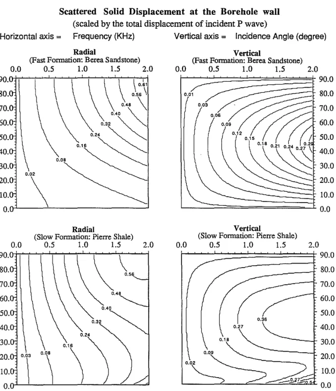
0), Figure 2 shows the radial and vertical component of the borehole scattered wave, scaled by the total displacement of the incident wave, I.e.,Ilu:(rb)ll/lla'h)11
and Ilu~h)ll/lla'h)ll, at the solid side of the borehole wall. For both hard and soft formations, the borehole scattered energy is negligible compared to the incident wave for a frequency below hundreds of Hertz (500 Hz for hard formation and 250 Hz for soft formation); while for a frequency above 1 kHz, the scattered energy is a significant portion of geophone output. For a frequency at 2 kHz, the radial component of the borehole scattered wave can reach almost 60% of incident total displacement at 90° incidence for both formations and the vertical component can reach 30% at 45° incidence for the hard formation and over 40% at 45° incidence and over 60% at grazing incidence for the soft formation. The radial component of the borehole scattered wave increases with frequency and incidence angle; the vertical component increases with frequency and incidence angle up to 45° then decreases with the increase of incidence angle.total displacement of the incident wave, i.e.,
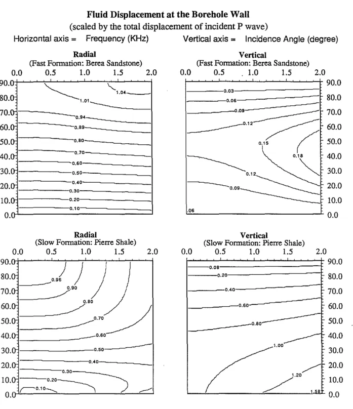
Ilu{(rb)ll/llit'h)11
andIlu{(rb)ll/llit'h)ll,
at the fluid side of the borehole wall. For the hard formation, the radial component of fluid displacement is almost independent of frequency except near 900 incidence andincreases rapidly with the increase of incidence angle; the vertical component is generally smaller (less than 20% of the total displacement) than the radial component and shows a peak at 450 incidence. For the soft formation, the radial component shows strong
frequency and incidence angle dependence in a complicated manner: it increases with frequency when the incidence angle is less than450 and decreases with frequency when
the incidence angle is greater than450
; the vertical component increases with frequency
and decreases with incidence angle and unlike the case of the hard formation the peak is at grazing incident rather than at 450
•
Figure 4 shows the pressure (amplitude and phase) at the center of the fluid scaled by the pressure of the incident P wave ( spherical component of the stress tensor), I.e., p/lpo, where Po
=
pa;lw)w
2(1 -i~:)Jo(kpr)
(see Lovell and Hornby, 1990 with correction), for both the hard and soft formations. For both cases the measured pressure at the fluid is much less than that if the borehole does not exist, which is due to the pressure release at the fluid-solid interface, especially for the hard formation. Generally, increase of frequency and incidence angle will increase the pressure at the fluid. The phase lag at the soft formation is less than that at the hard formation. It increases strongly with frequency and shows less dependence on the incidence angle except at the grazing incidence.Borehole Reception Pattern
The borehole reception pattern is defined as the ratio in amplitude of what we mea-sure to what we should meamea-sure if the borehole does not exist, i.e.,
Ilpfll/llpoll
for the pressure measurement,Ila/II/IIit'11
for the measurement of fluid displacement and(liaS +it'ID/IIit'11
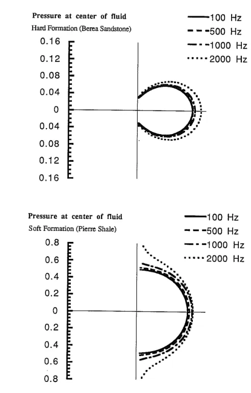
for the measurement of solid displacement (geophone output).Figure 5 shows the borehole reception pattern for pressure at the center of the fiuid at frequencies 100 Hz, 500 Hz, 1000 Hz and 2000 Hz. For the hard formation, the reception pattern shows a main lobe at 900 incidence (and is almost independent frequency) for
frequency below 1 kHz. For the soft formation, dependence on incidence angle is very weak compared to the previous case. At 2 kHz, the curve deflects toward the grazing incidence rather than the normal incidence.
Figure 6 shows the borehole reception pattern for the fluid displacement at the borehole wall. For the hard formation, the reception pattern shows little frequency dependence but strong incidence angle dependence with a main lobe at the 900 of
incidence angle and zero at grazing incidence. For the soft formation, the incidence angle dependence is much less significant than that in the hard formation for frequencies
below 1 kHz and the amplitude tends to be smaller at 90° incidence than that at grazing incidence, while for frequencies above 1 kHz, the reception pattern is more complicated with a valley at 90° incidence and two peaks at 45° and 135° incidences.
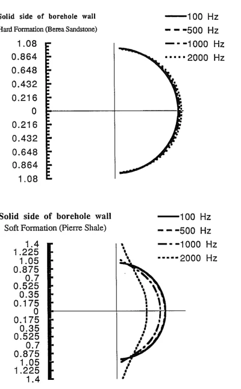
Figure 7 shows the borehole reception pattern for the solid displacement at the borehole wall. For the hard formation, the reception pattern is almost a unit circle with little frequency dependence. For the soft formation, the pattern looks the same as that for the hard formation for frequencies below 500 Hz, while for frequencies above 1 kHz, the amplitude at 90° incidence is significantly less than that at grazing incidence and frequency dependence is very strong.
Borehole Effect on Particle Motion
Since the displacement is a vector, the borehole distorts not only its amplitude but also its direction, i.e., particle motion. The estimation of particle motion is very important for data rotation of downhole 3-component measurements. It is beneficial if we can understand how and how much the borehole can change the polarization of particle displacement.
In this paper, inclination deviation is defined as the difference of the inclination (angle of displacement vector with the borehole axis) of measurement displacement from that of incident wave; azimuth deviation is defined as the difference of the azimuth angle of measured displacement from that of incident wave. Another important concept is the rectilinearity which is a measure of the nature of polarization (Esmersoy, 1984; Peng and Toksoz, 1991): for a perfect linear polarization the rectilinearity is 1 and for a perfect circular polarization it is zero.
Figure 8 shows the rectilinearity of displacement at the solid side of the borehole wall as a function of incidence angle at frequencies 100 Hz, 500 Hz, 1000 Hz and 2000 Hz. For the hard formation, the rectilinearity is very close to 1 which means the solid motion is linear, a little bit of the surface mode is excited at 2 kHz near grazing incidence. For the soft formation the frequency and incidence angle dependence is more obvious, although the particle motion is dominantly linear except at 2 kHz.
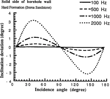
Figure 9 shows the inclination deviation for the displacement at the solid side of the borehole wall. For the hard formation, the inclination deviation is less than 1° for frequencies below 1 kHz and 3° at 2 kHz, the deviation is peaked at 45° and 135° incidence. For the soft formation, the inclination deviation tends to be larger than that for the hard formation and can reach 6° at grazing incidence at 2 kHz.
Effect of Geophone Orientation
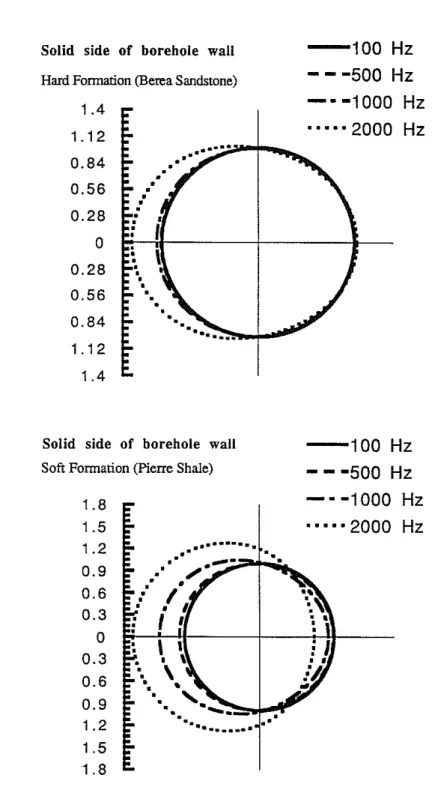
Because the problem is nonsymmetric in nature, the displacement and pressure will be dependent on the azimuth orientation of the geophone or hydrophone with respect to the incident wave. Figure 10 shows a polar plot of the calculation for a plane P wave incidence with incidence angle {j
=
45° and azimuth angle l/=
O. What we plot in this figure is the amplitude of solid displacement scaled by that of the incident wave (reception pattern) as a function of geophone azimuth anglee
(0°- 360°). For the hard formation, the reception pattern is independent of the geophone orientation for a frequency below 1 kHz, while for a frequency above 1 kHz, it has a large lobe at 180° azimuth angle (i.e, where the geophone is facing the incident wave which picks up the strong backscattered wave). For the soft formation the patterns look similar to those for the hard formation for frequencies below 500 Hz, while for a frequency above 500 Hz, the reception pattern is significantly less than unity in the forward scattering direction(0°) and is significantly larger than unity in the backward scattering direction (180°).
Figure 11 shows the inclination deviation of the solid displacement at the borehole wall as a function of geophone orientation angle
e
for a plane P wave incidence at{j
=
45°. For the hard formation, the deviation is less than 3° and for the soft formationit can reach 4° in the forward scattering direction.
Figure 12 shows the azimuth deviation of the solid displacement at the borehole wall. At low frequencies the deviations are almost zero, but at 2 kHz it can reach 6° when the geophone is at 90° or 270° azimuth for the hard formation, and 15° when the geophone is at 45° or 315° azimuth for the soft formation.
SHEAR PLANE WAVE INCIDENCE
The interaction of the shear wave (SV type) with the fluid-filled borehole is more com-plicated than the case of P incidence. Mode conversion and possible excitation of the surface wave (e.g., tube wave) occur at the interface, which makes the effect of the borehole coupling more significant.
Frequency and Incidence Angle Dependence
Figure 13 shows the radial and vertical components of the borehole scattered wave,
scaled by the total displacement of the incident wave, i.e.,
Ilu:(rb)II/IIUih)11
andIlu;h)II/IIUi(rb)ll,
at the solid side of the borehole wall with the geophone orientatione
= 0). The incidentwave is of SV type plane wave with azimuthl/
=
O. For the hard formation, the borehole scattered energy is negligible at low frequencies, while at high frequencies the scatteredwave can be a significant portion of the total measurement. The radial component of the borehole scattered wave increases with frequency and decreases with the incidence angle, while the vertical component of the scattered wave shows a minimum at 450
in-cidence and has two peaks at grazing inin-cidence and normal inin-cidence. For a frequency around 2 kHz, the radial component of the borehole scattered wave can reach almost 110% of incident total displacement at grazing incidence and the vertical component can reach 70% at 00 incidence and 50% at normal incidence. For the soft formation,
strong resonances in the fluid occur at low frequencies and certain incidence angle where the vertical wavenumber
(w/
f3
cos 6 ) is equal to the tube wave wavenumber (w/
CT ) at which the tube wave is excited. At that particular frequency and incidence angle, the scattered wave can be several times larger than the incident wave. Away from the resonance region, the frequency and incidence angle dependence is similar to that for the hard formation.Figure 14 shows the radial and vertical components of fluid displacement scaled by the total displacement of incident wave, i.e.,
Iluth)II/IIiI'h)11
andIlu{h)II/IIiI'(rb)ll,
at the fluid side of the borehole wall. For the hard formation, the radial component of fluid displacement is almost independent of frequency except near 0° incidence and increases rapidly with the decrease of incidence angle; the vertical component is smaller in magnitude than the radial component and at high frequencies it shows a peak at 0° incidence. For the soft formation, significant fluid resonance is also observed at low frequencies and certain incidence angle. Away from the resonance region, the radial component shows complicated frequency dependence: it first decreases with frequency, reaches a minimum around 1 kHz (depending on the incidence angle) then increases again. Generally the radial component decreases with the increase of incidence angle. The vertical component shows almost no frequency when the incidence angle is above 400 and increase of incidence angle will decrease its amplitude.Figure 15 shows the pressure (amplitude and phase) at the center of the fluid scaled by Po = pf3'(;JWlw2Jo(ksr). For the hard formation and an incidence angle above 400
the amplitude shows no dependence on frequency and for an incidence angle below 40° significant frequency dependence can be observed. The amplitude increases with the decrease of incidence angle. The phase lag for the hard formation shows strong frequency and incidence angle dependence. For the soft formation, the pressure resonance is more significant at low frequencies and certain angles of incidence. Away from the resonance region, the amplitude is almost independent of frequency for normal incidence. The phase lag shows much complicated frequency and incidence dependence.
The angle at which resonance occurs can be theoretically predicted at a given fre-quency. From the tube wave dispersion equation, we can derive the analytical expression for the tube wave phase velocity at low frequency approximation. Up to the order w2lnw (neglecting terms of order w4ln
w
or higher), the tube wave phase velocity can be writtenGT=
as
af [1_1 pfa} (1_ 2,82 _2Pf)(1_2,82)w2n2JnwTb]
1
+
Pfa; 4p,82+
Pfa} a} P a2 ,82 2ap,8
which agrees with the result of Biot (1952) and White (1983) as W --->
o.
(9)
Figure 16a shows the frequency dependence of the tube wave phase velocity for soft formation (Pierre shale). For a frequency below 1 kHz, GT
>
,8; and for a frequency above the cut-off, GT<
,8.The resonance occurs at ~cos/j = ~, so we have
/j
=
cos-1L
(10)GT
which has solution only whenGT
>
,8, which implies that the borehole resonance is a low frequency phenomenon.Figure 16b shows the comparison of the prediction of resonance angle under low frequency approximation with that of exact solution. Excellent agreement can be found at frequencies below 400 Hz.
For an plane SH wave incidence, the wave fields inside and outside the borehole turned out to be much simpler owing to the fact that SH motion is not coupled with P or SV motion. Figure 17 shows the transverse components of fiuid and scattered solid displacement at the borehole wall scaled by the total displacement of incident SH wave, Le., Ilu~(Tb)II/IIUih)11 and
Ilu(jh)II/IIUih)ll.
For the fast formation, the displacement in the fiuid is strongly dependent on frequency, but almost independent of incidence angle at low frequencies. At high frequency the angle dependence is more significant. At 2 kHz and grazing incidence, the fiuid displacement reaches 160% of the incident wave. For the soft formation, the displacement in the fiuid depends on both frequency and incidence angle. Contrary to what we might expect, in this case increase of frequency will decrease the fluid displacement. There is a peak around 600 Hz and grazing incidence. The displacement of the scattered wave in the solid increases with frequency and incidence angle in the fast formation. At 2 kHz and 900 incidence it canreach 70% of the displacement of the incident wave. In the soft formation, the scattered wave shows similar behaviour as that in the fast formation. At 2 kHz and900
incidence it can reach 100% of the displacement of the incident wave.
Borehole Reception Pattern
Figure 18 shows the borehole reception pattern for pressure, i.e.,
Ilpfll/llpoll,
at the center of fluid at frequencies 100 Hz, 500 Hz, 1000 Hz and 2000 Hz for a plane SV waveincidence. For the hard formation, the reception pattern shows two lobes at 450 and
1350 incidence and is almost independent of frequency for frequency below 1 kHz. The
pressure at the center of the fluid is zero at normal incidence and very small at grazing incidence. For the soft formation, large fluid resonance occurs at250 at 100 Hz and 20°
at 500 Hz. For frequencies above 1 kHz, the fluid resonance disappears. The reception pattern shows strong and complicated frequency and incidence angle dependence.
Figure 19 shows the borehole reception pattern for the fluid displacement, I.e.,
Ilu/II/IIUiII,
at the borehole wall for a plane SV incidence. For the hard formation, the reception pattern shows little frequency dependence but strong incidence angle de-pendence with a main lobe at the 00 incidence and zero at 900 incidence. For the softformation, similar to the corresponding pressure reception pattern, strong resonance of fluid motion occurs at low frequencies and small incidence angle. For frequencies above 1 kHz no resonance occurs, but the reception pattern shows very complicated behaviour. For example, at 2 kHz, the reception pattern has four lobes. For all the cases, the fluid motion is zero at 900 incidence.
Figure 20 shows the borehole reception pattern for the solid displacement, i.e.,
(1Iu
s+
1711)/111711,
at the borehole wall for a plane SV incidence. For the hard formation, the reception pattern is almost a unit circle with little frequency dependence except at 2 kHz. For the soft formation, the resonance is very weak compared to that in the fluid at low frequencies and small incidence angles. In this case, the reception pattern shows strong dependence on frequency and incidence angle. Generally the solid displacement is smaller than that of the incident wave at around normal incidence and is larger around grazing incidence, especially at high frequencies.Figure 21 shows the borehole reception pattern for the fluid displacement at the borehole wall for a plane SH wave incidence. For the hard formation, the reception pattern is nearly a unit circle except at 2 kHz. For the soft formation, although no resonance occurs, the reception pattern at low frequencies is quite different from that at high frequencies. At low frequencies, the pattern is a unit circle; at high frequencies it has two lobes around 200 and
1600 incidence and valleys at both normal and grazing
incidences.
Figure 22 shows the borehole reception pattern for the solid displacement at the borehole wall for a plane SH wave incidence. For the hard formation, the reception pattern is nearly a unit circle except at 2 kHz. For the soft formation, at frequencies below 1 kHz the reception pattern is also nearly a unit circle, while at frequencies above 1 kHz three lobes at 200
, 900 and 1600 are obvious.
Borehole Effect on Particle Motion
Figure 23 shows the rectilinearity of displacement at the solid side of the borehole wall as a function of incidence angle at frequencies 100 Hz, 500 Hz, 1000 Hz and 2000 Hz for a plane SV incidence. For the hard formation, the rectilinearity is very close to 1 except at 2 kHz near grazing incidence. For the soft formation the frequency and incidence angle dependence is more obvious, although the particle motion is dominantly linear except where the tube wave is excited at low frequencies and where some leaking modes appear at high frequencies.
Figure 24 shows the inclination deviation for the displacement at the solid side of the borehole wall for a plane SV incidence. For the hard formation, the inclination deviation is less than 1° for frequencies below 1 kHz and 3° at 2 kHz. For the soft formation, the inclination deviation can reach 20° at low frequency near the fluid resonance angle. For frequencies above 1 kHz, significant deviation of particle motion occurs in the soft formation.
Effect of Geophone Orientation
Figure 25 shows a polar plot of the calculation for a plane SV wave incidence with incidence angle 0= 45°and azimuth angle 1/= O. Plotted here is the amplitude of solid displacement scaled by that of the incident wave (reception pattern) as a function of geophone azimuth angle () (0°- 360°). For the hard formation, the reception pattern is independent of the geophone orientation for frequencies below 1 kHz, while for frequen-cies above 1 kHz it has a large lobe at 180° azimuth angle (i.e, the geophone is facing the incident wave). For the soft formation the pattern looks similar to that for the hard formation for frequencies below 100 Hz, while for frequencies between 100 - 500 Hz, the reception pattern is less than unity in the forward scattering direction (0°) and pretty much the same in the backward direction. For frequencies above 500 Hz, the pattern is significantly less than unity in the forward direction and significantly larger than unity in the backward scattering direction (180°).
Figure 26 shows the same polar plot as in Figure 25 except for SH wave incidence. For the hard formation, the reception pattern for SH incidence is nearly a unit circle for frequencies below 1 kHz and for a frequency above 1 kHz it also has a large lobe at 180° azimuth angle. For the soft formation the pattern looks similar to that for the hard formation for frequencies below 500 Hz, and for a frequency around 1 kHz, the reception pattern has a large lobe at 180° azimuth, while for frequency around 2 kHz the main lobes occur at 90° and 270° azimuths.
Figure 27 shows the inclination deviation of the solid displacement at the borehole wall as a function of geophone orientation angle () for a plane SV wave incidence at
8= 450
• For the hard formation, the deviation can reach II
°
and for the soft formationit can reach 70° in the forward scattering direction at 2 kHz.
Figure 28 shows the azimuth deviation of the solid displacement at the borehole wall for a plane SV incidence. At low frequencies the deviation is almost zero, but at 2 kHz it can reach 100when the geophone is at 1000or2600azimuth for the hard formation, and 1000when the geophone is around 00 azimuth for the soft formation.
DISCUSSION AND CONCLUSIONS
In this paper, we have presented an exact formulation for borehole coupling based on Schoenberg's theory, which is valid for all frequency and all azimuthally symmetric and nonsymmetric components. We have studied the borehole effects on downhole seismic measurements (both in amplitude and particle motion) as functions of frequency, incidence angle and polarization of incident wave as well as the geophone orientation. We found
• For the hard formation and frequency below 500 Hz, the borehole scattered energy in the solid is less than 10
%
in amplitude of the incident wave and the downhole geophone measurement is nearly not affected by the fluid-filled borehole. Although frequency plays a less significant role in this case, the pressure measured at the center of the fluid is strongly dependent on the direction of incidence wave, e.g., for a P wave incidence the pressure reception pattern has a big lobe around normal incidence and for an SY incidence it has two lobes at 45° and 135° incidence. • For the hard formation and frequency above 500 Hz, especially on the order of 1kHz, the borehole scattered energy is a significant part of the total measurement of the downhole geophone for any type of incident wave. The particle motion direc-tion can be different from that of the incoming wave by several degrees depending on the incidence direction and frequency. The solid displacement measured with the geophone facing the incoming wave will be noticibly larger than that with the geophone opposite. The pressure at the center of the fluid shows dependence on frequency as well as incidence angle.
• For the soft formation and frequency below above 300 - 500 Hertz, the borehole scattered energy in the solid is also negligible for a P-wave incidence, and in this case the pressure at the center of the fluid becomes significantly less dependent on incidence angle as it does in the hard formation. For an SY wave incidence, significant fluid resonance occurs at certain incidence angles for frequencies below 1 kHz due to the excitation of the tube wave. At these particuiar frequencies and incidence angles, the solid displacement measured by the downhole geophone and pressure picked by the downhole hydrophone will be several times larger than those of the incident wave, the particle motion from geophone measurements differs from that of the incident wave by as large as 20°.
• For the soft formation and frequency above 1 kHz, the fluid resonance disap-pears for SY incidence. In this case, the solid displacement and fluid pressure are strongly dependent on both frequency and incidence angle in a complicated man-ner. For a P-wave incidence, the displacement in the solid is smaller than that of the incidence wave at normal incidence and is significantly larger at grazing inci-dence. Also the measured solid displacement is much larger than the incident wave
when the geophone is facing the incident wave and is smaller when the geophone is opposite to it.
We conclude that correction of the borehole effect for downhole measurements should be made for frequencies above 500Hzin the hard formation. In the soft formation, if the incidence angle is well away from the resonance angle for an SV incidence, no borehole correction is needed for frequencies below 300 Hz; for frequencies above 300 Hz, the borehole can cause severe problems on downhole measurements and proper attention to this effect should be taken. Since the borehole can significantly alter the particle motion direction, horizontal components rotation from data itself is unreliable for experiments with frequencies above 1 kHz and rotation should be done from downhole gyro readings if possible.
A frequency-wavenumber filter can be designed to remove the borehole corruption to the measured data so that the true amplitude of the incident wave can be restored. This can be achieved by inverting the borehole coupling filter using the Wiener-Levinson algorithm (Robinson, 1967). This will be a subject of further study.
ACKNOWLEDGMENTS
This work was sponsored by the ERL/nCUBE Geophysical Center for Parallel Pre-cessing and the Borehole Acoustics and Logging Consortium at the Earth Resources Laboratory, MIT. The first author holds an nCUBE fellowship. We are grateful for helpful discussions with Dr Roger Turpening and Dr Zhenya Zhu.
REFERENCES
Biot, M., 1952, Propagation of elastic waves in a cylindrical borehole containing a fluid, J. Appl. Phys., 23,997-1009.
Bregman, N.D., R.C. Bailey, and C.H. Chapman, 1989, Crosshole seismic tomography, Geophysics, 54, 200-215.
Esmersoy, C., 1984, Polarization analysis, rotation and velocity estimation in three component VSP, in Vertical Seismic Profiling, 14B, 236-255.
Harris, J.M., 1988, Cross-well seismic measurements in sedimentary rocks, 58th Ann. Intemat. Mtg., Soc. Expl. Geophys., Expanded abstracts, 147-150.
Lovell, J.R.and Hornby, B. E., 1990, Borehole coupling at sonic frequencies, Geophysics,
55, 806-814.
Peng, C. and M.N. ToksGz, 1992, Vector seismic array processing with application to crosshole/VSP data, to be submitted to J. Seismic Exploration.
Robinson, E.A. and S. Treitel, 1980, Geophysical Signal Processing, Prentice Hall, En-glewood Clifs, N. J.
Schoenberg, M., 1986, Fluid and solid motion on the neighborhood of a fluid-filled borehole due to the passage of a low frequency elastic plane wave, Geophysics, 51, 1191-1205.
Timoshenko, S. and J.N. Goodier, 1951, Theory of Elasticity, McGraw-Hill, New York. Tura, M.A.C, 1991, Application of diffraction tomography to fracture detection, 61st
Ann. Intemat. Mtg., Soc. Expl. Geophys., Expanded abstracts, 836-839.
White, J.E., 1953, Signals in a borehole due to plane waves in the solid, J. Acoust. Soc. Amer., 25, 906-915.
Appendix A.
BASIC EQUATIONS IN CYLINDRICAL
COORDINATE
In terms of four potentials t/>j, t/>, ~ and ,p, the displacement and stress can be written as
Uj
-
e• ot/>jr or+
eO-:;: 00• lot/>j+
e• ot/>jz ozot/> 02~ lo,p Ur
-
- + - - + - -
or oroz roO lot/> 1 02~a,p
UO =+
-r 00 r oOoz or Uz - ot/>oz+
OZ202~
_\72~
and 2 2 lot/> 1 02t/> 02t/> 0 w2 1o~ 1 02~ 02~arr - -pw t/>-2pfJ [(-:;:or
+
r2002+
OZ2)+oZ(fJ2~+-:;:or
+
r 2 002+
OZ2)1 o,p 1 02,p
+
r2 00 - -:;: oroOI2 02t/> 0 w2 02~ 1 02,p
arz 2pfJ [oroz
+
or(2fJ2~+
OZ2)+
2rozoO I2 0 1ot/> t/> 02 1o~ ~ 1 02,p 1o,p 1 w2 02,p
aro
=
2pfJ [00(-:;: or - r 2)+
ozoO(-:;: or - r 2)+
r2 002+ -:;:
or+
2"(fJ2,p+
Oz2)]and
azz
=
azO
aOO
=
\
Except for the displacement and stress components given before, those components that are not explicitly involved in the boundary conditions are as follows
u~
-ar:a
W
)
[Ubo(r)Ao+ 2'L':'=linUbn (r)( -Ansin nO+A~cosnO)]
u¢ --
a~~w)
[Uta(r)Bo + 2'L':'=linutn(r)( -Bnsin nO+B~cosnO)]
0
u~
--
f1~~W) [U~o(r)Go
+ 2'L':'=linU~n
(r)(-GnsinnO+G~cosnO)]
u'l/J --
f1~~W) [Uta(r)D~
+ 2'L':'=
lin U't (r)(-DnsinnO+D~cos
nO)]0
ufz
ar:a
W
)
[U!o(r)Ao+ 2'L':'=linufn(r) (Ancos nO+A~sin
nO)] u¢ =-
a~(jV)
[U1o(r)Bo+ 2'L':'=linu!n (r) (Bncos nO+B~sin
nO)]z
u~z
_,6~~W)
[U;o(r)Go + 2'L':'=linU;n(r) (Gncos nO+G~sin
nO)] u'l/Jz = 0and
¢
pa:Jw)
[.c¢o(r)Bo+2'L':'=lin .c¢n(r)(BncosnO
+
B~sinnO)] (jzz~
Pf1:JW) [
.c~o(r)Go
+ 2'L':'=lin.c~n(r)(GncosnO
+G~sin
nO)](j zz
'l/J
0 (j zz¢
pa:Jw)
[M¢o(r)Bo + 2'L~lin M¢n(r)(BncosnO + B~sin nO)](j00
-~
p,6~JW) [M~o(r)Go
+ 2'L':'=linM~n(r)(GncosnO
+~sin
nO)](j00
'l/J
p,6~JW)
[
M'l/Jo(r)Do+ 2'L':'=lin M'l/Jn (r)(DncosnO+D~sin
nO)](j00
pa~JW) [N¢o(r)B~
+
2'L':'=lin N ¢n(r) (-BnsinnO+
B~cosnO)]Pf1:JW)
[N~o(r)G~ +
2'L':'=linN~n(r)(
-GnsinnO+
G~cosnO)]
p,6:JW) [
N'l/Jo(r)D~
+
2'L':'=lin N 'l/Jn(r)(-DnsinnO+
D~cos
nO)). Given below are lists of coefficients in the expressions for stress and displacements:U!n(r) = kfJ~(kfr), ¢ ( I ) ' ) Urn(r) = kpHn (kpr, U
g
¢ (r)=
I;,nH~I\kpr),
nI;;
U!"(r) =ikzH~I)(kpr),
Rfn(r) = -w2Jn(kfr)R¢n(r) = _[(w2 -
2{32kz2)H~I)(kpr)
+
2{3;;p2(H~I)'
(kpr) _~H~I)(kpr))]
Ren(r) =2kzZ~2!r [H~I)(ksr)
+
f.;H~I)'
(ksr) -k~;r2H~I)(ksr)]
RI. (r)
=
-2{32k/n[~1H~I)(ksr) - -,:LH~I)' (ksr)]lPn s r2 l'i;ST
GA._(r) = -2{32kp2n[z;-hH~I)(kpr) - -,:LH~I)'(kpr)]
!pH rvp r2 fl-pT
Gen(r) =
2kzZ~2(t n[k}r2H~I)(ksr)
-f.;H~I)'
(ksr)]Gol'n(r)
=
-(32ks2[H~I)(ksr)+
.;}-H~I)' (ksr) - k21\H~I)(ksr))~ l'i;sr s r
( ) . 2 (I)' ( Z¢n r
=
2~kzkp{3 Hn kpr) Zener)=
_i(kz2-t~)ks{32 H~I)'
(ksr) Z'lj;n(r) =ikzks{32f;;.H~I\ksr)
£¢n(r) = _[w2 - 2{32(ka 2 - k/)]H~I)(kpr) £en(r) =
-2{32~(ki
- kz2)H~I)
(ksr){3 £'lj;n (r)
=
0 MA. (r)=
_(0:2 - 2(32)k0:2H~l)
(kpr)+
2{32 1;,2H~l)'
(kpr) _ 2{32kk~
2 n 2H~l}
(kpr) ~ ~ pr2Men(r)
=
-2{32~{3[~H~I)'
(ksr) -kk~22 n2H~I)(ksr))
s s r Mol'n(r) = 2{32ks2n[k ~ 2H~l}(ksr) - .,LH~I)'(ksr)] r.p s r /'1;ST N¢n(r)
=
2i{32T;
PnH2) (kpr) k 2 2k 2 N (r) - i{32 (3 - z.0-
n H(I)(k r) en - ksr Ie(3 n sN
'lj;n r()
=
~kzks{3.
2Hn(1)'(ksr)where ka
=
~,
kf3=
W,
kp=
Jka2- kz2, k s=
J k l - k z2 and kf=
J~
-
kz2• kz=
ka cos 0 for plane P wave incidence and kz=
kf3cos 0 for plane shear wave inci-dence. 0is the incidence angle.Appendix B.
STRESS AND DISPLACEMENT OF INCIDENT
PLANE WAVE
For a plane P wave traveling in the direction
~ =
(sin o cos v,sinosinv, coso), where 0 is the incidence angle with respect to the borehole axis and v is the a2imuth angle, the displacement potential can be written as (omitting ei(kzz-wt) dependence)<pp
-
a~~w) exp[ikpr cos(O - v)] (B-1)=
_a~~w) [Jo(kpr) +2 L:::"=lin(cosnvcosnO + sinnvsinnO)Jn(kpr)]. In addition to the displacement and stress components given in (4), we haveu~
=
_a~<,w) [USo(r) +2 L:::"=linUSn(r)(-cosnvsinnO + sinnvcosnO)]- a~~w) [U:O(r)
+
2 L:::"=linUI,,(r)(cos nv cos nO+
sin nv sin nO)]. Ifthe incident plane wave is of SV type, the displacement potential will beCsv
=
iltV(w) I ['k (0)1
(B-2)(". w 3 . s: expz srcos - v
Slllu
- if3';3(W)
~
[Jo(ksr)+
2 L:::"=lin(cos nv cos nO+
sin nv sin nO)Jn(ksr)1 andu~v
=_§~~W)
[U3tY(r)+
2 L:::"=linUS'; (r) (- cosnv sinnO+
sin nv cos nO)]u~v
=_§~~W)
[U:cnr) +2L:::"=linU;'';(r)(cosnvcosnO+sinnvsinnO)].Similarly, for a plane SH wave incidence
f3V(W) I .
'l/JSH = ---wz-~ exp[tksrcos(O - v)] (B-3)
Slllu
and
U~H
_ _13:S
W) [Ug:(r) +2 I::;"=linug:(r)(cosnvcosne + sinnvsinne)]u~H _ O.
The coefficients are given below
UeP (r)
=
Iv"
In(kpr), U!:.(r)=
ik.Jn(kpr)n ~
UeSV (r)
=
-liz.-nJn(ksr), uf: (r)=
iksJn(ksr)n fesT Ug:(r) = -k{3J~(ksr), UfnH(r) = 0 Rpn(r) = _[(w2 - 2{32kz2)Jn(kpr)
+
2{321v,,2(J~(kpr)
- -?-In(kpr))]f;;
r.;pT 8Pn(r)=
-2{32kp2n[z.1
In(kpr) - -!::J~(kpr)] np r2 n-pT ZPn(r)=
2i{32k.kpJ~(kpr) Rsvn(r)=
2{32k.ksPn(ksr)+
.,LJ~(ksr)
- kn; In(ksr)] /'l;sT s r2 8svn(r)=
-2{32ksk.n[.,LJ~(ksr) -k"""l
In(ksr)] /l,sT s r 2 ZSVn(r) = i{32(ks2- k.2)J~(ksr)z axis
t
1U
k
x axis
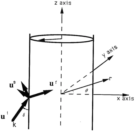
Figure 1: A fluid-filled borehole (af,Pf) in a solid formation (a,fJ,p). An elastic wave
U'
incident on the borehole which causes scattered wave ils in the formation and fluid motion ilf in the borehole. The borehole radius isTb. The incidence angle is /jScattered Solid Displacement at the Borehole wall
(scaledbythe total displacement of incident P wave)Horizontal axis= Frequency (KHz) Vertical axis= Incidence Angle (degree)
Radial
(Fast Fonnation: Berea Sandstone)
0.5 1.0 1.5 2.0
Vertical
(Fast Fonnation: Berea Sandstone)
0.5 1.0 1.5 0.0 0.0
:~:O:h-'---'--t---'--t--'-'-~\'T"'"""'-\"""""""\0;'-7\\5:'~\
0.48 \ 70. 60. 50. 0.16 40. 0.08 30. 20. 10, O , n . L - - - ' - - - . J 0.36 0.27 0.18 0.09 0.02 2.0 I~-:::~:::=:==::::::::=====t90.0 80.0 ~---E-70.0 60.0 50,0 40.0--...J:.
30.0 20.0 10.0 '- -4._ _.c:.=--'"""~...-:=~:::.-",':.MCL 0.0 Vertical(Slow Fonnation: Pierre Shale)
0.0 0.5 1.0 1.5
0.40
0.24
Radial
(Slow Fonnation: Pierre Shale)
0.5 1.0 1.5 2.0 0.0 90.0:/-;--c-...,...l.;---';-...J...,...\~...,\~~ 80.
~
os. 0.48 20.Figure 2: The radial and vertical components of the borehole scattered wave scaled by the total displacement of incident wave for hard (top) and soft (bottom) formations. The incident wave is a plane P wave with v
=
O. The geophone is at (r=
rb, ()=
0)Fluid Displacement at the Borehole Wall
(scaledbythe total displacement of incident P wave)
Horizontal axis= Frequency (KHz) Vertical axis= Incidence Angle (degree)
Vertical
(Fast Formation: Berea Sandstone)
0.5 . 1.0 1.5 70.0 60.0 50.0 40.0 30.0 20.0 10.0 !:l:·o::.6 .J. 0.0 2.0 I-'-~-'--'-~~...L.~~--l..,.,~~+90.0
1----0.03---F
,
0.06
-
80.0,-
O.09-~---______0.12 / /
015 ( ~ 0.1.___
0.'2~ ~
0.09~ 0.0 Radial(Fast Formation: Berea Sandstone)
0.5 1.0 1.5 2.0 u
~
",.04_
0- 1.01 _ _ _ _ _ _ _ _ _ _ _ _ .v· ...0.94_.li
0.89_.CT
0.80_.li
0.70 0.60'"
.V 0.50.CT
0.40 0.30 .u. 0.20 0.10 .IF 0.0 90. 80. 70 60 50 40 30 20 10o
2.0 90.0 80.0 70.0 60.0 50.0 40.0 30.0 20.0 10.0 0.0 Vertical(Slow Formation: Pierre Shale)
0.5 1.0 1.5 0.08 0.20 0.40 0.60 _ o . 8 0
-/20
1"oj 0.0 Radial(Slow Formation: Pierre Shale)
0.5 1.0 1.5 2.0 v
~})
0-li
- - - : : : : 0 . 7 0
~
li
.li
. - - 0 . 6 0CT
0 . 5 0-li
DADO"~
u-: 0.20r-O.10--...~
---.V 0.0 90. 80. 70. 60. 50. 40. 30. 20. 10.o
Figure 3: The radial and vertical components of fluid displacement at (r = rb'
e
= 0) scaled by the total displacement of the incident wave for hard (top) and soft (bottom) formations. The incident wave is a plane P wave with v =o.
Horizontal axis
=
Pressure at the Center of Fluid
(scaledbythe pressure of incident P wave)
Frequency (KHz) Vertical axis = Incidence Angle (degree)
O . n - L - - - '
Amplitude
(Fast Formation: Berea Sandstone)
0.5 1.0 1.5
Phase
(Fast Formation: Berea Sandstone)
0.5 1.0 1.5 2.0 I-'--..,...-'-I-~...-'-i-~,...--';-~..,...+90.0 80.0 70.0 60.0
I
50.0.1
40.040.00 46.00 56( 64C
,'~~'~:
0.0 0.0 0.0 90.O+-~~--'--'~""""T-'---'-~~';-'-~-'rI 80. 70. Amplitude(Slow Formation: Pierre Shale)
0.5 1.0 1.5 2.0
4.00
Phase
(Slow Formation: Pierre Shale)
0.5 1.0 1.5 2.0
\
\
I
90.0".0:2.
00'6.\66
~~:~
60.0 50.0 40.080\ \
~~:~
' - ' \,,~
10.0 '--_-"-_---"_--''----'----'---'---'-.!L 0.0 0.0 0.0 90.rrJ--';-~~'-'-~..,...L..._'_t~_'_7'~-t-'~Ti 80. \ \~76
0.\
70. \ \:
0.' .. O'\\::
40. ""~
30. 20. 10. ../ ____ O."
~ '_--'---'---<:::...<:::...="""~:==:~::2:~~Figure 4: Pressure at the center of the fluid scaled byPo (see text), the pressure of the incident P wave, for hard (top) and soft (bottom) formations.
Pressure at center of fluid
Hard Formation (Berea Sandstone)
0.16
0.12
0.08
0.04
o
0.04
0.08
0.12
0.16
Pressure at center of fluid
Soft Formation (Pierre Shale)
0.8
0.6
0.4
0.2
o
0.2
0.4
0.6
0.8
- 1 0 0 Hz
- - -500 Hz
_ . -1000 Hz
···2000 Hz
- 1 0 0 Hz
- - -500 Hz
_ . -1000 Hz
... 2000 Hz
Figure 5: Borehole reception pattern for pressure at the center of the fluid at frequencies 100 Hz, 500 Hz, 1000 Hz and 2000 Hz for hard (top) and soft (bottom) formations. The incident wave is a plane P wave with v
=
o.
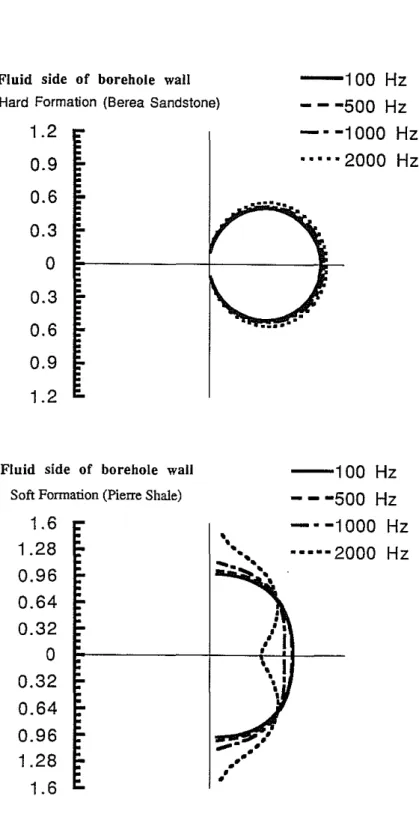
Fluid side of borehole wall
Hard Formation (Berea Sandstone)
1.2
0.9
0.6
0.3
o
0.3
0.6
0.9
1.2
- 1 0 0 Hz
- - -500 Hz
_ . -1000 Hz
... 2000 Hz
- 1 0 0 Hz
- - -500 Hz
_ . -1000 Hz
···2000
Hz
"",..-.-'
•
.'
•
•
•
1.6
1.28
0.96
0.64
0.32
o
0.32
0.64
0.96
1.28
1.6
Fluid side of borehole wall
Soft Formation (Pierre Shale)
Figure 6: Borehole reception pattern for fluid displacement at (r = r;,
e
= 0) at frequencies 100 Hz, 500 Hz, 1000 Hz and 2000 Hz for hard (top) and soft (bottom) formations. The incident wave is a plane P wave with v=
O.- 1 0 0 Hz
- - -500 Hz
_ . -1000 Hz
···2000 Hz
Solid side of borehole wall
Hard Fonnation (Berea Sandstone)
1.08
0.864
0.648
0.432
0.216
o
0.216
0.432
0.648
0.864
1.08
Solid side of borehole wall Soft Formation (Pierre Shale)
1.4
1.225
1.05
0.875
0.7
0.525
0.35
0.175
o
0.175
0.35
0.525
0.7
0.875
1.05
1.225
1.4
- 1 0 0 Hz
- - -500 Hz
_ . -1000 Hz
···2000
Hz
Figure 7: Borehole reception pattern for solid displacement at frequencies 100 Hz, 500 Hz, 1000 Hz and 2000 Hz for hard (top) and soft (bottom) formations. The incident wave is a plane P wave with 1I= O. The geophone is at (r = rt,rJ = 0).
- 1 0 0 Hz - - -500 Hz - - -1000 Hz -=,-.-,::oo~,....----""=":"-~...',",,'...2000 Hz t""Oi
. > .
-..
. ,
=_,
.
-.. -II ' .··
.
/
~.
l
\
.
~.
·
.
·
.
··· .
I. .. II .. ',' ',-0.99 0.992Solid side of borehole wall Hard Fonnation (Berea Sandstone)
1.002 0.998 ~ ';: 1ll 0.996
a
tl 0.994 ~ 180 O. 988.L..L.l...I..I.J...u...
L1.I~...:.u...u...
uJo
30 60 90 120 150Incidence angle (degree)
Solid side of borehole wall
Soft Formation (Pierre Shale)
--
.
/
• .." 1.02 0.98 >, 0.96 -.;:..
"
0.94a
tl 0.92"
"
0.9 0.88·.
..
.
·
·
·.
..
.
:
.
..
.
.
.
----
.
.
,.
..
.'
' I I, - -•.
.
..
'.
- 1 0 0 Hz - - -500 Hz - - -1000 Hz ... 2000 Hz 0.86 ~"""":':'''''''.u.JLL.&''''''L.1.I~""",...u...
uJo
30 60 90 120 150 180Incidence angle (degree)
. Figure 8: Rectilinearity for the solid displacement at frequencies 100 Hz, 500 Hz, 1000 Hz and 2000 Hz for hard (top) and soft (bottom) formations. The incident wave is a plane P wave with v = O. The geophone is at (r = ri,",
e
= 0).30 60 90 120 150 180
Incidence angle (degree)
Solid side of borehole wall
HardFonnation (Berea Sandstone) 4 0;- 3
'"...
2 on'"
:::,
c 0 :ca
'"
.;;:'"
'C - 1 c 0 :c - 2'"
.5 <:i - 3 c-
- 4a
.'.
.
,.
.
It ..'..1 " . - ... I.
: • . . I I ---~. - 1 0 0 Hz - --500 Hz ---1000 Hz .•••• 2000 Hz "I ... - - - / : ". ....
.. I I.
. . . , ..-.
.
.
.
' ,.
.
.
.
,.
.
,.'
'..
Solid side of borehole wall Soft Formation (pierre Shale)
1
a
0;-6'"
...
on'"
:::, c 2 .51 -; .;;:'"
- 2 'C c .51 -; - 6 c:s
c-
- 1a
a
- 1 0 0 Hz - - -500 Hz _ . -1000 Hz ... 2000 Hz.
I I " .. . . . . .. ,.
.,it. - __ ".... •.
..--....
..,-..--=-
--~ 0 ' 30 60 90 120 150 180Incidence angle (degree)
Figure 9: Inclination deviation from the incident wave for the solid displacement at frequencies 100 Hz, 500 Hz, 1000 Hz and 2000 Hz for hard (top) and soft (bottom) formations. The incident wave is a plane P wave with v
=
O. The geophone is at (r=
rt,
e
=
0).Solid side of borehole wall Hard Fonnarion (Berea Sandstone)
- 1 0 0 Hz
- - -500 Hz
- - -1000 Hz
••••• 2000 Hz
••• -:';';;0'-1-oO!-..
...
.
•.
• •··
·
••·
•• •• ••.
..
". •• . ;::'\0_... -1.4 1.12 0.84 0.56 0.28o
0.28 0.56 0.84 1.12 1.4Solid side of borehole wall Soft Formation (Pierre Shale)
1.8 1.5 1.2 0.9 0.6 0.3
o
0.3 0.6 0.9 1.2 1.5 1.8- 1 0 0 Hz
- - -500 Hz
- - -1000 Hz
... 2000 Hz
(Figure 10: Effect of geophone orientation on the borehole reception pattern at fre-quencies 100 Hz, 500 Hz, 1000 Hz and 2000 Hz for hard (top) and soft (bottom) formations. The incident wave is a plane P wave with {j
=
45 and lJ=
O. Thegeophone is at
r
=rt-
e
varies from 00.
---,
:--._--_.--:
.."..
.
.."..
Solid side of borehole wall
HardFonnation(Berea Sandstone)
4 ,
.
,, ,.
---
---:
----~
- 1 0 0 Hz - - -500 Hz - - -1000 Hz ••••• 2000 Hz.
, .' " , , , ,--,
--t-
,
• ""...
- 2 _1-J...--L-:-':---1--L-~.L....J...--L-':---1--L-.&...Jo
90 180 270 360Geophone orientation (degree)
."
...
.
,, , , , , i / ' - ' :. - 1 0 0 Hz - - -500 Hz - - -1000 Hz • .... 2000 Hz¥
4 -'.~
3 \ c , • ~ 2 ~'"
' /
'
.~-,
\
.
..~-
.,
,.
.
.
-c "...,:1:...
. . . - - - - ....\'
~ 0 E-"'-;';-;;;;';-::..o'rt!'..:;,,;.....----~.:..-=~:;.,.IiOO'=-:.::-;.;-=-'"
.=
~ - 1-Solid side of borehole wall
Soft Fonnation (Pierre Shale)
5
- 2 "-'...--"-:-'::...-"""-:~-~"":-:!-:-'...--"~
o
90 180 270 360Geophone orientation (degree)
Figure 11: Effect of geophone orientation on the inclination deviation at frequencies 100 Hz, 500 Hz, 1000 Hz and 2000 Hz for hard (top) and soft (bottom) formations. The incident wave is a plane P wave withij
=
45 andv
=
O. The geophone is atr
=
90 180 270 360
Geophone orientation (degree)
...
.
....
- 1 0 0 Hz - - -500 Hz - . -1000 Hz ... 2000 Hz...
_---..
, ,.
.
.
.
'..
'.
.
.:
..
..
.
.
" ,.
.
.
.'
", I . . . _ ... _ _ ... " 0Solid side of borehole wall Hard Fonnation (Berea Sandstone)
8 6
"
"
...
4""
"
:::.
2 c .51 0.~
"
- 2 '0 .c:;
- 4 E ON - 6<
- 8 0 90 180 270 360Geophone orientation (degree)
- 1 0 0 Hz ---500 Hz ---1000 Hz ••••• 2000 Hz •
..
.
---...
.
.,
"
,.
.~
.
..
/!
' j , , /.
,!
,,. .
,.
..
.
.
.
,.
.
,.
.
.
,..
,..
.
.
,.
. .
. .
l
.
".;..- ...
.
"
: / "0 , ..
"',"---
..
"
"
...
1 0""
"
5:::.
c .51 -; 0.
;;:"
'0 .c - 5-
E"
·s - 1 0<
- 1 5 0Solid side of borehole wall
Soft Formation (Pierre Shale)
15
Figure 12: Effect of geophone orientation on the azimuth deviation at frequencies 100 Hz, 500 Hz, 1000 Hz and 2000 Hz for hard (top) and soft (bottom) formations. The incident wave is a plane P wave with (j
=
45 andv
=
O. The geophone is atr
=
rt.
e
varies from 000.09 0.03 2.0
~~~,-!-,-~""""""'~,...J,-.)\---""30236
'-+-1-.. : : 0.18 60.0 50.0 40.0 ---1:.30.0(
0,09
20.0 10.0 Ll....L.._.l.-_...L-L...L...L...L...:::c.::::....,,;=:r. 0.0Scattered Solid Displacement at the Borehole Wall
(scaled
bythe total displacement of incident SV wave)
Horizontal axis= Frequency (KHz) Vertical axis= Incidence Angle (degree)
Radial VerticaI
(Fast Fonnation: Berea Sandstone) (Fast Fonnation: Berea Sandstone)
0.5 1.0 1.5 2.0 0.0 0.5 1.0 1.5 0.0
90'or-~~~========j
80. 70. 60. 50. 40.~~:
jo.30 0.40
10. //0.50
~ 0.71o
.f)"---'--'--""-''---''''--''''-'''''-''='''''''= 10.0 0.18 20.0 0.06 2.0~\
\
\~\~}.oo
90.0\
\
~50
0.74
---..J-~~:~
0.06 0.18 60.0 50.0 40.0 ' - - - - I : 30.0 Vertical(Slow Fonnation: Pierre Shale)
0.0 0.5 1.0 1.5
2.0
1.60 0.06
Radial
(Slow Fonnation: Pierre Shale)
0.5 1.0 1.5 0.0 90.or-~...J--.~~==~~=j 80. 70. 60. 50. 40. 30. 20. 10.
o.
0.0Figure 13: The radial and vertical components of the borehole scattered wave scaled by the total displacement of the incident wave for hard (top) and soft (bottom) formations. The incident wave is a plane SV wave with v = O. The geophone is at
Fluid Displacement at the Borehole Wall
(scaled
bythe total displacement of incident SV wave)
Horizontal axis
=
Frequency (KHz) Vertical axis=
Incidence Angle (degree)80.0 70.0 60.0 50.0 40.0 30.0 0.40 20.0 0.51 10.0 0.60 0.80 0.0 2.0 I--'-~""""~~...J-~~--'-~~+ 90.0 1 - - - 0 . 0 2 - - - [ I - - - O . O S - - - { 1 - - - 0 . 0 8 - - - j : 1 - - - - -0.13
---+
1---===~0.17-===~
1_ 0 . 2 0 -Vertical(Fast Formation: Berea Sandstone)
0.0 0.5 1.0 1.5
1.20 1.05
Radial
(Fast Formation: Berea Sandstone)
0.5 1.0 1.5 2.0 j O . 4 . - - - j 1 0.80
- - - j
1
---~_0.90 0.090.0t=:==~~0~.0~32=====~===1
0.09 80.(}j·---1o.18---j n 1 - - - -10.30- - - 1 70. 60. 50. 40.01 -,0.77 30. 20. 10. 1.50 O.rrL-_-C-_ _"<:::'_~=:':.::.--l Radial Vertical(Slow Formation: Pierre Shale) (Slow Formation: Pierre Shale)
0.0 0.5 1.0 1.5 2.0 0.0 0.5 1.0 1.5 2.0 90. 90.0 80. 0.10 80.0 0.30 70.0 60.0 -0.60 0.80 1.26 50.0 40.0
~
30.0 0.70~~'61
0.80 20.0 ~ 9.6' 0.60 1.03 _ _ _ 14.24~30
10.0 1.40 4.61 1.40 1.03 r.:::;;1 6O.
0.0Figure 14: The radial and vertical components of fluid displacement at (r
=
rb,
e
=
0) scaled by the total displacement of the incident wave for hard (top) and soft (bottom) formations. The incident wave is a plane SV wave with 1/= O.Amplitude
(Fast Fonnation: Berea Sandstone)
Horizontal axis
=
Pressure at the Center of Fluid
(scaled (see text), SV wave incidence)
Frequency (KHz) Vertical axis = Incidence Angle (degree)
Phase
(Fast Fonnation: Berea Sandstone)
0.0 0.5 1.0 1.5 2.0 0.0 0.5 1.0 1.5 2.0 90. I I 90.0 0.01 I
,
I I 80. I I 80.0 0.04 II,
,
70. I,
70.0 I,
I,
60. 0.08 -'71. 00,
,
60.0,
,
,
,
50. I , 50.0 -150.00 I , 0.10,
,
40.,
,
,
,
,, , 40.0,
, , 30. 0.t2,
,
,
,, ,, 30.0 .,?:O.OO,
.
,
, , -20.,
,
,.
-
-
20.0 ,,,-,
, 10. , , •, 10.0 " ,O.
0.0 211.10 Phase(Slow Formation: Pierre Shale)
0.5 1.0 1.5 2.0 f--'--,-;,~-J..~7"1~",","~~~...l-~~-'-t90.0 I I I I \ I 80.0 \
,
,
,
\ / 70.0 -176.40- ~---t 60.0 50.0 40.0 30.0 20.0 10.0 ~_ _
---.2:~~~=::'::-J.0.0 0.0 2.0 Amplitude(Slow Formation: Pierre Shale)
0.5 1.0 1.5 20.O"j~~~ 10. 0.0-'-''--''''==--''''-'''''''''''''''--='''''''-=---' '1---,0.,,--~-0.0 90.n+-~~...J....~~...L...~~'--'-~""" 80·\1]---0.10---,
Figure 15: Pressure at the center of the fluid scaled byPo (see text) for hard (top) and soft (bottom) formations. The incident wave is a plane BV wave withII