Analyzing biololgical time series with higher order cumulants

Analyzing Biological Time Series with Higher

Order Cumulants

by

Beth Tamara Gerstein

B.S.E., Duke University (1995)

Submitted to the Department of Electrical Engineering and

Computer Science

in partial fulfillment of the requirements for the degree of

Master of Science in Electrical Engineering

at the

MASSACHUSETTS INSTITUTE OF TECHNOLOGY

May 1997

©

Massachusetts Institute of Technology 1997. All rights reserved.

A uthor ... : ... ...

..- .. -

...

Department of Electrical En neering and Computer Science

May 23, 1997

Certified by.

Ary L. Goldberger, M.D.

Associate Professor, Harvard Medical School

Thesis Supervisor

C ertified by... .

... ...

/

Roger G. Mark, M.D. Ph.D.

S

•----:fessor, MIT

Tjegis Sweravior

Accepted by...

L

...

.':.'....

.. ,,.-.. ..

Arthur C. Smith

i

Depattment Committee on Graduate Students

JUL 241997

.ng.

I L -lk k~'P :)1 ;-" v

Analyzing Biological Time Series with Higher Order

Cumulants

by

Beth Tamara Gerstein

Submitted to the Department of Electrical Engineering and Computer Science on May 23, 1997, in partial fulfillment of the

requirements for the degree of Master of Science in Electrical Engineering

Abstract

Extensive linear and nonlinear analysis have been applied to heart rate variability (HRV) to gain insight into how the complex feedback system regulated by the au-tonomous nervous system controls the heart. Additionally, previous studies suggest a difference in the dynamics of healthy and pathologic interbeat intervals, possibly resulting from an altered control of the cardiovascular system. In my thesis, I ana-lyze HRV in healthy and pathologic subjects to investigate possible differences in the dynamics of the interbeat interval. Because linear analysis suppresses important non-linear interactions, and many previously applied nonnon-linear methods assume the heart rate is a specific type of deterministic chaos, these methods are limited and cannot be generously applied. Therefore, I apply higher order spectral analysis (HOSA), specif-ically third and fourth order cumulants, to HRV to investigate nonlinear properties of healthy and pathologic heart rate time series. HOSA has been previously employed to detect nonlinearities arising from a phase coupling of Fourier components in gen-eral time series. In addition, higher order spectral analysis has been used to suppress Gaussianities present in a signal. To this end, by applying third and fourth order cumulants, I demonstrate a distinctive nonlinear mode locking present in pathologic patients that is dramatically different than the complex nonlinearity encountered in healthy subjects.

Thesis Supervisor: Ary L. Goldberger, M.D.

Title: Associate Professor, Harvard Medical School

Thesis Supervisor: Roger G. Mark, M.D. Ph.D. Title: Professor, MIT

Acknowledgments

This work was partly supported by the grants to Dr. Ary Goldberger from the G.Harold and Leila Y. Mathers Charitable Foundation and the National Aeronautics and Space Administration. I would like to take this opportunity to thank a number of people without whom this thesis would not have been possible. First and foremost, I would like to thank my thesis advisor, Dr. Ary Goldberger, whose valuable discussions both motivated and enlightened me. It has truly been a pleasure to work with him. Next, I would like to thank C.-K. Peng, for his clear explanations, willingness to help, never-ending ideas, and last, but not least, for introducing me to the wonderful world of higher order spectral analysis. In addition, this thesis results from the academic guidance and support from several Beth Israel and BU Physics Department colleagues. Specifically, I would like to thank Joe Mietus, George Moody, Jeff Hausdorff, Plamen Ivanov, Eugene Stanley, Gandhi Viswanathan, and Roger Mark.

In addition, I would like to thank Andrew Allen, for revising my thesis at all hours of the night, and making me smile when no one else can. Working on my thesis with him has been a truly special experience.

Most of all, I would like to thank everyone in my family (my Mom, my Dad, Ellen, and Jennifer) for their never ending encouragement, love and support. My family makes me feel that there is nothing in this world that I cannot accomplish. Without them, I would not be where I am today. I dedicate my thesis to them.

Contents

1 Introduction

2 Background

2.1 Physiological Motivation ...

2.1.1 Linear Methods of Assessing Heart Rate Variability 2.1.2 Nonlinear Methods of Assessing HRV ...

2.2 Higher Order Spectral Analysis (HOSA) . ... 2.2.1 Gaussian Processes ...

2.2.2 Nonlinear Processes ...

2.2.3 Quadratic Phase Coupling Example ...

2.2.4 Conclusion . .. .. .. . .. .... .. .. . . . .. 21 . . . . . . 21 (HRV) . . 25 ... . . . 27 . . . . . . 32 ... 32 . . . . 35 . . . . . . 39 . . . . 40

3 Basic Investigation of HOSA: Mathematical Modeling

3.1 Computation of C3(T1, T2) for Gaussian Random Processes Applied to a Nonlinear System ...

3.2 Simulation 1: Short-term, Exponentially Decaying Autocorrelation .. 3.2.1 Theoretical Calculation of C3 (T1, T2) ...

3.2.2 Experimental Calculation of C3y(T1, 72) ...

3.3 Simulation 2: Long-term Correlations - 1/f Nonlinear Process . . . 3.3.1 Theoretical Calculation of C3y(T1, T2) ...

3.3.2 Experimental Calculation of c3y (T, T2) . . ...

3.4 Sum m ary . . . .

4 Applying HOSA To Detect Nonlinearities In Heart Rate Time Se-ries

4.1 M ethods . . . . 4.1.1 Subjects . . . . 4.1.2 Physiological Time Series Preprocessing ...

4.1.3 Third Order Cumulant Analysis ...

4.2 R esults . . . . 4.3 D iscussion . . . .

5 Using HOSA To Detect Extremely Low Amplitude F cillations

5.1 Introduction . . . . 5.2 M ethods . . . . 5.2.1 Subjects . . . . 5.2.2 Physiological Time Series Preprocessing . ...

5.2.3 Fourth Order Cumulant Analysis . . . . 5.2.4 Classical Power Spectral Method . . . . 5.2.5 Averaged Fourier Transform of c4 (1, 72, T3) . . .

5.3 Sinusoid with Additive White Gaussian Noise (AWGN) 5.4 Results . . . . 5.5 D iscussion . . . .

[eart Rate Os-77 77 78 Example. 6 Conclusions A Computer Code 93

List of Figures

2-1 Electrocardiogram record of cardiac electrical activity ... . . 22

2-2 Complex feedback systems operating over wide range of temporal and spatial scales that regulate the dynamics of the heart rate. ADH -Antidiuretic hormone; ACTH - Adrenocorticotrophic hormone; SA - sino-atrial node. ... 24

2-3 Heart rate time series for (a) healthy subject and (b) patient with congestive heart failure (CHF). Note the higher mean resting heart rate (lower R-R interval) and reduced variance in CHF. ... . 26

2-4 Self-similarity property of the fractal-like heart rate ... . 29

2-5 1/f power spectrum of healthy heart rate. . ... . . 29

2-6 Autocorrelation for x(k) ... 33

2-7 Linear time invariant (LTI) system with sinusoidal inputs, and uncor-related harmonic components at the output. . ... 35

2-8 An example of a nonlinear (NL) quadratic system with sinusoidal in-puts, and correlated harmonic components at the output. ... . 35

2-9 C3x(T1, 2) for a process x(k)... 38

2-10 Power spectrum, S2z(f), for s(t) with both randomized phases (case 1) and quadratic phase coupling (case 2). ... . 40

2-11 Bispectrum displaying peak at (wl, w2) due to phase coupling between w l and w2 . . . . . . . . . 41

3-1 Depiction of second order moment, (XlX2) . ... 46

3-3 Combination 2 for fourth order moment (x2_(k)x 2_{(k + T)) . ...}

3-4 Combination 3 for fourth order moment (Z2(k)x2(k + T)) ... 47

3-5 Third order cumulant for Gaussian random process with short-term, exponentially decaying autocorrelation filtered through a quadratic nonlinear system. Different colors represent different amplitudes. In addition, the three-dimensional image is projected onto the XY-plane

and shown as a contour plot. (a) Theoretical c3y( 1, T22), ), = .4,

max-imum value of 2.8; (b) Experimental C3y,(7 1, 72), / = .4, maximum

value of .50; (c) Theoretical c3y(•rl, 2),

/

(d) Experimental c3y,, (71, T2),

/

nonlinearity 0 causes a significant nonzero c3y(71, T) for only a few lags centered around the origin. Additionally, the experimental results

closely match the theoretical results. ... ... 51

3-6 A different histogram results from randomizing the Fourier phases of y(k). (a) y(k) = x(k) + p/x2(k),

/

with Gaussian distribution shown in (d) . ... . 54

3-7 Third order cumulant for Gaussian random process with short-term, exponentially decaying autocorrelation filtered through a quadratic nonlinear system, with

/

(b) Experimentally obtained c3yrpsd (7₁, T2) calculated from yrpsd(k), where

rpsd denotes phase randomized, same histogram of y(k). There is no noticeable difference between parts (a) and (b). . ... 55

3-8 Summary of experimental procedure for determining c3y(T1, 72). . . . 56

3-9 The "control", c3ycontroi (T1, T2), demonstrates the third order cumulant

when no linearity is present. . ... .... 57

3-10 c3y, (T1 , T2) obtained by averaging over only one realization (K = 1),

3-11 Third order cumulant for 1/f nonlinear process. (a) Theoretical C3y(T1, T2),

/

p = .4, maximum value of .17; (c) Theoretical C3 (71, T2), 2, = .8,

max-imum value of 15.9; (d) Experimentally obtained C3y,(T1, T2), 2, = .8, maximum value of .22. The complex nonlinear frequency interactions present in y(k) result in a complex third order cumulant structure

which is somewhat obscured experimentally. ... 62

3-12 Power spectrum of (a) 1/f process, S2x(f); (b) 1/f 8 process through

nonlinear system (with p = .4), S2y(f). . . . . . 64

3-13 Third order cumulant C3y,whitened(T1, T2) for 1/f nonlinear process with

whitened spectrum ... 65

4-1 Heart rate time series for healthy subject n9723 (left), patient with congestive heart failure (CHF) m9723 (right) before processing (a),(b); after processing (c),(d); phase randomized (e),(f). . ... . . 69

4-2 C3b,~(T 1, 72) for (a) a patient with congestive heart failure (CHF), 3,max = .62; and (b) a healthy patient, ,,max = .16. Part (c) shows "zero" am-plitude C3bcontro, (T, T2) (obtained from surrogate data), indicating an

absence of nonlinearity... ... .. 72

4-3 ,ma,, maximum amplitude of C3b,1 (Ti, T2) (for 0 < T1, T2 < 50) for 8

healthy heart rate time series and 8 heart rate time series with conges-tive heart failure, p-value < .001 for t-test. ... 73

5-2 The interbeat interval after averaging for (a) a healthy subject and (b) a patient with cardiac disease. Figure (c) shows an artificial sinusoid with additive white Gaussian noise (AWGN) at half the level of the si-nusoid. There are no obvious similarities between the data set from the patient with heart disease and the artificial sequence, although further analysis will show that they contain the same characteristic frequency. Oscillations (on the order of every 110 beats) are not visually present in the diseased patient. Also, note the decreased variability of the

pathologic heart patient. . ... ... 84

5-3 The power spectrum S(f) of the interbeat interval after averaging for (a) a healthy subject and (b) a patient with cardiac disease. Figure (c) shows the power spectrum of an artificial sinusoid with additive white Gaussian noise (AWGN) at half the level of the sinusoid. While a few peaks occur in the power spectrum of the pathologic patient, none appears to be the dominant feature of the signal (as compared to

the artificial sinusoid). ... ... ... 85

5-4 The higher order cumulant C4(T, 1, 7 2 3) (and its projected contour) of the interbeat interval after averaging for (a) a healthy subject, (b) pa-tient with heart disease, and (c) an artificial sinusoid with AWGN. Notice the complexity of the healthy cumulant, compared to the struc-tured oscillation observed in both the artificial signal and the

5-5 The averaged Fourier transform of c4 (71, -2, T3) of the interbeat

inter-val after averaging for (b) a healthy subject, (d) patient with heart disease. This technique removes the excess noise present, uncover-ing the dominant features of the signal. We compare this technique to the corresponding power spectrum displayed in parts (a) and (c). The peak from the pathologic patient is unambiguously present in the

averaged Fourier transform of c4 (T1, T2, T3) compared to the power

spec-trum. In the healthy subject, neither the averaged Fourier transform of c4(T71, r2, T3) nor the power spectrum displays any dominant peaks. 88

List of Tables

4.1 /max, maximum amplitude of C3b,(T1, 72) (for 0 < 71, 72 < 50) for: 8

healthy heart rate time series (prefixed by "n", e.g. n7453); 8 heart rate time series with congestive heart failure, (prefixed by "m", e.g.

Chapter 1

Introduction

The normal heart rhythm has the deceptive appearance of regularity and consistency - _{after all, what could be more dependable than the pacemaker of life? However,} measurements reveal that this seemingly uniform, metronomic signal is in fact highly variable, even with a constant level of physical activity. While the presence of these beat-to-beat variations has been recognized for quite some time, this variability is still often overlooked or treated as noise [1]. Furthermore, the mean heart rate, an indication of the level of cardiac exertion, is traditionally regarded as the principal measurement of interest.

In the past decade, considerable attention has been devoted to analyzing sub-tle heart rate dynamics. These fluctuations in the heart rate, known as heart rate variability (HRV), are studied primarily for two reasons [2]:

* They yield insight into the physiological mechanisms governing cardiovascular control.

* They provide clinical information regarding the overall condition of the cardiovas-cular system.

"Linear" methods such as power spectral analysis are used to assist clinical diag-nosis of pathologies ranging from fetal distress syndrome to congestive heart failure (CHF) [3]. However, linear analysis is inadequate because it suppresses Fourier phase information. Because all nonlinear processes are characterized by Fourier phase

inter-actions, linear analysis is insufficient for describing such processes. Complex cardiac behavior suggests that the heart rate is the output of a highly nonlinear system.' Thus, linear analysis may not fully describe physiologic or pathologic heart rate dy-namics. To more completely characterize HRV, nonlinear analysis is increasingly ap-plied. Such analysis investigates temporal structure, or "phase information" within a time series using methods such as phase portraits and Lyapunov exponents [5]. How-ever, these methods are also limited because they generally assume the heart rate is "chaotic," a specific type of nonlinear deterministic process.2

In my thesis, I introduce a method of nonlinear analysis known as higher order spectral analysis (HOSA), which extracts phase information from more general non-linear processes (i.e., not necessarily chaotic). The specific tools for my analysis are the third and fourth order cumulants. By applying third order cumulants to heart rate time series, I investigate the presence of nonlinearities in both healthy and diseased patients to better understand the physiological processes in each system. Goldberger et al. [6] have hypothesized that the complex nonlinearity found in healthy HRV breaks down in diseased patients. Using HOSA, I test this hypothesis. Ultimately, the results from this analysis may be useful for both the mathematical modeling of the cardiovascular system and for clinical diagnosis of patients.

Before applying HOSA to "real world" heart rate time series, it is necessary to ad-dress some key questions. First, while HOSA theoretically can detect nonlinearities, how practically effective is HOSA for detecting nonlinearity in simulations? Specif-ically, it is important to consider finite-size effects (i.e., the number of data sets to be averaged and the length of the data needed to obtain an accurate estimate) and the unexpected numerical problems that can arise in computation. Additionally, can HOSA be used in practice to both distinguish and quantify different types of nonlin-earities? While HOSA has often been applied in previous work to study frequency interactions, these interactions are usually quite simple, involving a phase coupling

1_{We must be careful in describing the heart rate as nonlinear, as this is a somewhat controversial}

conclusion that has not been concretely proven [4]. 2

between only two or three frequencies (modes). However, in heart rate time series, the power-law scaling behavior of the power spectrum may indicate more complex non-linear frequency interactions. Therefore, a third question to be addressed is whether HOSA is sensitive to power-law nonlinear frequency interactions. To better under-stand the use of HOSA for the study of nonlinear systems, we first apply HOSA to fully characterized mathematical models. This topic is explored in Chapter 3, which discusses the application of HOSA to two Gaussian random processes with a known autocorrelation c2( () "fed" into a quadratic nonlinear system.

After determining the effect of nonlinearities in the mathematical simulations, I apply the knowledge obtained from these simulations to analyzing actual heart rate time series. Chapter 4 discusses the use of HOSA to both healthy subjects and CHF

patients.

In addition to examining nonlinearities in the heart rate, Chapter 5 introduces the use of the fourth order cumulant to detect the presence of low amplitude, low frequency oscillations in the heart rate of patients with CHF. These important os-cillations, associated with Cheyne-Stokes breathing, may not be readily apparent in the power spectrum. Because HOSA suppresses Gaussian noise, this method is ex-tremely useful for detecting oscillations "hidden" in large amplitude noise. To this end, I develop a new method of analysis using HOSA to detect oscillations in heart failure patients.

The general goal in these series of investigations is to more clearly characterize the physiologic system governing the beat-to-beat interval, and compare the nonlinear HRV dynamics under selected healthy and pathologic conditions. The three specific inter-related aims of my thesis project are:

1. Determine the utility of third order cumulants for detecting and quantifying general nonlinearities in mathematical simulations (Chapter 3).

2. Apply third order cumulant analysis to compare healthy and pathologic heart rate time series (Chapter 4).

Chapter 2

Background

2.1

Physiological Motivation

The healthy, adult human heart spontaneously beats at a rate of approximately 50 to 80 times a minute at rest. Each of these beats is the end result of an elaborate sequence of electrical and mechanical events [7]. Electrically, the normal heartbeat originates in the sino-atrial (SA) node (located in the upper right atrium) which acts as the natural pacemaker, and hence is known as normal sinus rhythm. The electrical activity beginning in the SA node propagates radially through the atria, causing them to contract and pump blood into the ventricles. The excitation is next carried through the atrio-ventricular (AV) node to the specialized conduction system consisting of the bundle of His, bundle branches, and the network of Purkinje fibers. Through this conduction system, the electrical impulses activate the ventricular muscle, causing the ventricles to contract and the heart to pump blood to the lungs and system circulation.

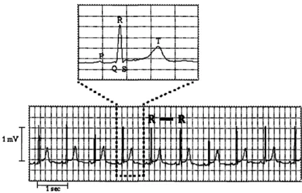
To precisely calculate the interbeat interval time series used in HRV analysis, we utilize the electrocardiogram (ECG), a record of the net electrical activity of cardiac cells. The synchronized depolarization and repolarization of atrial and ventricular cells trace out well-defined waveforms illustrated in the ECG in Figure 2-1. The "P" wave reflects atrial depolarization, the "QRS" complex corresponds to the electrical activation of the ventricles, and the "T" wave reflects ventricular repolarization

(re-ImVI

...-...-.. 4....-. .. _{' II}--- 4 - .... ...

I I

L.LI.I!.IJ.L. LI 9III L I~III.L1W.LL..4

-T " - %i-. ... ---.. ...." ; ---- ---... ..-... i ' .. --i i -.. ". i U T , i '-i ' '.'

- ii liii

iiri i i i-i i i i i rii ii it.

.•.. ,T,, T.!..I I ., ...-....: "-t I.. .- 1 . ,I ..... .,... .. .. .... ... ..,; , i.:... ,. ,

I- i I I tItIItI- I I-I-f I/lif ti-Il II I II Ii It I I I .-i 4I

i i"

.__.

Figure 2-1: Electrocardiogram record of cardiac electrical activity.

covery). From the ECG, we determine the cardiac interbeat interval by calculating the time between two consecutive "R" waves (R-R interval). While the "R" wave does not precisely represent the "onset" of the mechanical heart beat, it is chosen to measure the period between beats because it is less affected by measurement and quantization noise and is more readily identifiable [2]. We obtain the overall heart rate time series by calculating successive cardiac interbeat intervals. The ECG is often recorded from an ambulatory device known as a Holter monitor, which stores and digitizes the data. Ectopic beats, which do not originate in the SA node, are usu-ally removed before HRV analysis. These abnormal beats may occur even in healthy hearts, and often dominate the analysis if not excluded.

Autonomic Control of the Heart Rate

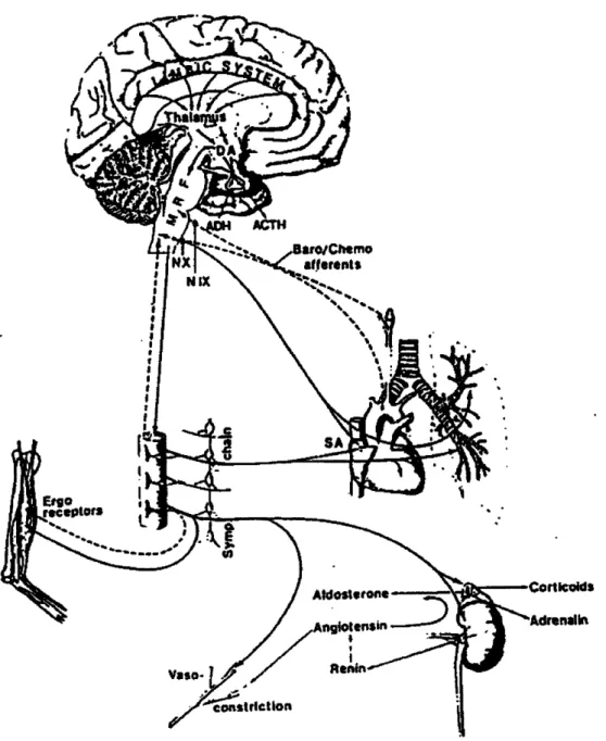
The firing activity of the SA node is strongly regulated by autonomic influences from the brainstem, mechanics of respiration and circulation, and circulating neuro-hormones [8]. This complicated feedback control system is schematized in Figure 2-2. Although local factors such as tissue stretch and temperature changes affect the discharge frequency of the SA node, the two branches of the autonomic nervous sys-tem (ANS) are the most important factors in determining the heart rhythm. These

I '

-•. ! T!I I• !.n-•' !'•' ! .•M•..r! w-l .n-•.- -I r i-! TT•I t

__i__i_.1. J L i 1....[ .~_ i..1.i _ _i._.i. . J.1 . ,_l).l _;_ J_,_ . 1.__i__i 1.i.i.1.i. _i i j.l__i__ .. 1. . .l.ll.i .i.i .-- i il --i-i i-.. i.. ,

Is

.. .i*

I

I I1 iI

two branches, the parasympathetic (vagal) and sympathetic system, are regulated by higher centers located in the brain. Cardiac parasympathetic fibers originate in the dorsal motor nucleus (medulla oblongata), while sympathetic fibers originate in the vasomotor center [8]. Both the parasympathetic and the sympathetic system innervate the sino-atrial node, and thus the net effect of these systems impact the overall heart rate. The effects of these systems are mediated through neurotransmit-ters (norepinephrine in sympathetic, acetylcholine in vagal), which alter the electrical activity of pacemaker cells. Specifically, parasympathetic stimulation decreases the firing rate of the pacemaker cells, while sympathetic stimulation increases the firing rate.

Alterations in heart rate can be evoked by changes in blood pressure [3]. Trans-ducers known as baroreceptors located in the aortic arch and carotid sinuses send feedback to the central nervous system. A change in blood pressure will elicit a change in heart rate through reciprocal changes in activity in the two autonomic divisions. The heart rate is also significantly affected by mechanical aspects of circulation, pri-marily respiration. Specifically, during inspiration, the heart rate increases, while in expiration, the heart rate decreases. This coupling of the heart rate to respiration is known as "respiratory sinus arrhythmia." It is important to note that this variability is indicative of a healthy condition, not a diseased one [2]. In addition, the cardio-vascular system is connected to many relatively independent resistances within the circulation network. By varying its resistance, each tissue regulates its own blood flow and pressures. The cardiovascular system is regulated by these individual resistances

[8].

The central nervous system acts by integrating information from various sensors within the cardiovascular system and controlling the rate of the heart beat through the peripheral ANS. Recently, there has been interest in studying HRV to gain insight into the nonlinear competition between sympathetic and parasympathetic mechanisms that govern the cardiovascular system [9]. A direct measurement of the parasympa-thetic and sympaparasympa-thetic activity is not clinically feasible; HRV, while indirect, provides a non-invasive indicator of integrated neuroautonomic control. The complex control

Figure 2-2: Complex feedback systems operating over wide range of temporal and spatial scales that regulate the dynamics of the heart rate. ADH - Antidiuretic hormone; ACTH - Adrenocorticotrophic hormone; SA - sino-atrial node.

feedback system of the cardiovascular system is not fully understood. However, both nonlinear and linear analysis of HRV have considerably advanced our current under-standing of this system.

2.1.1

Linear Methods of Assessing Heart Rate Variability

(HRV)

The beat-to-beat variability of the heart can be considered the integrated regulatory response of the cardiovascular system to intrinsic and extrinsic perturbations [1]. Ex-amples of these perturbations range from changes in posture to adjustments in local vascular resistance in different tissue beds. A classical interpretation applied to a wide variety of physiologic systems is that the cardiovascular system acts in response to these disturbances to maintain homeostasis and achieve a physiological steady state [10]. According to this theory, developed by Walter B. Cannon of Harvard Medical School, we expect the heart rate to be relatively constant until perturbed and to remain at a constant value until perturbed again. This traditional homeostatic view-point assumes that the cardiovascular system under analysis is "well-behaved" and relatively "linear" - a change in the input elicits a proportional change in the output.1

The assumption of the heart rate as linear is widespread, and many techniques have utilized this principle for both clinical application and physiologic understanding of the cardiovascular system.

Traditional statistics to quantify HRV include the mean and the standard devi-ation (first and second moments). These straightforward measures provide useful clinical application. For example, CHF is often associated with a decreased vari-ability, as measured by standard deviation, compared to normal heart rate dynamics [11]. This characteristic is evident in the interbeat interval time series of a CHF patient shown in Figure 2-3 part (b), as contrasted to the heart rate time series of a healthy patient, shown in part (a). In addition, several studies have demonstrated that a lower standard deviation is associated with an increased mortality after

1.0 0.8 0.5 0.4 0 1.a 0.5 04A .o 500.0 1000.0 500aa.0 2000.0 Beat Number

Figure 2-3: Heart rate time series for (a) healthy subject and (b) patient with conges-tive heart failure (CHF). Note the higher mean resting heart rate (lower R-R interval) and reduced variance in CHF.

ocardial infarcation. Thus, traditional HRV analysis plays an important prognostic role, especially because the patient can be monitored non-invasively.

Because the mean and standard deviation yield limited insight into the beat-to-beat dynamics of the heart rate, linear analysis is frequently applied. In a linear pro-cess, all frequency components are uncorrelated; thus, Fourier phases are randomized. Linear analysis, e.g. power spectral analysis, is traditionally used to characterize such processes. This technique uses Fourier methods to decompose a process into a super-position of sinusoids with different amplitudes and frequencies. The power spectrum presents the squared amplitude of these sinusoids as a function of frequencies. With this technique, oscillations present in the heart rate can be identified and correlated with physiological phenomena [2]. For example, the healthy heart rhythm, which is modulated by respiratory activity, oscillates with a frequency of approximately .25 Hz

(corresponding to one respiratory cycle every four seconds). An oscillation may also be apparent at approximately .1 Hz. While the origin of this 10 second oscillation is not fully understood, it is known that it is importantly influenced by the baroreflex. Studies have shown that fluctuations in heart rate that occur at frequencies greater than approximately .15 Hz are mediated by parasympathetic activity, while lower

frequencies are jointly mediated by the sympathetic and parasympathetic nervous system.

The presence or absence of an oscillation (a peak in the frequency domain) can indicate altered autonomic nervous activity, thus providing clinical information. For example, diabetes, a disease accompanied by dysfunction of the ANS, is associated with a decrease in respiratory sinus arrhythmia, as well as changes in the 10 second oscillation induced by body posture changes. In addition, the heart rate of some CHF patients contains a one cycle per minute oscillation. This pathologic pattern, associ-ated with Cheyne-Stokes breathing, will be discussed in more detail in Chapter 5.

It is important to recognize the clinical as well as physiologic importance of linear analysis indeed, certain aspects of heart rate control can be deduced without dealing with the nonlinearities inherent in the cardiovascular system. However, the complex dynamic nature of the beat-to-beat interval cannot be fully explained with conventional linear methods. Furthermore, the constancy predicted by homeostasis cannot account for the dynamic, apparently far-from-equilibrium behavior observed in "regular" sinus rhythm: the intrinsic, highly irregular variability of the normal heart rate does not seem to correspond to a steady state [10]. In recent years, the assumption of HRV as a linear process has been challenged by increased evidence that many complex nonlinear interactions exist in physiologic systems, including the cardiovascular system. Consequently, researchers employ nonlinear analysis to more fully explain complex cardiac dynamics [5].

2.1.2

Nonlinear Methods of Assessing HRV

Nonlinear dynamics are used to study systems that respond disproportionately to stimuli [12]. Such a system cannot simply be dissected into its components, since the modes of the system interact. As a result, a nonlinear mechanism can produce a highly complex output, such as the heart rate. In addition, in nonlinear systems, small changes in a control parameter can lead to large changes in behavior. A wide class of different behaviors can typically result from even a simple nonlinear process. A typical feature of heart activity is the heterogeneous, intermittent patterns that

change with time.2 When nonlinear dynamics are used to characterize HRV, these sudden dramatic changes in cardiac behavior do not need to be attributed to an equally dramatic change in cardiovascular control.

Chaos is a branch of deterministic nonlinear dynamics that has been applied recently to quantify and explain erratic cardiac behavior [5]. The term "determinis-tic" implies that chaotic systems are not strictly random, but rather the equations, parameters, and initial conditions are known and can be completely described math-ematically. A chaotic process demonstrates aperiodic dynamics and demonstrates a sensitive dependence on the initial conditions: a minor change in the initial condi-tions may cause a marked difference in the outcome (known as the "butterfly effect"). Nonlinear chaos is not characterized by a complete state of disorganization as the ver-nacular suggests, but rather a constrained type of randomness which is associated with fractals - the geometric concept of scale-invariance or self-similarity which applies to the structure of chaotic (strange) attractors.

The properties of heart rate time series as well as the underlying physiology con-trolling the cardiovascular system demonstrate the possibility of chaotic or fractal influences in cardiac behavior [12]. Careful inspection of the heart rate reveals similar fluctuations on multiple different orders of temporal magnitude. Figure 2-4 demon-strates this scale-invariant characteristic, which is absent in any non-fractal process. Self-similar processes are found in a range of physical systems ranging from earth-quakes to other biological systems. These processes are characterized by a power spectrum with a "1/f" power law decay that contains the same spectral power in any decade of frequency. Figure 2-5 displays this 1/f power spectrum of a healthy heart rate time series analyzed over several hours. This scale-invariant "fractal" manner of the heart rate is consistent with, but not diagnostic of chaos, since fractals may also arise from stochastic mechanisms.

The broad spectrum of the heart containing superimposed peaks in frequency (from the baroreceptor reflex and respiration) is also consistent with (but not neces-sarily indicative of) chaos [12]. In addition, phase space trajectories of the heart rate

2

CO a, a) 0) .0 2) C 29000 30000 31000 32000 33000 34000 35000 Beat Number

Figure 2-4: Self-similarity property of the fractal-like heart rate.

l0 10, 105 10, 10-' 0.000 0.001 0.010 Frequency (Hz) 0.100

reveal a complicated "attractor," rather than a periodic or fixed-point attractor seen in linear or regular processes.

What are the physiological mechanisms which induce this complex HRV? Heart rate control is influenced by the interaction of several central nervous system oscilla-tors and control loops. The interaction of these physiologic control systems operating on different time scales may induce irregular time courses that create scale-invariance in the heart rate [9]. Additionally, the feedback loops present in the heart produce de-lays in response time. Glass and Mackey [12] have emphasized the importance of time delays in chaotic systems. Another proposed mechanism which causes complex be-havior in HRV arises from competing neuroautonomic inputs of the parasympathetic and sympathetic branches of the nervous system.

The highly variable nature of the heart rate supports several functional purposes [10]. First, the erratic fluctuations in the healthy heart rate serve as an important mechanism for creating adaptability, or the ability to respond to unpredictable and changing perturbations. In addition, the absence of a characteristic time scale creates a broad frequency response that prevents the system from becoming mode-locked (locked to a single frequency). Finally, the long-range (fractal) correlations found in healthy patients indicate an overall principle for structuring highly complex nonlinear processes that generate fluctuations over a wide range of time scales [9].

Not surprisingly, a number of pathologies are characterized by a breakdown of the complex nonlinear dynamics observed in healthy heart function [6]. This breakdown may be manifest by a loss of complex variability, sometimes with the emergence of highly periodic behavior. For example, spectral analysis of ECG waveforms associated with sudden cardiac death reveals a narrow spectrum, rather than a broad spectrum apparent in chaotic systems. In addition, patients with severe left ventricular failure typically display two patterns: a strong, low frequency oscillation in heart rate (.01-.06 Hz) and reduced beat-to-beat variability. Similar pathologic patterns have also been observed in fetal distress syndrome. In general, emerging regularities indicate a decreased nonlinear complexity in pathologic patients,

demon-strating deterministic chaos. Two such measures used to quantify phase-space plots are the correlation dimension (CD), a measure of the complexity of the process, and the Lyapunov exponent (LE), a measure of the predictability of the process [13]. These measures have been applied to cardiac behavior with conflicting results [14]. The reliability of these methods is questionable, since these methods have difficulty distinguishing deterministic chaos from linear correlated stochastic processes [6]. In general, characterizing a process as "chaotic" with complete certainty is a difficult task.

Previous application of chaos-related metrics demonstrates the potential useful-ness of using dynamic nonlinear analysis to understand the complexities of the car-diovascular system. However, chaos is a sub-topic of the field of nonlinear dynamics, specifically applicable only to deterministic systems. It is unlikely that the cardiovas-cular system is purely deterministic since stochastic influences are likely to affect the overall state of the system. While the methods of CD and LE inherently assume that the system is "chaotic," other methods of statistical analysis have investigated more general nonlinearities in HRV. For example, Ivanov et al. [4] have used wavelet-based time series analysis to elucidate the nonlinear phase interactions between the different frequency components of the beat-to-beat interval.

In nonlinear systems (deterministic and stochastic), the Fourier phases of the signal interact in a non-random fashion. Thus, the harmonic components are not statistically uncorrelated. This Fourier phase dependence, a defining feature of the nonlinearity present, cannot be addressed with linear techniques. A technique that has previously been used to describe nonlinear interactions between Fourier phases is called higher order spectral analysis (HOSA). Although HOSA has been applied to a variety of physical systems, its application to HRV is relatively uncharted. By applying HOSA to the heart rate, the nonlinearly induced phase-couplings can be investigated, potentially improving our understanding of the complex processes of the ANS.

2.2

Higher Order Spectral Analysis (HOSA)

Since their first application in 1963, higher order statistics have been used to analyze a range of complex systems including telecommunications, sonar, radar, plasma physics, economic series, and biomedicine [15, 16, 17]. These statistics, known as cumulants, and their associated Fourier transforms, known as higher order spectra, extend beyond the second order characteristics of a signal to extract phase information as well as information due to deviations from Gaussianity. For general signal analysis purposes, there are two main motivations for using HOSA [17]:

1) To detect and quantify nonlinear interactions between Fourier components of a time series.

2) To suppress Gaussian noise processes for detection and classification problems.

Before we can explore these applications of HOSA, we must first introduce more rig-orous definitions of linearity and nonlinearity, as well as the definitions of cumulants.

2.2.1

Gaussian Processes

By definition, a Gaussian, or "linear", process is fully described by its first order characteristics (i.e. the mean) and second order characteristics (i.e. the autocorrela-tion or power spectrum). The autocorrelaautocorrela-tion, C2.(T) (also known as the two-point

cumulant), of a process x(k) of finite length N, is defined as:

1 N-7 1 2

N

x(k)=1

(k

_(2.1)k=1

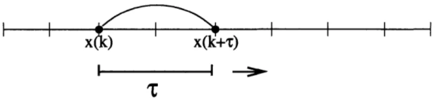
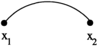
where (-) denotes the expected value operation. For finite length stationary, ergodic processes3, we approximate the ensemble expected value as a time average operation. This operation can be visualized as the process in Figure 2-6. For a set time lag, T,

3

A process, x(k) is ergodic if all its moments can be determined from a single observation. This implies that all time averages of all possible sample realizations equals the ensemble average [16, 17]. In addition, stationarity implies that the statistics of y(k) do not change with time. In our analysis, we will assume all processes are ergodic.

x~k) X(k--)

Figure 2-6: Autocorrelation for x(k).

we multiply x(k) with x(k + T) (represented as the arc), and average this value for all k (sliding the connected points along the axis). To gain a physical intuition of autocorrelation, consider flipping an unbiased two-sided coin. Each point on the x axis, k, corresponds to one flip of the coin. A flip resulting in a head corresponds to a value of 1, whereas a tail corresponds to a value of -1. Because there is an equal probability of producing a 1 and a -1 (a head or a tail), the average of all products x(k)-x(k+7) will be zero. Thus, for any time lag 7 -4 0, there is no correlation between x(k) and x(k + r): knowledge of the present value of x(k) provides no information for a future value at x(k + T).

Now, consider the following recursively defined equation:

x(k + 1) = ax(k) + w(k) (2.2)

where w(k) is a stationary white Gaussian noise sequence. For a given T, the value of x(k + T) depends on a previous value x(k) by definition of recursion. Thus, this relationship between two points, called the autocorrelation, completely describes the process defined by Equation 2.2. More generally, the autocorrelation is sufficient for describing any zero-mean Gaussian process. Consequently, for such processes, all higher order moments provide no additional information because they can be ex-pressed in terms of second order characteristics. For a set of zero mean (jointly) Gaussian random variables, {Xl, X2, ... XL}, with autocorrelation4 y, higher order

ments can be decomposed as follows [18]:

(XlX2X3 ... XL) = L odd (2.3)

E Yjlj2'Yj 3i4'jL-1jL L even

where the summation is over all distinct pairings {jlj2}, ... {jL-jL} Of the set of

integers 1, 2, ...L.

Alternatively, the power spectrum, which is the Fourier transform of the autocor-relation, is an equivalent second-order characteristic which also completely describes a Gaussian process. Formally, the power spectrum, S2x(f), is defined for a process x(k) with corresponding Fourier transform X(f) as5

S2x(f) = X(f)X*(f) =

IX(f)1

This classical method evaluates the power of each frequency component, suppressing all phase information [17]. An important characteristic of Gaussian processes is that all frequency components are uncorrelated, i.e., Fourier phases do not interact and are random. It therefore follows that phase-blind statistics completely describe Gaussian processes since they have randomized phases.

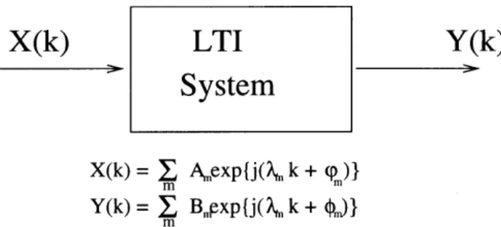
Because Gaussianity is preserved under linear operations, all linear systems with Gaussian inputs generate Gaussian (randomized phase) outputs. For example, Fig-ure 2-7 shows several sinusoids with varying amplitudes, phases, and frequencies as the input, X(k), to a linear time-invariant (LTI) system. Due to linearity, the out-put, Y(k), consists of the superposition of these sinusoids with the same frequency components scaled and shifted. However, because Fourier components of X(k) are uncorrelated, no coupling occurs between phases, 0,, of the sinusoids Y(k) [17].

5

X(k)

Y(k)

X(k) = , Amexp{j(k k + pm)}

Y(k)= 1 Bmexp{j(k k+ 0)}

m

Figure 2-7: Linear time invariant (LTI) system with sinusoidal inputs, and uncorre-lated harmonic components at the output.

X(k) = 1 Aexp{j(•, k +(PI)}

Z(k) = E I CmC.exp{j(Xm+ X.n)k + (qm+ cn)}

Figure 2-8: An example of a nonlinear (NL) quadratic system with sinusoidal inputs, and correlated harmonic components at the output.

2.2.2

Nonlinear Processes

In a nonlinear process, a (frequently complex) interaction exists between Fourier phases of a time series. Consider the quadratic nonlinear system shown in Figure 2-8. This system clearly induces phase coupling at the output Z(k) [17]. To examine such a process (i.e., nonrandom phase), we cannot rely on classical linear methods. Rather, we turn to a more sophisticated method - higher order statistics. We begin our study of HOSA by introducing the third order cumulant, a higher order statistical technique for examining nonlinear processes.

For random variables xl, x2, and x3, the third order cumulant is defined as:

CUm(xI, x2, 3) (X31 2X3) - (Xl)(X2X3) - (X2) (X21 3)

--(X3)(X1 2) + 2(x 1)(X2)(X3) (2.5)

LTI

System

Given a strictly stationary, random process x(k), the third order cumulant of x(k), denoted as c3x(71, r2), is given by [17]:

c

(71-,

7

)

=

cum

{f(k)Z(k

+ Ti)x(k

+

T

)

= (x(k)x(k + T1)x(k + T2)) - (x(k)){(x(k)x(k + Ti)) + (x(k)x(k + T2))

+(x(k + T1)x(k + 72))} + 2(x(k))3 _(2.6)

obtained by substituting xl = x(k), x2 = x(k + Ti), and x3 = x(k + T2) into

Equa-tion 2.5 and noting that (x(k)) = (x(k + T1)) = (x(k + 72) = mx by stationarity. Defining the moment function as

mnx(71, T2, .. Tn- 1) -- (x(k)x(k + T1)...x(k + Tn-1)) (2.7)

we can rewrite Equation 2.6 as

C3x(T1, T₂) = m3x(T1, T2) - (mx(m2x(T1) + m2x(T1) + 2x (T2 - 71)) - 2m

3_{) (2.8)}

Additionally, the third order cumulant can alternatively be written as:

C3x(T1, T2) = m3 (T1, T2) - mG (T1, T2)

(2.9)

where m3x(71, •2) is the third order moment function of x(k) and m G(71, 2) is the

third order moment function of a Gaussian random process with the same first and second order characteristics as x(k) (which we will denote as xG(k)). We derive this result by first observing that all odd moments of a zero mean Gaussian random process are zero (from Equation 2.3). To obtain zero mean random processes, denoted by G (k), ýG (k + Ti), G (k + T2), we must subtract the mean from each process:

AG(k) = ZG(k) - m (2.10)

G

(k + 1)

=

(k +

- mx

(2.11)

Hence,

(jG(k)>G(k + T1)G(k + T2)) = 0 (2.13)

Substituting Equations 2.10 through 2.12 into Equation 2.13, we obtain

((xG(k) - mx)(xG(k + T) - mx)(xG(k + 72) - mx)) = 0 (2.14)

Multiplying all terms, and after some algebra we obtain:

m3G(71, 2)

=

(xG(k)ZG(k+Tl)XG(k+T

))=

m•(-m2

71

)M7 272)+m2X(72 -))-2

(2.15)

This decomposition process can be visualized with Figure 2-9 (with the arc represent-ing the moment operation, and the blue circle representrepresent-ing the mean). An important result of Equation 2.9 is that for a (randomized phase) Gaussian process, x(k), the third order cumulant is zero [17]:

m3x (71, 72) = mG (71,72) SC3,(7T1,72) = 0

In addition, we note that for zero mean processes, the third order cumulant and the third order moment operation are equivalent, thus Equation 2.9 simplifies to

cU (TI,

72)

x

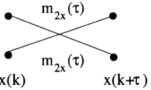
Whereas the autocorrelation examines the relationship between two points, the third-order cumulant examines the relationship between combinations of three points within a time series (Figure 2-9), removing Gaussianities. By only preserving non-randomized phase information, the third-order cumulant captures nonlinearities.6

3x (

,2 )

m3x (

,'2

)

m (

2

Gaussian Process:

3x (T 1J

)

+

-2

Nonlinear Process:

m

_{x ( 1}

_'2

₎

Figure 2-9: C3.(T1, 2) for a process x(k).

...

..

.

...

....

..

...

.

-I-. .. . i

2.2.3

Quadratic Phase Coupling Example

To further demonstrate why second order characteristics are insufficient for describing nonlinearly induced phase coupling, consider the time series given by

s(t) = cos(wit + 01) + cos(w2t + 82) + cos(w3t + 93) (2.17)

where

w3 = w1 + w2 (2.18)

and 01, 02 are randomly distributed in [0, 27). Consider two cases:

Case 1: 03 randomly distributed in [0, 27r)

Case 2: 03 = 01 + 02.

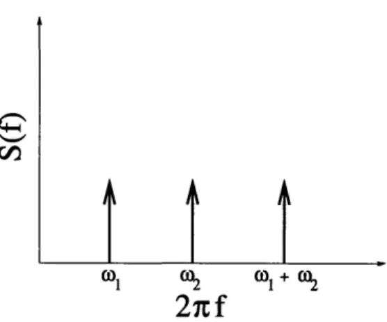
If 03 is independent of 01, 02 (case 1), then a time series consisting of many realizations of s(t) with different sets of random phases will have Gaussian statistics. However, in case 2, the phases 01 and 02 of s(t) are "completely" coupled. This phenomenon, known as quadratic phase coupling (QPC) [15], results from a quadratic nonlinear system which induces interaction between Fourier components (causing contributions to the power at sum and/or difference frequencies). The power spectrum of s(t), shown in Figure 2-10, conceals phase relations of harmonic components, and therefore fails to discriminate case 1 from case 2. For cases 1 and 2, the third order cumulants can be easily obtained [17]. For case 1,

c3s(T1, T2) 0 (2.19)

However, for case 2:

1

C3s (T, T₂) = -COS(W₄ 2T1 + WlT2) + COS(W3T1 - WT12) +

cos(wiT1

+

W

7

)

+

COS(W371

-

W

T

)

+

t t'

(0 1 0 + 0h

2if

Figure 2-10: Power spectrum, S2x(f), for s(t) with both randomized phases (case 1)

and quadratic phase coupling (case 2).

To see this result more intuitively, we turn to the frequency domain and introduce the auto-bispectrum, which is formally defined as the Fourier transform of the third-order cumulant:

1 00 00

Sa(1, f)=

J

S3U(f1, f2) = (X(fi)X(f2)X*(fi + f2)) (2.22)

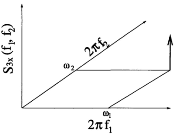
From Equation 2.22, we can see that if the Fourier components are uncorrelated (as in case 1), the average triple product of the Fourier components is zero, producing a zero bispectrum. However, in case 2, the coupling of the Fourier components results in a nonzero bispectrum with a peak at (fi, f2), indicating the oscillation at fi + f2 results from a nonlinear interaction between fi and f2. This result, shown in Figure 2-11, demonstrates the utility of HOSA for detecting quadratic phase coupling in signals.

2.2.4

Conclusion

HOSA has previously been applied to a variety of systems. Specifically, these systems contain "quadratic" nonlinearities, which induce phase coupling between triads of

co1

21 f,

Figure 2-11: Bispectrum displaying peak at (wi, w2) due to phase coupling between

wl and w2.

Fourier modes (such as discussed in the QPC example) [15]. By applying bispectral analysis, the cross-spectral transfer of energy resulting from these nonlinearities can be detected and quantified. While HOSA has been applied in previous works to study frequency interactions, these interactions are usually quite simple, involving a phase coupling between only two or three frequencies. However, in many nonlinear processes, such as those with 1/f power spectra, more complex nonlinear frequency interactions exist. Because of these complex frequency relationships, performing the higher order analysis in the time domain will be just as informative as the frequency domain'. Before applying HOSA to highly complex heart rate time series, we begin by applying HOSA to well described processes with calculable third-order cumulants to gain further understanding of the uses and potential limitations of this method.

7

Generally, higher order spectra rather than cumulants are computed to analyze nonlinearities.

4-4

Cn1

Chapter 3

Basic Investigation of HOSA:

Mathematical Modeling

To better understand the use of cumulants for the study of nonlinear "real world" systems, we first apply higher order cumulants to fully characterized mathematical models. By applying higher order cumulants to well-known nonlinear processes, we can address several key questions. Specifically, we can examine finite-size effects, nonstationarity effects, and unexpected numerical problems that may arise in com-putation. Furthermore, we can assess the effectiveness of HOSA for both detecting and quantifying general nonlinearities, and determine the sensitivity of the third order cumulant to power-law nonlinear frequency interactions.

3.1

Computation of

c3(71,

for Gaussian

Ran-dom Processes Applied to a Nonlinear

Sys-tem

To explore HOSA and its limitations, it is most informative to examine nonlinear processes, y(k), arising from the most general nonlinear systems:

Brillinger [17] suggests that many nonlinear relationships may be approximated by the system:

y(k) = x(k) + xz"-l(k) (3.1)

for different orders n. For n = 2, the system is linear (y(k) = (1 + 3)x(k)). However, n = 3 corresponds to the quadratic nonlinear system we will use in our analysis:

y(k) = x(k) + px2_{(k) (3.2)}

This quadratic nonlinear system, while simple, describes a wide variety of physical systems.

The input to this quadratic nonlinear system will be a zero-mean, stationary Gaus-sian random process x(k) described by its autocorrelation, C2x(T). From Section 2.2, we recall that higher (third and fourth) order cumulants of a Gaussian random pro-cess are zero. However, when this propro-cess serves as the input to a nonlinear system, the output is a non-Gaussian random process with non-zero higher order cumulants. In this chapter, we compute the third order cumulant of y(k) for two different inputs x(k). One of these inputs is characterized by an exponentially decaying autocorrela-tion, the other by long-term correlations.

For any Gaussian input, x(k), the third order cumulant of y(k) (described by Equation 3.2), c₃y(1i, T2), can be expressed as a combination of higher order moments

of x(k). In addition, because x(k) is Gaussian, all higher order moments of x(k) can be decomposed into a combination of first and second order moments as described in Equation 2.3. Because the first moment (the mean) of x(k) is zero, c3y(T1, T2) can be written explicitly in terms of only the second order characteristics of x(k), m2x(T). It is important to note that this relationship is independent of the choice of m2(T).2

From Equation 2.1, and from the fact that x(k) is zero mean, we note that the second order moment of x(k), m2x(T), defined as:

is equivalent to c2x(7,). Thus, we will use m2x((7) (rather than c2x( T)) to denote the

autocorrelation of a zero mean random process. By definition, the third order cumulant of y(k) is:

C3y(T1 , T2) = (y(k)y(k + TI)y(k + T2)) - (y(k)){(y(k)y(k + Ti)) + (y(k)y(k + 72)) +

(y(k + Ti)y(k + T72))} + 2(y(k))3 (3.4)

- m3y (T1,7 ₂) - my (m2y(T1) m2y(T2) + m2y(T2 - T1)) + 2m3 (3.5)

To determine c3y (TI, 72), we must first obtain my, m2y(T), and m3y(71, T2). We begin

by finding my and m2y(7), the first and second moments of y(k). Using Equation 3.2

and the fact that (x(k)) = 0, we have

MY

(x(k)

Furthermore, we expand the terms in Equation 3.7. Because x(k) is Gaussian, (from Equation 2.3) we eliminate all odd order moments. Thus, we have

m

=

(x(k)x(k

))

+

3

(

_(k)X

_(k

₊

₎₎

= m2x (7)+ O 2(k)x 2(k + T)) (3.8)

To decompose the fourth order moment (x2_(k)x 2_{(k + 7)), we consider all possible}

combinations of second order moments. We graphically represent the second order moment (xlx2) as shown in Figure 3-1. For any given combination, we multiply all

second order moments together. Finally, we sum the products from all combinations. It is helpful to visualize this decomposition process.

X₁

X2

Figure 3-1: Depiction of second order moment, (xlx2).

m2x (0)I m 2x(0)

x(k) x(k+r)

Figure 3-2: Combination 1 for fourth order moment (x2_(k)x2_{(k + T)).}

To facilitate this decomposition, we consider each combination separately. One possible combination of the points x(k), x(k), x(k + T) and x(k + T) is shown in Figure 3-2. The product of the second order moments within this combination is

m2x(0). Next, we consider the combination shown in Figure 3-3. This combination yields the product m2x(T). Likewise, the same product results from the combination in Figure 3-4. Summing these combinations, we obtain

(2

(k)x

_{(k +}

_T))

₌

_m,

_(O)

_{+ 2mx (7)}

_(3.9)

m₂x(r)

x(k) m2x

x(k+c)

m2x ()

x(k) x(k+t)

Figure 3-4: Combination 3 for fourth order moment (x2(k)z 2_{(k + 7)).}

We can now determine the second order moment:

m21(T) = m2x(T) +

2

m2X(0)

+

(3.10)

The next step in calculating C3x (T1, ₂) is to determine m3y (Tl, T₂)

mT3y(TI,7 2) = ((x(k) + 3xZ2(k)) (x(k + 7T) + /x 2(k + 7T)) (x(k + T2)+ +x2(k + T2)))

(3.11)

After expanding terms in Equation 3.11, all odd moments are again removed. All even moment terms are collected, and can further be broken down into a superposition of second order moments.

m3y(71, 72) = (3x(k)x(k + T)X 2 (k + 2) + x(k) 2(k + (k )(k +T 2) +

Zx2(k)x(k + T1)x(k + T2) + 03

3_x2_(k)x 2_{(k + T1)}2_{(k + 7T}

2)) (3.12)

We determine each term separately:

p(x(k)x(k

+

(k +

))