A fully Bayesian approach to the parcel-based detection-estimation of brain activity in fMRI.

HAL Id: cea-00333624

https://hal-cea.archives-ouvertes.fr/cea-00333624

HAL is a multi-disciplinary open access archive for the deposit and dissemination of sci-entific research documents, whether they are pub-lished or not. The documents may come from

L’archive ouverte pluridisciplinaire HAL, est destinée au dépôt et à la diffusion de documents scientifiques de niveau recherche, publiés ou non, émanant des établissements d’enseignement et de

A fully Bayesian approach to the parcel-based

detection-estimation of brain activity in fMRI.

Salima Makni, Jérôme Idier, Thomas Vincent, Bertrand Thirion, Ghislaine

Dehaene-Lambertz, Philippe Ciuciu

To cite this version:

Salima Makni, Jérôme Idier, Thomas Vincent, Bertrand Thirion, Ghislaine Dehaene-Lambertz, et al.. A fully Bayesian approach to the parcel-based detection-estimation of brain activity in fMRI.. NeuroImage, Elsevier, 2008, 41 (3), pp.941-69. �10.1016/j.neuroimage.2008.02.017�. �cea-00333624�

A fully Bayesian approach to the parcel-based

detection-estimation of brain activity in fMRI

Salima Makni

_{, J´erˆome Idier}

_,

Thomas Vincent

_{,Bertrand Thirion}

_,

Ghislaine Dehaene-Lambertz

_{and Philippe Ciuciu}

∗

(FMRIB), University of Oxford, John Radcliffe Hospital, Oxford, UK.

b_{IRCCyN (CNRS), Nantes, France.} c_{CEA, NeuroSpin, Gif-sur-Yvette, France.}

d_{IFR 49, Institut d’Imagerie Neurofonctionnelle, Paris, France.} e_{INRIA Futurs, Orsay, France.}

f_{INSERM U562, NeuroSpin, Gif-sur-Yvette, France.}

Abstract

Within-subject analysis in fMRI essentially addresses two problems, i.e., the

de-tection of activated brain regions in response to an experimental task and the esti-mation of the underlying dynamics, also known as the characterisation of

Hemody-namic response function (HRF). So far, both issues have been treated sequentially while it is known that the HRF model has a dramatic impact on the localisation of activations and that the HRF shape may vary from one region to another. In this pa-per, we conciliate both issues in a region-based joint detection-estimation framework that we develop in the Bayesian formalism. Instead of considering function basis to account for spatial variability, spatially adaptive General Linear Models are built upon region-based non-parametric estimation of brain dynamics. Regions are first identified as functionally homogeneous parcels in the mask of the grey matter using a specific procedure (Thirion et al., 2006). Then, in each parcel, prior information is embedded to constrain this estimation. Detection is achieved by modelling acti-vating, deactivating and non-activating voxels through mixture models within each parcel. From the posterior distribution, we infer upon the model parameters using Markov Chain Monte Carlo (MCMC) techniques. Bayesian model comparison allows us to emphasize on artificial datasets first that inhomogeneous gamma-Gaussian mixture models outperform Gaussian mixtures in terms of sensitivity/specificity trade-off and second that it is worthwhile modelling serial correlation through an AR(1) noise process at low signal-to-noise (SNR) ratio. Our approach is then val-idated on an fMRI experiment that studies habituation to auditory sentence rep-etition. This phenomenon is clearly recovered as well as the hierarchical temporal

organisation of the superior temporal sulcus, which is directly derived from the parcel-based HRF estimates.

Key words: Bayesian modelling, fMRI, gamma-Gaussian mixture model,

detection-estimation, Markov Chain Monte Carlo methods, Bayes factor, model comparison.

1 Introduction

Since the first report of the BOLD effect in human (Ogawa et al., 1990), func-tional magnetic resonance imaging (fMRI) has represented a powerful tool to non-invasively study the relation between cognitive stimulus and the hemody-namic (BOLD) response. Within-subject analysis in fMRI is usually addressed using a hypothesis-driven approach that actually postulates a model for the HRF and enable voxelwise inference in the General Linear Model (GLM) framework. In this formulation, the modelling of the BOLD response i.e., the definition of the design matrix is crucial. In its simplest form, this ma-trix relies on a spatially invariant temporal model of the BOLD signal across the brain meaning that the expected response to each stimulus is modelled by a single regressor. Assuming the neurovascular system as linear and

time-invariant (LTI), this regressor is built as the convolution of a sparse spike train

representing the stimulation signal and the canonical HRF, i.e., a composition of two gamma functions which reflects the BOLD signal best in the visual and motor cortices (Glover, 1999).

Intra-individual differences in the characteristics of the HRF have been exhi--bited between cortical areas in (Aguirre et al., 1998; Miezin et al., 2000; Neumann and Lohmann, 2003; Handwerker et al., 2004). Although smaller than inter-individual fluctuations, this regional variability is large enough to be regarded with care. To account for these spatial fluctuations at the voxel level, one usually resorts to hemodynamic function basis. For instance, the canonical HRF can be supplemented with its first and second derivatives to model differences in time (Friston, 1998; Henson et al., 2002). To make the basis spatially adaptive, Woolrich et al. (2004a) have proposed a half-cosine parameterisation in combination to the selection of the best basis set. Al-though powerful and elegant, the price to be paid for such a flexible modelling lies in a loss of sensitivity of detection: the larger the number of regressors in the basis, the smaller the number of effective degrees of freedom in any sub-sequent statistical test. Crucially, in a GLM involving several regressors per

condition, the Student-t statistic can no longer be used to infer on differences between experimental conditions. Rather, an unsigned Fisher statistic has to be computed, making direct interpretation of activation maps more difficult. Indeed, the null hypothesis is actually rejected whenever any of the contrast components deviates from zero and not specifically when the difference of the response magnitudes is far from zero.

In this paper, to facilitate cognitive interpretations, we argue in favour of a spatially adaptive GLM in which a local estimation of the HRF is performed. This allows us to factorise the expected BOLD response with a single regres-sor attached to each experimental condition and to enforce direct statistical comparisons based on response magnitudes. However, to conduct the analysis in an efficient and reliable manner, local estimation is performed at the scale of several voxels.

As mentioned earlier, the localisation of brain activation strongly depends on the modelling of the brain response and thus of its estimation. Of course, the converse also holds: HRF estimation is only relevant in voxels that elicit signal fluctuations correlated with the paradigm. Hence, detection and estimation are intrinsically linked to each other. The key point is therefore to tackle the two problems in a common setting, i.e., to set up a formulation in which detection and estimation enter naturally and simultaneously. This setting cannot be the classical hypothesis testing framework. Indeed, the sequential procedure which first consists in estimating the HRF on a given dataset and then build-ing a specific GLM upon this estimate for detectbuild-ing activations in the same dataset, entails statistical problems in terms of sensitivity and specificity: the control of the false positive rate actually becomes hazardous due to the use of an erroneous number of degrees of freedom. We rather propose a Bayesian approach that provides an appropriate framework to address both detection and estimation issues in the same formalism.

The literature on Bayesian fMRI methods offers several approaches to ade-quately choose priors for detection. As introduced in (Everitt and Bullmore, 1999; Vaever Hartvig and Jensen, 2000; Penny and Friston, 2003) and further developed in (Smith et al., 2003; Woolrich et al., 2005; Ou and Golland, 2005; Woolrich and Behrens, 2006; Flandin and Penny, 2007), prior mixture models define an appropriate way to perform the classification or the segmentation of statistical parametric maps into activating, non-activating or deactivating brain regions. The pioneering contributions related to mixture modelling in fMRI (Everitt and Bullmore, 1999; Vaever Hartvig and Jensen, 2000) have proposed a voxel by voxel classification to decide whether the estimated effect is analogous to signal or noise in each voxel. Yet, the use of mixture mod-elling in a joint detection-estimation problem introduces specific concerns in comparison to the usual “hypothesis testing framework”. Indeed, our data are

required for the estimation step.

As regards HRF estimation, various priors may be thought of depending on the underlying HRF model. Basically, three classes of models coexist. Parametric models appeared first in the literature (Friston, 1994; Lange, 1997; Cohen, 1997; Rajapakse et al., 1998; Kruggel and Von Crammon, 1999). In this set-ting, the estimation problem consists in minimising some criterion with respect to (w.r.t.) some parameters of a precise function (e.g., Gaussian, gamma ,...). However, parametric models tend to introduce some bias in the HRF estimate, since it is unlikely that they capture the true shape variations of the brain dy-namics. Moreover, the objective function to be minimized is often non-convex making the parameter estimates unreliable and dependent of the initialisation. Hence, more flexible semi-parametric approaches have been proposed later to capture these variations (Genovese, 2000; G¨ossl et al., 2001; Woolrich et al., 2004a). In a semi-parametric framework, the HRF time course is decomposed into different periods (initial dip, attack, rise, decay, fall, ...), each of them being described by specific parameters. In the same time, non-parametric ap-proaches or Finite Impulse Response (FIR) models have emerged in the fMRI literature as a powerful tool to infer on the HRF shape (Nielsen et al., 1997; Goutte et al., 2000; Marrelec et al., 2003; Ciuciu et al., 2003; Marrelec et al., 2004). Most of these works take place in the Bayesian setting and constrain the HRF to be temporally smooth, which warrants a stable estimation in case of ill-posed identification.

Whatever the model in use, most methods are massively univariate and there-fore neglect the spatial structure of the BOLD signal. Early investigations have shown that estimating the HRF using regularised FIR models over a function-ally homogeneous region of interest provides more reliable results (G¨ossl et al., 2001; Ciuciu et al., 2004). In the following, a region-based non-parametric model of the HRF is therefore adopted. Then, the critical issue arising con-sists in exhibiting a functionally homogeneous clustering of the fMRI datasets over the whole brain. To that end, the grey matter’s mask is segregated into a few hundreds of connected Regions of Interest (ROIs), called parcels. The parcels are derived using the parcellation procedure proposed by Thirion et al. (2006), according to a compound criterion balancing spatial and functional ho-mogeneity. The second step of our analysis solves for the detection-estimation problem over each parcel.

The rest of this paper is organised as follows. Section 2 details how anatomical information is handled and how parcels are built up. Then, the forward parcel-based model of the BOLD signal is derived and priors over the unknown pa-rameters are specified. In Section 3, we explain the key steps of our inferential procedure based on MCMC methods, posterior mean (PM) HRF estimation and marginal Maximum A Posteriori (MAP) classification for detection. On artificial datasets, Section 4 reports the performance of our approach in terms

of sensitivity-specificity trade-off depending on the mixture prior and the noise modelling. In Section 5, our joint detection-estimation approach is tested on real fMRI data acquired during an habituation study to auditory sentence repetition. On the same datasets, we also performed a classical GLM analysis employing the widely used Statistical parametric mapping (SPM) software1_.

The two approaches are then compared and the main differences are exhib-ited. The pros and cons of the proposed method are discussed in Section 6 and some future extensions are envisaged.

2 Methodology

2.1 Definition of functionnally homogeneous brain regions 2.1.1 Anatomical representation

The segmentation of the grey-white matter interface is performed on an anatomical T1-weighted MRI image using the BrainVisa software2 (Mangin

et al., 1995). It provides us with the anatomical representation of the cortex. To accommodate the coarser spatial resolution of fMRI data (typically, 3.5mm along each direction), the grey matter mask Ma is dilated using a sphere as

structural element, with a radius equal to the resolution of functional images. Concurrently, a functional mask Mf was computed from the motion-corrected3

BOLD EPI volumes. Also, an average EPI volume was created. Then, we car-ried out a histogram analysis of this volume: a Gaussian density N (µ, σ2_{) was}

fitted on the main mode of the EPI signal of interest. A threshold defined as

µ − 3σ was used to obtain the functional mask. Finally, the mask of interest

where activation most likely occurs was built as Ms = Ma∩ Mf.

2.1.2 Parcellation of the grey-matter

The volume in mask Ms was then divided in K functionally homogeneous

parcels or ROIs using the parcellation technique proposed in (Thirion et al., 2006). The goal of this procedure is to segregate the brain into connected and functionally homogeneous components. For doing so, the parcellation algo-rithm relies on the minimisation of a compound criterion reflecting both the spatial and functional structures and hence the topology of the dataset. The spatial similarity measure favours the closeness in the Talairach coordinates

1 _{http://www.fil.ion.ucl.ac.uk/spm/} 2 _{http://brainvisa.info}

system. The functional part of this criterion is computed on parameters that characterise the functional properties of the voxels. These parameters can be chosen either as the fMRI time series themselves or as the β-parameters es-timated during a first-level SPM analysis. The latter choice is nothing but a projection onto a subspace of reduced dimension, i.e., the feature space. Typically, the feature space is defined from a F-contrast in a SPM analysis. The number of parcels K needs to be set by hand. The larger the number of parcels, the higher the degree of within-parcel homogeneity. Of course, there exists a trade-off between the within-parcel homogeneity and the signal-to-noise ratio (SNR). If the number of voxels is too small in a given parcel, the HRF estimation may become inaccurate, specifically in regions where no voxel elicits a specific response to any experimental condition. To objectively choose an adequate number of parcels, Thyreau et al. (2006) have used the Bayesian information criterion (BIC) and cross validation techniques on an fMRI study of ten subjects. They have shown converging evidence for K ≈ 500 for a whole brain analysis and recommend K = 200 as a fair setting for a restricted analysis to the grey matter’s mask leading to typical parcel sizes around a few hundreds voxels.

2.2 Parcel-based modelling of the BOLD signal

Vectors and matrices are displayed in lower and upper cases, respectively, both in bold font (e.g., y and P ). Unless stated otherwise, subscripts i, j, m and

n are respectively indexes over mixture components, voxels, stimulus types

and time points. We refer the reader to appendix A for the definitions of the non-standard probability density functions (pdf). Also, the pdf families are denoted using calligraphic letters (e.g., N and G for the Gaussian and gamma densities).

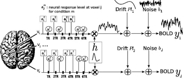
The regional forward model of the BOLD signal introduced in (Makni et al., 2005) is used to account for voxel-dependent and task-related fluctuations of the magnitudes of the BOLD response. Hereafter, the latter magnitudes are called Neural Response Levels (NRLs). In short, this time-invariant model characterises each and every parcel by a single HRF shape and a NRL for each voxel and stimulus type. As shown in Fig. 1, this means that although the HRF shape is assumed constant within a parcel, the magnitude of the activation can vary in space and across experimental conditions. Let P = (Vj)j=1:J be

the current parcel and Vj a voxel in P. Then, the generative BOLD model

reads: yj = M X m=1 am j Xmh + P `j+ bj, (1) where

• yj = (yj,tn)n=1:N denotes the BOLD fMRI time course measured in voxel Vj

at times (tn)n=1:N (N is the number of scans) with tn= nTR and TR is the

time of repetition,

• Xm _{= (x}m

tn−d∆t)n=1:N,d=0:D is a N × (D + 1) binary matrix corresponding

to the arrival times for the mth condition. ∆t is the sampling period of the HRF, usually smaller than TR. The onsets of the stimuli are put on the ∆t-sampled grid by moving them to the nearest time points on this grid. Note that Xm _{can be adapted to paradigms having trial varying stimulus}

magnitudes or durations.

• Vector h = (hd∆t)d=0:Drepresents the unknown HRF shape in parcel P (D+

1 is the number of HRF coefficients). It actually seems reasonable to assume a single HRF shape in homogeneous parcels.

• am

j stands for the NRL in voxel Vj for condition m (M is the number of

experimental conditions in the paradigm). Hence, the activation profile as-sociated to the mth stimulus type in voxel Vj is computed as the product

h × am

j .

• P = [p1, . . . , pQ] is the low frequency orthogonal matrix of size N × Q. It

consists of an orthonormal basis of functions pq = (pq(tn))n=1:N. To each

voxel is attached an unknown weighting vector `j that has to be regressed

in order to estimate the trend in Vj. We denote l = (`j)j=1:J the set of low

frequency drifts involved in P.

• bj ∈ RN is the noise vector in voxel Vj. In (Woolrich et al., 2001; Worsley

et al., 2002) an autoregressive (AR) noise model has been introduced to account for the serial correlation of the fMRI time series in the detection analysis. Importantly, when this temporal correlation is correctly estimated, the number of false positives decreases, yielding more conservative detection results. Similarly, in a joint detection-estimation framework, Makni et al. (2006b) have shown that the introduction of a spatially-varying first-order AR noise in model (1) provides a lower false positive rate. Hence, bj is

defined by bj,tn = ρjbj,tn−1+ εj,tn, ∀j, t, with εj ∼ N (0N, σ2εjIN), where 0N

is a null vector of length N, and IN is the identity matrix of size N.

Although the noise structure is correlated in space (Woolrich et al., 2004b) and non-stationary across tissues (Worsley et al., 2002), we do not essentially account for this correlation for two reasons. First, it is likely that a large part of the noise may be due to misspecification of the HRF. Second, we actually assume that the spatial correlation of the signal of interest is more important. Hence, the fMRI time series y = (yj)j=1:J are supposed to be

Fig. 1. Summary of the proposed regional BOLD model. The size of each parcel

P varies typically between by a few tens and a few hundreds: 80 6 J 6 350. The

number M of experimental conditions involved in the model usually varies from 1 to 5. In our example, M = 2, the NRLs (a1

j, a2j) corresponding to the first and the

second conditions are surrounded by circles and squares, respectively. Note that our model accounts for asynchronous paradigms in which the onsets do not necessarily match acquisition time points. As illustrated, the NRLs take different values from one voxel to another. The HRF h can be sampled at a period of 1s and estimated on a range of 20 to 25s (e.g., D = 25). Most often, the LFD coefficients `j are

estimated on a few components (Q = 4).

likelihood then factors over voxels:

p(y | h, a, l, θ0) = J Y j=1 p(yj| h, aj, `j, θ0,j) ∝ J Y j=1 |Λj|1/2σε−Nj exp µ − J X j=1 ˜ yt jΛjy˜j 2σ2 εj ¶ (2) where θ0,j = (ρj, σ2εj), θ0 = (θ0,j)j=1:J and ˜yj = yj− P mamj Xmh − P `j. Note that σ−2

εj Λj defines the inverse of the autocorrelation matrix of bj. According to

Kay (1988, Chap VI, p. 177), Λj is tridiagonal, with (Λj)1,1 = (Λj)N,N = 1,

(Λj)n,n = 1 + ρ2j and (Λj)n+1,n = (Λj)n,n+1 = −ρj ∀ n = 2 : N − 1. Its

determinant is given by |Λj| = 1−ρ2j. In what follows, we do not approximate

Eq. (2) by dropping the term |Λj|1/2, as done in previous works (Roberts and

Penny, 2002; Penny et al., 2003; Woolrich et al., 2004b). Indeed, when the AR parameter ρ significantly departs from zero (e.g., ρ ≥ 0.4), this approximation is biased and potentially far from the exact likelihood.

On the sole basis of the likelihood function (2), it seems impractical to identify the pair (h,_{a). Indeed, Maximum likelihood (ML) estimation of (h, a) is a} bilinear inverse problem since (1) is linear w.r.t. h when a is fixed and

vice-versa. Therefore, the ML solution (h∗_,a∗_{) is not unique. For instance, every}

the scale parameter s > 0. To get rid of identifiability problems and reach a more reliable estimation, in the Bayesian formalism we introduce suitable prior distributions attached to the unknown quantities (h,_a).

2.3 Priors

2.3.1 The Hemodynamic response function

Akin to (Buxton and Frank, 1997; Goutte et al., 2000; Marrelec et al., 2003), the HRF is characterised as follows: (i) its variations are smooth; (ii) it is causal and returns to a baseline after a given time interval T (ht= 0, ∀ t < 0

and t > T ); T is fixed by the user according to the experimental paradigm (usu-ally 25 seconds).

Condition (i) may be fulfilled using an approximation of the second-order derivative k∂2_hk2_:

(∂2h)dτ ≈ (h(d+1)τ − 2hdτ + h(d−1)τ)/τ2, ∀ d = 1 : D − 1.

In matrix form, we get ∂2_{h = D}

2h.

Condition (ii) is ensured with a HRF h whose magnitude vanishes at first and last time points (h0 = hD = 0). Hence, D2 is the truncated second-order

finite difference matrix of size (D − 1) × (D − 1) and k∂2_hk2 _{= h}t_R−1_{h with}

R = (Dt

2D2)−1 a symmetric positive definite matrix. The prior on h thus

reads h ∼ N (0, σ2

hR). To overcome the scale ambiguity problem mentioned

earlier, we constrain the HRF to be of unitary norm (khk = 1). Alternative constraints such as setting the value of the peak could be considered.

2.3.2 The “neural” response levels

Mixture models are often used as a second stage to segment the SPMs (i.e., the statistical maps) resulting from a first-level temporal analysis of fMRI time series (Vaever Hartvig and Jensen, 2000; Everitt and Bullmore, 1999; Woolrich et al., 2005). This means that the data to be classified correspond to some normalised effect ct_{β/ std (c}b t_{β), where vector c defines a contrast of}b

interest (typically a comparison between two experimental conditions) and βb

is the vector of parameter estimates after fitting a GLM against the fMRI data.

In the present paper, as well as in (Makni et al., 2005), prior mixture models are used in a different way, closer to that proposed by Svensen et al. (2000). In the same spirit, a mixture model is introduced on the NRLs for every ex-perimental condition m and not specifically on the linear combination ct_β.b

Table 1

Model definition and notations. Here, AR(1) stands for a first-order autoregres-sive noise in time whose parameters vary in space. In this respect, it is referenced as a varying AR(1) noise. The second noise model under study is a spatially-varying white noise. The columns describe the different NRLs priors: GMM stands for a two-class Gaussian mixture model (a zero-mean Gaussian density (G) for non-activating voxels and a Gaussian density (G) for non-activating voxels). GaGMM stands for a two-class gamma-Gaussian mixture model (a centred Gaussian density (G) for non-activating voxels and a gamma density (Ga) for activating voxels). GaGGaMM stands for a three-class mixture model composed of a zero-mean Gaussian density and two gamma densities (a gamma density (Ga) for activating voxels and a flipped gamma density (Ga) for deactivating voxels).

GaGMM GMM GaGGaMM AR(1) noise M1 M3

white noise M2 M4 M5

In (Makni et al., 2006a), it was stressed that a two-class Gaussian mixture model (GMM) may be inadequate for segregating noise from true activations. In particular, it can be shown that this kind of independent mixture may de-generate in the sense that the two probability density functions (pdf) overlap almost entirely if there are not enough activating voxels in the current par-cel (see (Makni et al., 2005, §VII.)). For this reason, we have rather adopted an inhomogeneous prior mixture model. Among several possibilities (Gaussian-lognormal MM, Gaussian-truncated Gaussian MM, ...), a gamma-Gaussian mixture model (GaGMM) has been retained for technical reasons that will become clearer in what follows. The non-activating voxels are still modelled using a zero-mean Gaussian pdf while a gamma distribution is used to enforce positivity of activating voxels. Akin to (Vaever Hartvig and Jensen, 2000; Woolrich et al., 2005), a three-class mixture prior model is actually considered to account for deactivating voxels. Since we assume that deactivation corre-sponds to a negative BOLD response, we use a flipped gamma density defined on the left part of the real line leading to define the GaGGaMM extension (see Table 1).

In our model, different stimulus types are supposed to induce statistically in-dependent hemodynamic magnitudes or NRLs i.e., p(a | θa) =Qmp(am| θm)

with a = (am₎

m=1:M, am = (amj )j=1:J and θa = {θ1, . . . , θm}. Vector θm

de-notes the set of unknown hyper-parameters related to the mth stimulus type. Because our mixture model is voxelwise, the prior pdf factors over voxels:

p(am_{| θ}m_{) =} Q

jp(amj | θm). Importantly, the hyper-parameters are kept

con-stant for all voxels in a given parcel because of the within-parcel homogeneity. These parameters may actually vary from one parcel to another. Let qm

j be

the allocation variable (the label) that indicates whether voxel Vj is activating

(qm

The marginal density p(am j | θm) thus reads: p(am j | θm) = 1 X i=−1 Pr(qm j = i | λm)f (amj | qmj = i, θm) = 1 X i=−1 λi,mfi(amj | θm), (3) with λm = (λ−1,m, λ0,m, λ1,m) and f0(ajm| θm) = N (0, v0,m), f±1(amj | θm) =

G(α±1,m, β±1,m). The λi,mparameters define the prior probabilities of the

three-class mixture on the NRLs (P_iλi,m = 1). For instance, λ1,m gives us the prior

probability of being activated in response to condition m. Since the mixture is independent in space, we have λ1,m = Pr(qjm = 1 | λm), ∀j. Note that qjm| λm

follows a multinomial distribution over the 3-dimensional probability simplex,

i.e., qm

j ∼ MN3(1; λm) (see Appendix A). Hence, seven hyper-parameters are

necessary to describe the prior mixture for each experimental condition m:

θm_{= {λ}

±1,m, α±1,m, β±1,m, v0,m}.

Compared to (Woolrich et al., 2005), we set the mean of the non-activating class to zero (µ0,m = 0, ∀ m), while we do not need to place restrictions on

the mode of the activation and deactivation gamma classes.

2.3.3 The nuisance variables

We assume that _{l is a random process independent of h such that p(l; σ}2

`) =

Q

jp(`j; σ`2) and `j ∼ N (0, σ2`IQ).

2.3.4 The hyper-parameters

All the hyper-parameters are concatenated into the overall parameter vec-tor Θ = {θ0, σ2h, σ2`, θa}. Without informative prior knowledge, the following

priors are retained for (σ2

h, σ2`, θ0): p(σ<sub>h</sub>2, σ<sub>`</sub>2) = (σhσ`)−1, p(θ0) = J Y j=1 p(ρj, σε2j) = J Y j=1 σ_ε−1_j 1(−1,1)(ρj), (4)

to ensure stability of the AR(1) noise process (Kay, 1988).

Mixture parameters. As regards variances v0,m, an improper Jeffreys’

prior p(v0,m) = v−1/20,m is considered because we do expect non-activating voxels

in a given parcel. Hence, class 0 should never be empty a priori. However, to avoid emptiness and subsequent degeneracy problems making the sampling of the posterior distribution of v0,m unfeasible, a conjugate prior could also be

chosen, that is, an inverse gamma density IG(v0,m, av0, bv0), where (bv0, cv0) are fixed values chosen in an appropriate way to make the prior flat enough. The non-negativity of parameters αi,m is guaranteed through the use of an

exponential density E(αi,m; si) ≡ G(αi,m; 1, si) as prior distribution (see

Ap-pendix A). For parameters βi,m we resort to the conjugate prior, given by a

gamma density G(βi,m; bi, ci) for i = ±1.

Mixture probabilities. As regards mixture probabilities λm ∈ [0, 1]3, a

Dirichlet prior distribution is used as it is conjugate to the multinomial distri-bution used for labels, i.e., MN3(qjm| λm). More exactly, a symmetric Dirichlet

density D3(λm| δ) is selected with δ = δ13 and δ > 0 (see Appendix A).

The full prior density p(θm) thus reads:

p(θm) = v_0,m−1/2Γ(3δ) 3Γ(δ) Y i=±1 λδ−1 i,msi cbi i Γ(bi) βbi−1

i,m exp(−siαi,m− ciβi,m). (5)

Values of (a±1, b±1, c±1, s±1, δ) are fixed empirically but do not really influence

the results in most cases4_{. These parameters make the sampling steps of}

(α±1,m, β±1,m) always possible even when one of the two classes ±1 is empty,

because the hyper-prior densities have been chosen proper.

2.4 The full posterior distribution

Combining data-driven information in each parcel with prior knowledge us-ing Bayes’ rule, we get the full posterior distribution, which is the keystone both for localising activations and deactivations as well as for estimating the corresponding parcel-based HRF: p(h,a, l, Θ | y) ∝ p(y | h, a, l, θ0) p(a | θa) p(h | σ2h) p(l | σ`2) p(Θ) ∝ σ−D h σ`−JQ J Y j=1 à (1 − ρ2 j)1/2 σN +1 εj 1(−1,1)(ρj) ! × · · · × exp à −h t_R−1_h 2σ2 h − J X j=1 µ 1 2σ2 εj ˜ y_jtΛjy˜j + 1 2σ2 ` k`jk2 ¶! × · · · × M Y m=1 à p(θm) J Y j=1 p(am_j | θm) ! (6) where p(am

j | θm) and p(θm) are defined by (3) and (5), respectively.

4 _{except potentially when the corresponding class is empty: J}

Note that the parcel-based HRF h can be identified if at least one voxel elic-its activation in response to one or several experimental conditions involved in model(1). In addition, other identifiability problems may occur on hyper-parameters such as the mean and variance hyper-parameters. It is necessary that at least two voxels belong to each class in order to properly estimate the vari-ances attached to the mixture components. In practice, there is no numerical problem because of the choice of proper priors for the hyper-parameters; see Subsection 3.1.2 for practical details.

3 Inference scheme

Our objective is to obtain an estimate of the joint posterior distribution of all unknown parameters, given the observed data. Exact and analytical ap-proaches are not feasible with non-Gaussian models such as (6). Several com-peting inferential schemes are possible. For instance, approximations to the full posterior distribution can be derived in the Variational Bayes (VB) framework or using Taylor series expansion. In our context, given the bilinear structure of the generative BOLD model (6), the VB formulation would be feasible only at the expense of separability assumptions betweena and h in the approxima-tion of the posterior distribuapproxima-tion. Further work is required to decide whether or not this hypothesis is tenable. Instead, we resort to a more computationally demanding but exact approach to simulate realisations of the full posterior distribution.

3.1 Gibbs sampling algorithm

To draw realisations of the full posterior distribution, a Gibbs sampler is im-plemented. This consists in building a Markov chain, whose stationary dis-tribution is the joint posterior pdf (6), by sequentially generating random samples from the full conditional pdfs of all the unknown parameters and hyper-parameters ; see (Liu, 2001; Robert, 2001) for a general introduction to MCMC.

As shown in appendix B, direct sampling according to the full conditional distributions is only feasible for the HRF h, the labels _{q, the nuisance} vari-ables l, the noise variances σε, the mixture probabilities λm, and part of the

hyper-parameters (scales σhand σ`, class 0 variances v0 and shape parameters

β_i for i = ±1). In contrast, direct simulation is not tractable for the other parameters, i.e., the NRLsa corresponding to classes ±1, the AR parameters

ρ and the scale parameters αi of the gamma densities for i = ±1. Therefore,

designed. More precisely, separate jumps are proposed for each of the param-eters in turn. To this end, suitable instrumental distributions regarding the parameters of interest are designed (see Appendix B for details).

3.1.1 Initialisation

Parameters are uniformly initialised. This means that we set up all voxels with the same noise statistical parameters (θ0,j = θ0, ∀j) and that we use the same

starting values of mixture hyper-parameters (θm _{= θ}?_{, ∀m). In the first parcel,}

the HRF is initialised to the canonical shape (Glover, 1999). In the next ones, the HRF is set up using the mean of the estimates computed over the already processed neighbouring parcels. We resort to the same strategies for the labels and the corresponding NRLs when the parcel sizes match approximately. We have checked that this strategy provides shorter burn-in periods5 _{and thus}

reduces the computation load.

3.1.2 identifiability issues

To cope with these identifiability problems, we have carried out the following three steps procedure over the first iterations of our MCMC algorithm:

• initialise each parcel-specific HRF with a fixed shape in order to obtain a first estimate of labels q;b

• check that the class of activating voxels is effectively not empty for at least one experimental condition:

−− If ∃ m ∈N∗

M = {1, . . . , M } such that in every parcel P ∃ j ∈ {V1, . . . , VJ} ∈

P | qm

j = 1 then release the HRF constraint to estimate the complete

model i.e., including the HRF shape;

−− otherwise, discard the current parcel: the HRF estimate is not reliable in

P. Since the corresponding NRLs are close to zero in that case there is no

evoked activation due to the experimental paradigm.

3.1.3 Convergence diagnosis

We use a burn-in period of 500 iterations, followed by 1000 subsequent jumps and compute PM and MAP estimates every two jumps. Observations of the chain with different initial conditions confirmed that a burn-in of 500 jumps was sufficient. In addition, convergence has been checked by monitoring on-line the behaviour of the estimated values of some scalar parameters (e.g.,

5 _{The burn-in period is the starting part of the Markov chain built by any MCMC}

algorithm which is used to ensure that the subsequent samples follow the equilibrium target distribution, i.e., the posterior law.

noise variances, AR parameters, ...) from one iteration to another. These ob-servations confirmed also that 1000 iterations were sufficient.

3.1.4 Computational load and parallel implementation

Our current implementation (PyHRF package) is in Python, while the most intensive computations (e.g., computation of the inverse covariance matrix of

h) have been coded in C-language and interfaced with the Gnu Scientific

Library (GSL)6_{. This allows us to take advantage of a parallel computing}

system available through the Seppo library (Simple Embarassingly Parallel Python7_{) and the Pyro (Python Remote Object) server. Using such a system,}

all the parameter estimates are obtained in about 2 mn for a parcel of mean size (250 voxels) for two experimental conditions (M = 2). Since about 200 parcels are necessary to cover the grey matter’s mask, a complete within-subject analysis takes about 2 hours when running four processes on a dual core bi-processors Pentium IV (2.7 GHz). PyHRF will be available in the next release of BrainVisa8 _{in March 2008.}

3.2 Derivation of parcel-based summaries

After convergence of the MCMC algorithm in each parcel P, the samples of the quantities of interest are averaged over iterations to compute approximations of marginal posterior expectations:

b xPM P = L1 X k=L0 x(k)_{/L, L = L} 1− L0+ 1, ∀ x ∈ {h,a, l, Θ} ⊂ P, (7)

where L0stands for the length of the burn-in period and L the effective number

of iterations. For classification purpose, we proceed in two steps:

1. Compute the PM estimates (¯pm

j )i of Pr(qjm = i | yj) for i = −1, 0 using

the following expression: (¯pm j )i = L1 X k=L0 Ih(qm j )(k) = i i /L, (8)

where I stands for the identity function. Then, deduce (¯pm

j )1 from the

constraint of unitary probability mass: (¯pm

j )1 = 1 − (¯pmj )−1− (¯pmj )0.

6 _{http://www.gnu.org/software/gsl}

7 _{see http://www.its.caltech.edu/}∼_{astraw/seppo.html}

2. Sort the probabilities (¯pm

j )i and select the MAP estimate:

(qbm j )

MAP _{= arg max}

i Pr(q m j = i | yj) ≈ arg max i (¯p m j )i. (9)

whatever the number of components in the mixture. The MAP estimator is easily obtained in the two-class mixture case: Vj is non-activating ((qbmj )MAP =

0) for the mth condition if (¯pm

j )1 < 0.5.

In combination with these PM estimates, one can attach uncertainty measures to the NRLs. More precisely, the error bars are derived as follows:

em j = 1 L L2 X k=L1 (σm

i,j)(k) with i = (qbjm)MAP. (10)

Interestingly, σm

0,j is directly given by q

vm

0,j since the full conditional posterior

distribution of the zero class is Gaussian, i.e., N (µm

0,j, v0,jm). In contrast, the

standard deviations (SD) σm

±1,j require further computation since these full

conditional densities are gamma-Gaussian (see Section A.5). As derived in Eq. (A.13), the variance of a gamma-Gaussian density admits a closed form expression, which gives σm

±1,j after taking the square root. These SD estimates

are then plugged into (10) to get corresponding error bars em j .

The stochastic algorithm is summarised in Table 2.

3.3 Statistical comparisons for cognitive interpretation

Akin to the contrast definition in any GLM-based approach, statistical com-parison between our task-related NRL estimates can be addressed in the pro-posed formalism. One might be interested in assessing unsigned or signed differences like using Fisher or Student-t tests, respectively in the classical hypothesis testing framework.

Let m and m0 _{be the indexes of the conditions we plan to contrast across the}

brain. This contrast can be assessed by measuring how close the voxelwise marginal distributions (pm

j , pm

0

j ) of the NRLs (amj , am

0

j ) are in every voxel Vj.

Since these densities write as posterior mixtures, say pm j =

P

iπifi,jm, we start

with identifying the MAP estimates (qbm j ,qbm

0

j ) and then we compare the full

conditional posterior densities (fm

b qm j ,j, f m0 b qm0

j ,j) instead of computing a distance

between pm

j and pm

0

j . Hence, three different (respectively, six) situations may

arise depending on the mixture prior in use (two or three-class mixture, res-pectively). The different cases correspond to all possible combinations of the pair (qbm

j ,qbm

0

Table 2

Gibbs sampling algorithm in a given parcel P. The parameters of the sampled distributions are derived in appendix B.

• Setting up: choose h0_,a0_,l0_{, θ}0_{, θ}0

a.

• Iteration k: draw samples hk_{, a}k_{, λ}k_{, (²}2₎k_{, θ}k

afrom the conditional posterior

pdfs: −− HRF: hk_{∼ N (µ} h, Σh), −− HRF variance: (σ2 h)k ∼ IG ¡ D/2, ht_R−1_h/2¢_,

−− NRLs: for every condition m and every voxel j, −− (um

j )k ∼ U[0, 1] ; if (umj )k6 λm−1,j, then (qmj )k = −1 else if (umj )k 6

λm −1,j+ λm0,j then (qjm)k= 0, otherwise (qjm)k= 1. −− (am j )k| (qmj )k= 0 ∼ N ((µm0,j), vm0,j). (am_j )k| (qm_j )k= ±1 ∼ GN (am_j | α±1,m, µm±1,j, v±1,jm ). −− drift coefficients: ∀ j, (`j)k∼ N (µ`j, Σ`j) −− Noise variances: ∀ j, (σ2 ²j) k_{∼ IG((N + 1)/2, k ˜y} jk2_Λj/2). −− AR parameters: ∀ j, (ρj)k∼ q 1 − ρ2 jexp µ − Aj 2σ2 εj ³ ρj −B_Aj_j ´₂¶ 1(−1,1)(ρj).

−− Mixture parameters: for every condition m, −− Weighting probabilities λ_m: (λm)k ∼ D(δ0), with δi0 = δ + Card£Ci,m= © j ∈ 1 : J | κm_j = iª¤ | {z } =Ji,m , ∀i = −1 : 1.

−− Variance of NRLs for non-activating voxels: (v_0,m)k_{∼ IG(η}k

0,m, ν0,mk ).

−− Shape parameters: (α_±1,m)k_{∼ exp(J}

i,mτi,mαi,m)/Γ(αi,m)Ji,mIR+(αi,m).

−− Scale parameters: (β±i,m)k∼ G(Ji,mαi,m+ bi+ 1,

P

j∈Ci,ma

m j + ci).

• Iterate until convergence is achieved. PMEs of {h,a, l, θa} are computed

using (7).

• Classification is performed according to the MAP criterion using (8)-(9).

a. if qbm

j = qbm

0

j = −1, voxel Vj generates deactivations for both

condi-tions. Comparing the NRLs (am j , am

0

j ) is achievable by measuring how

close (fm −1,j, fm

0

−1,j) are. This comparison therefore answers the question

of deciding whether or not the deactivation is stronger for one condition w.r.t. the other (signed comparison) or if there is any difference between the two conditions (unsigned comparison).

b. ifqbm j =qbm

0

j = 0, voxel Vjis non-activating for both conditions. Comparing

the NRLs (am j , am

0

j ) amounts to computing a criterion between (f0,jm, fm

0

0,j).

The interesting comparison consists in deciding whether or not there is some difference in the non-activating profile.

c if qbm j = qbm

0

j = 1, both conditions elicit activations in Vj. By measuring

how close (fm

1,j, fm

0

1,j) are, we hope to know if activation occurring for

condition m or m0 _{is stronger or if there is any difference irrespective of}

its sign.

d. ifqbm

j = −1 andqbm

0

j = 0, Vj is deactivating in response to the mth stimulus

type but is non-activating in response to the m0_{th condition. To quantify}

this decision, one can measure a signed or unsigned criterion between (fm

−1,j, fm

0

0,j). By symmetry this case is equivalent to qbmj = 0 and qbm

0

j = 1.

e. ifqbm

j = −1 andqbm

0

j = 1 or vice-versa, Vj is activating in condition m0 and

deactivating in condition m. To quantify this decision, one can measure a signed or unsigned distance between (fm

−1,j, fm 0 1,j). f. if qbm j = 0 and qbm 0

j = 1 or vice-versa, Vj is activating in condition m0 and

non-activating in condition m. To quantify this decision, one can measure a signed or unsigned criterion between (fm

0,j, fm

0

1,j).

Due to the use of mixture models, these comparisons can allow us to assess the null hypothesis (H0 : amj = am

0

j ) or the alternative one (e.g., H1 : amj 6= am

0

j

or H1 : amj < am

0

j ) depending on the computed criterion. The question is

now to define what kind of signed or unsigned criteria we can implement to quantitatively discriminate the two underlying distributions (fm

i,j, fm

0

i0_,j).

3.4 Unsigned task comparison

Unsigned comparison between fm

i,j and fm

0

i0_,j can be computed using the

Kullback-Leibler (KL) divergence i.e.,

D(fm i,jkfm 0 i0_,j) = Z Rf m

i,j(a) log

fm i,j(a)

fm0

i0_,j(a) da.

In the present case, its exact computation is only feasible when the two dis-tributions are Gaussian i.e., when i = i0 _{= 0 (case b); see (A.3) in appendix A}

for details. Otherwise, an approximation of D(·k·) has to be derived. For doing so, we proceed as follows. In cases (a, c, e), the sampling step of the NRLs (am

j , am

0

j ) relies on two Metropolis jumps, one for each NRL. The

correspond-ing instrumental laws are truncated normal distributions (see (A.4) in ap-pendix B). Therefore, we approximate fm

i,j and fm

0

i0_,j by these positive Gaussian

distributions which mean and variance parameters are given in (A.5)-(A.6). We end up by applying the KL divergence formula (Eq. (A.3)) to these trun-cated Gaussian approximations. In cases (d, f), we proceed similarly for the single activating or deactivating component.

3.5 Signed task comparison

To go one step further and recover a sign information regarding the difference

dm−m_j 0 = am j − am

0

j , we need to estimate its posterior probability distribution

f_jm−m0 from a histogram HB

j (.) with B time bins (βb)b=1:B constructed over the

last 500 iterations (i.e., the generated values (dm−m0

j )(k) = (amj )(k)− (am

0

j )(k))

in any voxel of the mask Mf. The posterior cumulative distribution

func-tion (cdf) F (·) can then be easily estimated from HB

j (.). Contrast-based

pos-terior probability maps (PPMs) are thus given by looking at differences dm−m_j 0 above a given threshold α:

P (dm−m0 j > α) = 1 − F (dm−m 0 j 6 α) = 1 − Z _α −∞f m−m0 j (t) dt (11) ≈ 1 − d X n=1 HB j à βn+ βn+1 2 ! ∆β d < α 6 d + 1. (12) where ∆β = βn+1 − βn. Setting α = 0, we actually find the voxels where

am j > am

0

j . Finally, we can threshold P (dm−m

0

j > α) at level η to retain the

voxels which make the comparison significant at this level (e.g., η = 0.95). Formally, the thresholded PPMs are given by P (dm−m_j 0 > α) > η. Note that

this only provides uncorrected PPMs for multiple comparisons. The control of the familywise error is an open issue in the Bayesian formalism and is beyond the scope of this paper.

4 Results on synthetic data

4.1 Goal of the study

A comparison between two different prior mixture models has been done in (Makni et al., 2006a). In short, it has been shown that the gamma-Gaussian mixture model (GaGMM) introduced on the NRLs is more efficient than a two-class Gaussian mixture model (GMM) in terms of specificity: it provides a better control of the false positive rate. Similar conclusions have been drawn in (Makni et al., 2006b) when considering an AR(1) noise model instead of a white Gaussian one in combination with a GMM prior. As the two changes induce higher computation time, it is worth assessing which modelling effort is preferable i.e. leads to the more significant improvement: the introduction of an inhomogeneous prior mixture or the consideration of serial correlation. For doing so, the models described in Table 1 are tested on the same artificial fMRI dataset.

4.1.1 Artificial fMRI dataset

These data were obtained by first generating two sets of trials, each of them corresponding to a specific stimulus (M = 2). These binary time series were then multiplied by a stimulus-dependent scale factor. Here, the functionally ho-mogeneous region P consisted of J = 60 voxels. The number of activating vox-els J1,mwas varied with the stimulus type m according to (J1,1, J1,2) = (22, 30).

Positive NRLs corresponding to activating voxels were simulated according to gamma pdfs:

activating voxels : a1

j ∼ G(α1 = 3, β1 = 1), a2j ∼ G(α2 = 10, β2 = 2),

non-activating voxels : a1,2_j ∼ N (0, v0,m = 0.1).

Remark that the chosen gamma parameter values yields a lower SNR for condition 1 ((µ1, v1) = (3, 3) vs. (µ2, v2) = (5, 2.5)). For all voxels, the binary

stimulus sequence was convolved with the canonical HRF hc, whose exact

shape appears in Fig. 2(a) in ¥-line. An AR(1) noise b_j was then added to the stimulus-induced signalP_mam

j Xmh in every voxel Vj. All AR parameters

were set to the same value: (ρj)j=1:J=0.4, which is compatible with the serial

correlation observed on actual fMRI time series. Also, a low SNR (SNR = 0.3) was considered in our simulations, in conformity with the real situation. Space-varying low-frequency drifts P `j (generated from a cosine transform

basis with coefficients `j drawn from a normal distribution) were also added

to the fMRI time courses according to (1).

4.1.2 General comments

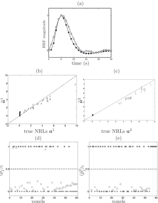
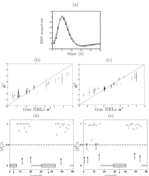
As shown in Figs. [2-5](a), all HRF estimates obtained using the four different models match the canonical time course hc pretty well. Figs. [2-5](b) show

the corresponding NRL estimates that we obtained from models M1-M4,

respectively in response to condition 1 while Figs. [2-5](c) summarize the same results for condition 2.

Since the artificial fMRI time courses were synthetised using aGaGMM prior and some correlated noise, it is not surprising that the estimation performed under model M1 provides the most accurate NRL estimates. Let us remark

that the NRL estimates have a small but not negligible amount of bias, which is due to the bias/variance trade-off arising in the Bayesian approach in the non-asymptotic case. Nonetheless, we have checked that the bias tends to zero when the SNR increases.

4.1.3 Influence of the noise model

Figs. [2-3](b)-(c) illustrate the impact of the noise model: a more accurate estimation of the NRLs, with smaller error bars and lower mean square er-ror, is observed in Fig. 2(b)-(c) compared to Fig. 3(b)-(c), that is for model

M1 compared to model M2. This is a direct consequence of accounting for

serial correlation in M1. The same conclusion holds when looking at Figs.

[4-5](b)-(c), so irrespective of the prior mixture type. As regards the HRF esti-mate (compare Figs. [2-3](a)), the noise model has only little influence on the recovered shape, as already advocated in (Marrelec et al., 2003). As regards AR parameters, the estimated first order coefficients (ρi)i are close to the true

values in every voxel for both models M1-M3 (results not shown).

We also assessed the sensitivity and the specificity of the four models. Figs. [2-5](d)-(e) show the posterior mean estimates (¯pm

j )1 of deciding that voxel Vj

lies in class 1, i.e., is activating for models M1-M4 and conditions 1 and 2,

respectively. These results confirm our expectations: the modelling of the tem-poral correlation significantly improves both the sensitivity and the specificity. A higher/lower value of (¯pm

j )1 is obtained with M1-M3 when Vj is truly

activating/non-activating (compare Figs. [2-3](d)-(e) for GaGMM priors or Figs.[ 4-5](d)-(e) for GMM priors). This means that models M1-M3 provide

lower false positive (FP) and false negative (FN) rates than models M2-M4,

respectively. This effect is stronger in condition 1. This is in agreement with the idea that the precision of the noise model plays a more important role at a lower SNR.

4.1.4 Influence of the mixture prior

Not surprisingly, the estimated NRLs are recovered more accurately using the true prior mixture (M1-M2): compare Figs. [2-4](b)-(c) one to another for an

AR(1) noise model and observe the difference in Figs. [4-5](b)-(c) for a white noise model. This effect is much more important at low SNR, i.e., for condition 1. However, we have checked that when the true NRLs of the activating voxels follow a Gaussian distribution, the estimated shape and scale parameters of the gamma density in theGaGMM mixture provide close estimates of the mean and variance parameters of the uncentered Gaussian distribution (results not shown).

We are now interested in assessing the differences between M2 and M3. The

purpose of such a comparison is to decide whether or not a good mixture type provides more accurate and sensitive results than a precise noise mod-elling. Contrasting Figs. [3-4](b) allows us to note that M2 outperforms M3 in

terms of accuracy of estimation for the first experimental condition. The NRLs attached to the non-activating voxels are over-estimated, leading to a much

(a) HR F magnitud e 0 5 10 15 20 25 0 1 time (s) (b) (c) ba 1 ba 2 true NRLs a1 _{true NRLs a}2 (d) (e) (¯p 1 j) 1 (¯p 2 j) 1 voxels voxels

Fig. 2. Estimation results on the simulated data using model M1. (a) HRF

re-sults: Symbols¥ and ◦ represent the true h_c and its corresponding HRF estimate,

respectively. (b)-(c): NRL estimates for conditions 1 and 2, respectively. True val-ues appear on the x-axis and estimated valval-ues on the y-axis. The error bars follow Eq. (10). (d)-(e): PM estimates of activation probabilities ¯pm

j (◦ symbols) for the

conditions 1 and 2, respectively. Symbols ∗ depict the true class attached to each voxel.

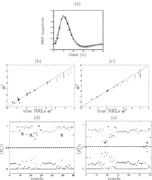
larger bias. In case of high SNR arising for the second condition, the com-parison of Figs. [3-4](b) is less clear. The small NRLs are still over-estimated but the large ones are better estimated using M2 in some cases (e.g., voxels

27, 58, 60). In terms of detection, Fig. 3(d) shows that a single false nega-tive (voxel 3) is retrieved by model M2 for condition 1, while five FNs are

found by model M2, as shown in Fig. 4(d) (voxels 3, 6, 19, 26, 32). Hence,

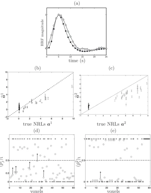
There-(a) HR F magnitud e 0 5 10 15 20 25 0 1 time (s) (b) (c) ba 1 ba 2 true NRLs a1 _{true NRLs a}2 (d) (e) (¯p 1 j)1 (¯p 2 j)1 voxels voxels

Fig. 3. Simulation results using model M2. The same legend as in Fig. 2 holds. Only

one FN voxel is present, indicated with an upward arrow.

fore, we conclude that introducing an inhomogeneous prior mixture is more powerful than modelling the serial correlation as regards both estimation and detection.

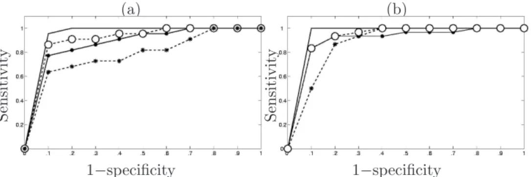
Receiver-operator-characteristic (ROC) curves have been also computed to quantitatively evaluate the differences between models M1-M4. Fig. 6

illus-trates and confirms that model M1provides the most sensitive detection when

specificity is fixed and a better specificity at a given sensitivity. These ROC curves also validate that model M4is the less sensitive and the less specific out

of the four models. Finally, model M2 outperforms M3 and provides better

results in terms of sensitivity and specificity, irrespective of the stimulus type. Fig. 6(a)-(b) allows us to claim again that the noise model has a stronger

im-(a) HR F magnitud e 0 5 10 15 20 25 0 1 time (s) (b) (c) ba 1 ba 2 true NRLs a1 true NRLs a2 (d) (e) (¯p 1 j) 1 (¯p 2 j) 1 voxels voxels

Fig. 4. Simulation results using model M₃. The same legend as in Fig. 2 holds. FN voxels are indicated by upward arrows.

pact in detection at low SNR since the distance between continuous and dotted lines is larger in Fig. 6(a) than in Fig. 6(b), except at very low specificity (0.1). This holds whatever the mixture type.

4.2 Deactivation modelling

Our purpose was to compare an inhomogeneous two-class mixture model with its three class extension. In the latter case, a third class is used to account for putative deactivation phenomenon arising for instance during sustained bursts of interictal epileptiform activity (Bagshaw et al., 2005; B´enar et al., 2006).

(a) HR F magnitud e 0 5 10 15 20 25 0 1 time (s) (b) (c) ba 1 ba 2 true NRLs a1 true NRLs a2 (d) (e) (¯p 1 j) 1 (¯p 2 j) 1 voxels voxels

Fig. 5. Simulation results using model M₄. The same legend as in Fig. 2 holds. FP and FN voxels are indicated by downward and upward arrows, respectively.

Suitable artificial fMRI datasets were simulated accordingly. We considered a ROI consisting of J = 60 voxels. Let J−1,m, J0,m J1,m be respectively the

number of deactivating, non-activating and activating voxels in response to condition m. We set (J1,1, J−1,1) = (28, 19) and (J1,2, J−1,2) = (32, 12), so that

(J0,1, J0,2) = (13, 16). We simulated the NRLs as follows:

activating voxels : a1

j ∼ G(3, 1), a2j ∼ G(5, 2)

non-activating voxels : a1,2_j ∼ N (0, 0.1)

deactivating voxels : −a1

j ∼ G(5, 4), −a2j ∼ G(5, 4)

(a) (b) Sen si ti v it y Sen si ti v it y 1−specificity 1−specificity

Fig. 6. (a)-(b): ROC curves associated to the four different models for condition 1 (a) and condition 2 (b), respectively. Continuous line, interrupted line with ◦, continuous line with • and interrupted line with ∗ represent the ROC curves for models M1-M4, respectively.

fMRI time series. The only difference concerns the noise type, which is white, Gaussian and homogeneous in space to save computation time (∀j, σ2

j = 0.3).

Hence, model M2 and M5 (see Table 1) were tested and compared in terms

of estimation, detection performance and evidence.

The HRF estimates corresponding to models M2-M5 are shown in Figs.

[7-8](a), respectively. These estimated time courses appear very close to the true HRF shape. Figs. [7-8](b)-(c) show the NRL estimates related to conditions 1 and 2, computed for model M2 and M5, respectively. First, we observe that

M2 provides under-estimated NRLs for activating voxels but over-estimated

parameters for deactivating ones, irrespective of the stimulus type. The esti-mated error bars also appear significantly larger when deriving from M2. In

contrast, model M5 provides more reliable NRL estimates with smaller error

bars, as illustrated in Fig. 8-(b)(c). Also, the mean square error is decreased for the NRLs corresponding to deactivating and non-activating voxels.

Fig. 7(d)-(e) demonstrates that model M2reports a few FN voxels (see upward

arrows). All these voxels have small NRL coefficients, inducing their assign-ment to class 0. More importantly, we observe that the truly non-activating and deactivating voxels are mixed in class 0, irrespective of the condition. Fig. 8(d)-(e) reports the posterior mean estimates (¯pm

j )i (see (8)), which are

then combined to get the final classification according to the MAP criterion (qbm

j )MAP (see (9)). As indicated on these graphs, model M5 produces an

ac-curate classification. Fig. 8(d)-(e) respectively show the presence of three FN voxels for condition 1 and only two FNs for condition 2. These classification errors could be explained by the low values taken by the true NRL coefficients in these voxels, making likely the assignment to class 0.

Finally, note that modelling the third class induces a higher computation time. In our simulations, inferring the parameters of models M2 and M5 takes

about 6 and 11 minutes, respectively. If the ROI is large or if the experimental paradigm involves numerous conditions, it seems reasonable to start with a

careful analysis of the paradigm to anticipate potential deactivations before inferring upon parameters of M5 instead of M2.

(a) HR F magnitud e 0 5 10 15 20 25 −0.2 0 0.2 0.4 0.6 0.8 1 1.2 time (s) (b) (c) ba 1 ba 2 true NRLs a1 _{true NRLs a}2 (d) (e) (¯p 1 j)1 (¯p 2 j)1 voxels voxels

Fig. 7. Simulation results using model M2. FN voxels are indicated by upward

arrows. The truly deactivating voxels that have been mixed in class 0 are surrounded by rectangle.

4.3 Bayesian model comparison

More formally, from a statistical point of view we compare models M1-M5

by computing sample-based approximations to the model evidence p(y | Mm).

That allows us to derive Bayes factors BFmn as ratios of model evidence (see

Appendix C for computational details). Bayes factor provides us with good statistical summary for model comparison. As reported in Table 3, there is a strong evidence in favour of Model M1. More interestingly, our

(a) HR F magnitud e 0 5 10 15 20 25 −0.2 0 0.2 0.4 0.6 0.8 1 1.2 time (s) (b) (c) ba 1 ba 2 true NRLs a1 _{true NRLs a}2 (d) (e) (¯p 1 j)1 (¯p 2 j)1 voxels voxels

Fig. 8. Simulation results using model M5. The same legend as in Fig.2 holds. FP

and FN voxels are surrounded by rectangles (3 FNs in (d) and 2 FPs in (e)). ◦, · and ∗ symbols represent (¯pm

j )1 , (¯pmj )−1 and (¯pmj )0, respectively.

M2 with M3 using Bayes factor (line 2, Table 3). This also holds for the

comparison between the two-class and the three-class mixtures, M2 and M5

Table 3

Values of the integrated log-likelihood log p(y | Mm) computed from a stabilized

version of the harmonic mean identity (Raftery et al., 2007) for models M_m with

m ∈N∗

5. Model comparison based on the computation of Bayes factors log BFmn=

log p(y | Mm) − log p(y | Mn) for every pair (m, n). NR stands for Not Relevant.

Model m log p(y | Mm) Fig. # log BFmn, n = 1 : 4

M1 −199 Fig. 1 NR 18 316 400 M2 −217 Fig. 2 −18 NR 298 378 M3 −515 Fig. 3 −316 −298 NR 378 M4 −595 Fig. 4 −400 −378 −80 NR M2 −700 Fig. 6 M5 −344 Fig. 7 log BF₅₂= 356

5 Results on real fMRI data

5.1 fMRI experiment 5.1.1 MRI settings

The experiment was performed on a 3-T whole-body system (Bruker, Ger-many) equipped with a quadrature birdcage radio frequency (RF) coil and a head-gradient coil insert designed for echo planar imaging (EPI). Functional images were obtained with a T2*-weighted GE-EPI sequence with an acqui-sition matrix at the 64 × 64 in-plane spatial resolution and 32 slices. A high-resolution (1 × 1 × 1.2 mm3_{) anatomical image was also acquired for each}

subject using a 3-D gradient-echo inversion-recovery sequence.

5.1.2 Experimental paradigm and contrast selection

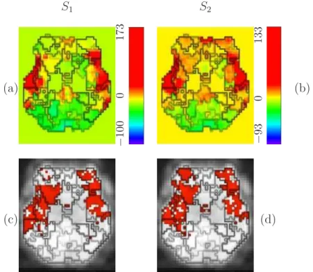
The reader may refer to (Dehaene-Lambertz et al., 2006) for details about this fMRI experiment. In short, the motivation of this study was to measure the reduction in the neural activity subserving a cognitive representation when this representation is accessed twice (the so-called “repetition suppression” effect), resulting in a detectable adaptation of the measurable signal in fMRI (Grill-Spector and Malach, 2001; Naccache and Dehaene, 2001). The experiment consisted of a single session of N = 216 scans lasting TR = 2.4 seconds each. Sixty sentences presented in a slow event-related design (SOA=14.4s) were recorded. Each sentence (S1) could be repeated two (S2), three (S3)

or four (S4) times in a row. The main goal of our subsequent analysis was

a given sentence either decrease with repetition or keep a constant magnitude across the repetitions. Second, we were interested in inferring the hierarchical temporal organisation from the parcel-based HRF estimates along the superior temporal sulcus (STS).

Since the most significant habituation effect occurs between the first and sec-ond sentence repetitions, we modelled the four csec-onditions S1-S4 but we only

studied the contrast S1− S2.

5.2 Pre-processings

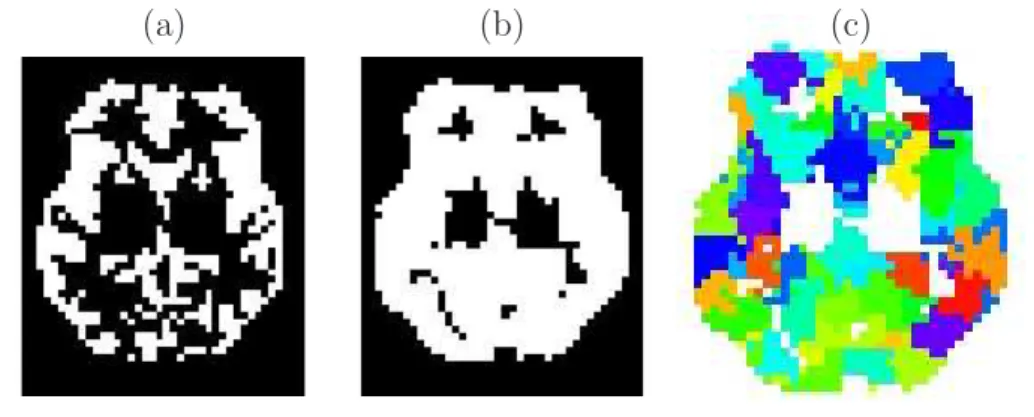
As explained in Subsection 2.1.1, the grey matter’s mask was first com-puted (see Fig. 9(a)) and then dilated using a 4mm-radius sphere to account for the width of the cortical ribbon. Fig. 9(b) shows the result of this step. The resulting mask Ma contains 19719 voxels at the fMRI resolution.

(a) (b) (c)

Fig. 9. (a): Slice of Subject 1’s anatomical mask (z = −4 mm). (b): its dilated version M_a to match the functional resolution. (c): corresponding parcellation in the same slice. Each colour codes for a different parcel.

We checked that for nine out of ten subjects the raw fMRI data were motion-free approximately. All T1-weighted MRI images were normalised onto the MNI

template and functional images were transformed accordingly. fMRI volumes were also spatially smoothed using a Gaussian kernel with F W HM = 6 mm along each direction. A first level analysis was performed for each subject using SPM2. The GLM modelled the four presentations of a given sentence with two regressors (the canonical HRF and its time derivative). Then, the parcellation was computed from the parameter estimates of this analysis. We chose a relevant F-contrast c = [1, 0, −1, 0, · · · ; 0, 1, 0, −1, · · · , ...] to study the habituation effect between the first and second presentations of a given sentence (S1− S2). Fig. 9(c) depicts an axial view of this parcellation for the

same slice (z = −4 mm).