Critical roles of constitutive laws and numerical models in the design and development of Arctic offshore installations

Publisher’s version / Version de l'éditeur:

Vous avez des questions? Nous pouvons vous aider. Pour communiquer directement avec un auteur, consultez la première page de la revue dans laquelle son article a été publié afin de trouver ses coordonnées. Si vous n’arrivez Questions? Contact the NRC Publications Archive team at

PublicationsArchive-ArchivesPublications@nrc-cnrc.gc.ca. If you wish to email the authors directly, please see the first page of the publication for their contact information.

https://publications-cnrc.canada.ca/fra/droits

L’accès à ce site Web et l’utilisation de son contenu sont assujettis aux conditions présentées dans le site LISEZ CES CONDITIONS ATTENTIVEMENT AVANT D’UTILISER CE SITE WEB.

International Conference and Exhibition on Performance of Ships and Structures

in Ice 2010 (ICETECH 2010), pp. 353-360, 2010-09-20

READ THESE TERMS AND CONDITIONS CAREFULLY BEFORE USING THIS WEBSITE. https://nrc-publications.canada.ca/eng/copyright

NRC Publications Archive Record / Notice des Archives des publications du CNRC :

https://nrc-publications.canada.ca/eng/view/object/?id=c1483535-c4ac-4445-b87e-4f50a5431f26

https://publications-cnrc.canada.ca/fra/voir/objet/?id=c1483535-c4ac-4445-b87e-4f50a5431f26

NRC Publications Archive

Archives des publications du CNRC

This publication could be one of several versions: author’s original, accepted manuscript or the publisher’s version. / La version de cette publication peut être l’une des suivantes : la version prépublication de l’auteur, la version acceptée du manuscrit ou la version de l’éditeur.

Access and use of this website and the material on it are subject to the Terms and Conditions set forth at

Critical roles of constitutive laws and numerical models in the design

and development of Arctic offshore installations

Critical Roles of Constitutive Laws and Numerical Models in the Design and Development of Arctic

Offshore Installations

Ahmed Derradji Aouat

National Research Council of Canada, Institute for Ocean Technology St. John’s, Newfoundland and Labrador, A1B 3T5, Canada

Ahmed.Derradji-Aouat@nrc-cnrc.gc.ca

ABSTRACT

Perhaps, it is time for both constitutive laws and failure criteria for ice to join efforts with numerical methods and computer power to provide a powerful simulation tool for ice engineers to calculate ice loads on Arctic structures, and subsequently investigate the response of the structure with a higher degree of confidence than ever before. Considering the power of computers today and the complexity of ice behaviour, and the subsequent response of the structure, the combined constitutive-numerical technology seems to be one of the most appropriate and effective engineering tools to calculate ice loads on Arctic offshore installations, and realistically simulate ice-structures interaction processes.

KEY WORDS:

INTRODUCTION

From a practical engineering point of view, a comprehensive design of an Arctic offshore structure (fixed or floating) should be based on two main pillars: 1) a good understanding of ice regimes, ice types, and ice behaviour through experimentation and observation of ice dynamics and mechanics in its natural conditions, and 2) a good prediction model for the response of the offshore structure when subjected to ice floes impacts. Ice-structure interactions problem is fundamentally a multi-physics issue where the interplay between ice, structure, and the hydrodynamics effects should be understood and included in any comprehensive design of offshore platforms in ice infested waters. A comprehensive predictive methodology of the interactions between ice and marine structures is guided by at least two critical factors. They are: 1) the constitutive law (rules for ice mechanics, strength, and its failure) and the numerical capability to solve a set of equations for multi-physics and complex boundary value problems. Constitutive laws deal with the ice material behavior (elastic, plastic, and time/temperature dependency) and its damage, while numerical modeling takes into account the engineering problem, such as the geometry and boundary conditions, the hydrodynamic effects (current, waves), and the solution technique used for the governing equilibrium equations. Through the numerical component, engineering results are obtained such as the reactions of the structure; global and local ice forces, stresses and strains in various members of the structure.

The following is a reflection on a general emerging trend in predictive methodologies to forecast the magnitude (and the effects) of ice loads on offshore structures in the Arctic and sub-arctic regions (i.e.; ice infested waters). Equally important, this emerging predictive tool could well form the basis to devise actual instruments, and processes, to manage ice in the Arctic on a large scale. It is a fact that effective management of ice will help to open the Arctic and access its economical resources with less risk to the environment. For Canada, in particular, the art of ice management and ice control is to be mastered if Arctic natural resources are to be explored and developed. Existing ice management programs off the coast of Newfoundland and Labrador provide valuable lessons, experience, and expertise.

DRIVERS FOR PREDICTIVE TECHNOLOGIES

To be able to develop and effectively use multi-physics prediction methodologies for ice loads on offshore structures, one fundamental condition is required. That is a good insight into, and the proper understanding of, sea ice mechanical behaviour and its movement in nature. This is one golden key needed to realistically predict ice floes interactions with offshore structures, how ice loads are generated, and how ice can be managed and controlled.

Over the year, many field and laboratory scientific research programs have shed a good light into the physics of ice, its mechanical behaviour, strength, damage, and fracture (in this paper, there is a fundamental

difference between “damage” and “fracture”, as will be explained below). Other programs, targeted studies of ice types, ice regimes and

movement of ice floes, formation of ice ridges, icebergs frequency and distribution. The field for ice engineering is information rich; some scientific investigations go back to late 1800s. The tragedy of the Titanic in early 1900s was a strong wake up call for ice engineers, it demonstrated the risks and the severe consequences associated with ice and ice loads. The latter part of the 1900s, work on ice management and ice loads was driven by marine transportation safety and safe access to hydrocarbon energy resources in the northern hemisphere. For the moment, it is realistic to assume that field and laboratory ice testing programs will continue, and it may intensify in the future since global warming is changing the natural conditions of ice rapidly (realistically, what we know about Arctic ice today may change drastically in few years due to global warming).

Chronologically, in recent times, from early field and laboratory testing (1960s to 1980s), many empirical and analytical models have been developed to calculate ice pressures. Examples include equations by korzhavin (1962), Ralston (1978), Croasdale (1980), Bercha et al. (1985), and Sanderson (1988). Ice testing and analysis of test data was the first fundamental step taken toward to develop predictive empirical and analytical equations to predict ice loads on offshore installations. Over the last two decades, and with the help of computers, a second fundamental step was taken towards to develop new methods to predict ice loads and ice effects on offshore platforms. That is the numerical solutions, such as Finite Elements Methods (FEM). The basic purpose and advantage of numerical methods (not analytical or theoretical closed form solutions) is to provide predictions for complex ice-structure interactions taking into account the natural, geometric, and boundary conditions of the ice. An additional advantage is its attempt to reduce conservatism produced by empirical and analytical equations. Equally important, numerical methods can predict ice floes movements, its interactions with various offshore installations (fixed or floaters), including hydrodynamic effects, and provide an overall solution. Ice mechanics and ice numerics are two fundamental factors that play critical roles in any modern and effective ice engineering predictive and/or design methodology. These two factors complete one another, and they need each other.

In order to develop realistic predictive models, the engineering framework is two folds 1) understanding the current state of the art for ice behaviour through field and laboratory testing, and 2) predicting its future behaviour using numerical solutions. This thinking is holistic; it is a multi-physics approach that includes ice, water, offshore structure, and the natural conditions such as current, waves, and wind. For the lack of a better terminology, this holistic constitutive-numerical method may be called “Ice Predictive Technology, IPT“. Essentially, IPT is an all-inclusive system of thinking with the objective to include ice information and known facts into one model.

For clarity, in its narrow and limited definition, constitutive model means a stress-strain curve; a relationship between applied loads and the resulting displacement (deformation). However, in its larger definition, constitutive laws are similar to a constitutional document for how ice behaves. Guided by this constitution, numerical methods use mathematics to predict ice behaviour, ice movement, and ice loads.

The constitutive model is the law and the numerical model is the tool used to enforce that law. It is similar to governance and management

models in business organizations. The constitution provides governance “how ice should behave”, and the numerical model provides mechanisms “operational policies” to enforce the constitution”.

SCOPE

In this work, through examples, the critical roles of both constitutive laws and numerical solutions are highlighted. In these examples, the main focus will be on three particular items. They are: 1) the numerical basin (numerical tank full of water), 2) the constitutive law (how ice behaves in the numerical tank), and 3) the numerical experiment (simulations of interactions of ice floes with offshore platforms). Furthermore, several other examples are given throughout the paper for more illustrations. It may be worth noting that all examples given in this document are taken from simulations of actual projects conducted at the NRC-IOT over the last three to five years.

In the literature, many constitutive laws and many numerical solutions exist. However, the work in this paper is focussed on a visco

elastic-plastic constitutive law for ice (Derradji-Aouat et al., 2000), a multi-surface failure criterion for ice (Derradji-Aouat, 2003), and a numerical tool called the Marine Dynamics Virtual Laboratory (MDVL, Derradji-Aouat, 2001). The MDVL is made up of a bundle of software that exists at the NRC-IOT, such as ANSYS (www.ansys.com) and LSDYNA (www.lsdyna.com). Other constitutive laws and numerical tools from the literature can be combined in the same way as reported in this paper.

Within the current state of the art, the main concern of any numerical predictions, however, is in its uncertainty. A future development, although starting, is assessing the accuracy of these holistic predictive numerical methods through benchmarking, validation, verification, and Experimental Uncertainty Analysis, EUA (Derradji-Aouat et al., 2004).

CONSTITUTIVE LAW, DAMAGE, AND FAILURE OF ICE

A constitutive model is the mathematical description of how ice deforms and fails under external loads. The constitutive law given in this section was developed in two phases. The 1st phase was based on two main pillars: They are: 1) Test results of cyclic and repeated creep experiments on columnar-grained ice (tests using ice samples in the cold room), and 2) the uniaxial delayed elastic formulation produced by Sinha (1978). Together, the two pillar state that, under external loads, the total deformation of ice is divided into 4 strain components:

c p d i t

ε

ε

ε

ε

ε

=

+

+

+

Where εt, εe, εd, εv and εc are the total, instantaneous elastic, visco-elastic (delayed time dependent recoverable deformation) visco-plastic (time dependent permanent deformation), and a deformation component due to damage (damage is inter and intra grain boundary

cracking), respectively. For detailed mathematical derivation of each

strain component, see Derradji-Aouat et al. (2000). Instantaneous elastic strain (εe) is due to lattice deformation, the delayed elastic strain (εd) is due to grain boundary sliding, the visco-plastic strain (εv) is due to crystalline structural changes such as movement of dislocations. The strain component induced by damage (εc) is due to inter and intra crystalline cracks. It is a permanent when small grain boundary cracks open and don’t close back when the external loads are removed. However, they are elastic when the micro-cracks heel back when external loads are removed. Damage and healing at the grain boundaries are formulated mathematically in the constitutive law on the basis of crack kinetics theory produced by Krausz and Krausz (1989). For clarity, the expressions “time-dependent”, “creep”, and “visco” are used as synonyms. The terms elastic and plastic are defined as per their traditional definition (Hill, 1950): “elastic strains” means “recoverable strain”, while “plastic strain” means “permanent strain”.

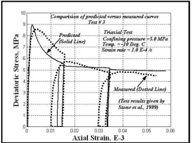
Figure 1 shows two examples for how the constitutive law predicted successfully the deformation and damage of ice samples at low strain rates (ice samples tested in the cold room). The first example (Figure 1a) shows how the peak of the stress-strain curves (the strength) was predicted for uniaxial tests on columnar-grained ice samples. More importantly, the figure shows that the strength was predicted well (accurately) without the use of any failure criterion. The damage

component (ε c) predicted the peak of the curve. The second example

(Figure 1b) shows the capability of the model to predict ductile behaviour (residual stresses). Also, it shows the ability of the model to predict the plastic strains (permanent deformation) after each unloading-reloading cycle in triaxial cold room tests on isotropic ice.

Figure 1a. Predicted versus measured stress strain curves (uniaxial tests on columnar grained ice in the cold room by Sinha, 1982)

Figure 1b. Predicted versus measured loading-unloading (plasticity) curves (triaxial tests on isotropic by Stone et. al, 1989)

Equation 1 does not work well for high strain rates “or high loading rates”. At high strain rates, > 10-3/s, the time dependent terms in Eq. 1 (εd, εv and εc,) do not have enough time to develop. Only the instantaneous elastic component, εe, can be calculated. At high strain rates, Eq. 1 predicts only elastic deformation, and it can’t predict the brittle failure of ice. Experimental data in the literature show that at

high strain rates, ice behaves primarily as a linear elastic material with a brittle model of failure (Cammaert and Muggridge, 1988).

Tests by Sinha, 1982

Constitutive law predictions

For a linear elastic behaviour of ice with brittle mode of failure, the 2nd phase of the constitutive law was developed. Basically, Eq. 1 was complemented by a multi-surface brittle failure criterion (Derradji-Aouat, 2003):

0

*

*

*

J

+

F

I

+

F

I

=

F

Where J2D, I1 and I2 are the 2nd invariant of deviatoric stress tensor, the first and second invariant of the stress tensor, respectively. F1, F2 and F3 are multiplying factors that are function of confining pressure,

strain rate, and temperature (note that the tensor notation in Eq. 2 is the

same as in Desai and Siriwardane, 1984).

Theoretically and historically, the multi-surface failure model (Eq. 2) was developed on the basis of Prevost’s (1978) nested yield elliptical anisotropic surfaces for soil plasticity. In turn, Prevost based his model on the nested circular isotropic yield surfaces theory provided Mroz (1967). In turn, Mroz (1967) based his multi-surface equations on the classical plasticity by Hill (1950). For a good literature review for the multi-surface plasticity theories for metals and its evolution to include soils, see Derradji Aouat (1988). For the evolution of the multi-surface model from soils to include ice failure, see Derradji-Aouat (2003).

q

_{ellipse j+1}

ellipse j

P-4

P-n

Figure 2. Elliptical multi-surface failure envelops for ice

It is important to point out that the classical theory of plasticity (Hill, 1950) has three rules and four conditions. The 3 rules are a yield criterion, a hardening/softening law, and a flow rule. The 4 conditions are irreversibility, consistency, normality and continuity. Without these fundamental plasticity rules and conditions, the present constitutive model and failure criterion (Eqs. 1 and 2) cannot be used.

The multi-surface material yield theory has a good lineage, historical development since 1940s, and it is transparent (equations can be traced back to their original source, re-derived, and used independently), and it has been proven to be universal and versatile. Universal in the area of solid mechanics since it was used in metals (Mroz, 1967), soils (Prevost, 1978), ice (Derradji-Aouat, 2003), and various other materials. Also, it is versatile because it formulates yielding and failure in the 3-D stress space, including any stress path. Figure 2 shows various stress paths (P1, P2, …, and Pn) in the q-P space (compression, tension, extension, shear, confined, …etc).

Initial Hydrostatic Pressure, Po

P

P-1

Po

Together, Eqs 1 and 2 have the ability to mathematically predict the mechanics and failure of ice for any strain rate, any temperature, any loading path, and they take into account ice isotropy and anisotropy (columnar-grained ice, isotropic ice), plasticity, damage, and fracture (fracture will be further explored in the numerical section below)1. This is the true strength of the present constitutive model (it is

versatile). Its versatility is shown through examples in the sections

elow.

hile the st rate and brittle mode of failure is predicted by equation 2.

UMERICAL MODEL

that were used to develop the MDVL concept erradji-Aouat, 2001).

igure 3b. Waves in the numerical tank, model at time = t

b

By using the above two equations (1 and 2), the slow rate and ductile time dependent behaviour of ice is captured by equation 1, w fa

N

To model actual ice engineering problems, the constitutive model for ice should be implemented (integrated) into a numerical code, such as FEM (either implicit or explicit). Explicit FEM allows ice elements to break away, simulate fracture, and track the movement of discrete broken ice pieces. Depending on the software programming skills used, the implementation process could be time consuming and somewhat difficult. The constitutive model described in this paper was implemented in both ANSYS (Martonen et al., 2003) and LS-DYNA (Wang and Derradji-Aouat, 2009). ANSYS and LSDYNA are two commercial FE packages

(D

Figure 3a. Numerical tank model, model at time = 0

F

Two main differences exist between ANSYS and LSDYNA model implementations: 1) ANSYS is an implicit FE structural-mechanical

ed, e computation time increases by at least one order of magnitude.

XAMPLES AND DISCUSSION

ank

1 _{Numerically, Eq. 2 is used to predict the initiation and propagation of}

large fracture in ice floes.

code. However, LSDYNA is an explicit FE code with capability to include the hydrodynamics effects. Explicit FE is particularly good for short term and highly dynamic collisions. Implicit ANSYS FE, however, is much useful when the hydrodynamic component is not critical, and there is no need to include water (fluid) in the simulations. In addition, in LSDYNA, buoyancy and hydrodynamics effects are taken into account directly. In ANSYS, however, the buoyancy may be taken into account through assumptions for equivalent body loads and initial boundary conditions. From experience, if the fluid is includ th

E

The following are three main examples given to show how an integrated constitutive-numerical prediction methodology may look like. They are 1) the numerical t , the ice in the numerical tank,

nd the numerical experiments

a .

xample # 1: Numerical Tank

the total number f elements and speed up the CPU solution time.

hat is the same size as the NRC-IOT Clear

igure 3c. Hydrostatic pressure contours in the numerical tank

re pronounced, and e use of full CFD code is “a numerical overkill”.

E

Figure 3 shows an example for a numerical basin of 50 m long, 4 m deep, and 1 m wide. This type of tank is called “a Pseudo 2-D basin” because the width of the basin is much smaller than the other two dimensions. Pseudo 2-D tanks are usually used to limit

o Air (fluid)

Water (fluid) Wave-maker (structure)

Tank: 50 m 4 m X 1m

The Pseudo 2-D model, in Figure 3, is just an example developed specifically for this paper. However, any tank dimensions are possible. A larger tank (90 m long, 3 m deep, and 12 m wide, the same size as the NRC-IOT ice tank) was, previously, developed (Derradji, 2001). Another larger numerical tow tank (200 m long, 12 m wide, and 7 m deep was also simulated, t

Water Tow Tank, CWTT.

Pressure from 101,325 Pa (1 atm) at the water free

surface to 141,325 Pa at the tank floor

Red ~ 141,325 Pa

Blue ~ 101,325 Pa (1 atm) Waves

Movement of the wave-maker

F

The water in the tank is modelled as a fluid material. The constitutive model for the fluid is made up using a two-part equation: the 1st part relates the shear resistance (drag) to viscosity of the fluid, and the 2nd part is an Equation of State (EOS). The 1st part gives results for motions, velocities, and accelerations, while the 2nd part gives pressures and volumetric deformations in the fluid. This is not a solution for Navier-Stocks equations used by most CFD commercial codes. It is a technique used to include the effects of hydrodynamics (forces, added masses, motions, pressures, and viscosity) into account. In ice-structure interaction solutions, the proper inclusion of hydrodynamic effects is adequate because uncertainties in ice are much mo

The tank has a numerical wave maker. This is needed in the case where ocean waves and/or currents affect the movement and the trajectory of ice floes and discrete ice masses. If the wave action is not important, in particular simulation, then the wave maker routines are not activated.

ular and regular waves (http://www.nrc-cnrc.gc.ca/eng/ibp/iot.html).

r can specify displacement (or elocity) time histories for the plate.

a

To show how to build a numerical wave maker, a flat plate was used to push the water in the numerical tank (Figure 3). For example, at the NRC-IOT, the physical wave-maker in the CWTT is made up of two steel flaps and operates in 4 modes to generate various reg

ir

For the sake of discussion in this paper, the simplified wave maker (Figure 3) is made up of only one vertical plate that moves back and forth in a linear manner. The use

v

The water mass and the steel structure of the wave maker communicate information back and forth using Fluid-Structure Interactions (FSI) equations. This communication process is sometimes called “coupling” where pressure, displacements, and velocities are communicated from the water (fluid) to the wave maker (structure) and vice versa. Also, FSI equations track the instantaneous geometry of the interface between the water and the structure (for example, in the case of travelling ships, the

SI interface geometry is moving).

tions). In

tank

ny igure 4a).

he ridge stops “bobbing” and floats calmly on the surface of e water.

An ice ridge dumped nder its own gravity) in the numerical tank

ubsequently the structure either resists or collapses under ice actions.

l behaviour and boundary conditions for the tructural components.

F

To continue with the present example, the simplified numerical wave maker was pushed back and forth, in a linear manner as shown in Figure 3b. The hydrostatic pressure was calculated accurately (Figure 3c) and the solution is very stable (water pressure values were correct, and there was no coupling breaks, leaks, throughout the simula

addition, the wave heights and lengths predicted as expected.

Figure 4a. A level ice sheet and an indentor in the numerical

xample # 2: Ice in the Numerical Tank

ructure (indentor) shape/size can be placed in the tank (F E

A numerical ice sheet was placed on the water in the numerical tank (Figure 4a). Notice that a 3-D tank is used in this example, rather than the Pseudo 2-D basin used in the previous example (Figure 3). The ice sheet can be any shape and any size. One main advantage in this methodology is that by coupling water and ice (FSI), the buoyancy works automatically and accurately (through equilibrium of body loads). The ice sheet is floating on the water; no boundary conditions for ice are required. In addition to the ice sheet, FE models for a st

Another example to show how buoyancy works is given in Figure 4b, where a multiyear ice ridge (2.8 m long, 2.0 m wide by 0.6 m deep)

was dropped (under its own weight) into the water in the numerical tank. The buoyancy forces are resolved when the final equilibrium of body loads is achieved. In the simulations, the ice ridge floats and moves up and down (bobs), but that movement is decaying over time. When all kinetic energy is dissipated and body load equilibrium is achieved, t

th

Figure 4b. Buoyancy numerical experiment: (u

After ensuring that the initial hydrostatics, buoyancy and body loads are properly modelled, the next step is to numerically simulate the interactions of ice with structures. For example, if the ice sheet, in Figure 4a, moves forwards and collides with a fixed offshore platform (indentor), then ice impact loads are felt throughout the structure, and s

Numerically, the ice sheet can be moved at an initial velocity, a constant velocity, or any other prescribed velocity or displacement with time. When the ice hits the structure, stresses are calculated in both ice and the structure elements. The structure can be either rigid or flexible. Rigid means that the structure does not deform at all, and only ice deforms and breaks away after its failure. Flexibility is achieved by the use appropriate materia

s

When ice contacts the structure, a contact algorithm is needed to transfer loads and displacement from the moving ice sheet to the target structure (and vice versa). From definitions point of view, it may be worth pointing out that the term “coupling” is used when the structural elements contact the fluid elements, while the term “contact” is used when two structural elements contact each other (such as ice elements

ontact concrete or steel elements).

collide (contact) with each ther and the parent ice sheet (self contact).

c

In this paper, ice elements deform and break away from the parent ice floe after failure. The broken ice pieces may

o Water

Ice Sheet

Structure (indentor)

Water Surface

Ice Ridge

_{At time 0.0}

After hydrostatic

Ice

Water Surface Ridge

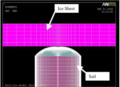
Figures 5a to 5d illustrate how contact and fracture are modelled numerically. The simulation was done using the geometry of a submarine sail penetrating through a large and thick multiyear ice sheet (the submarine sail is breaking the ice sheet upwards, Figure 5a, Derradji-Aouat and Jones, 2008). The sail of the submarine is about 11 m long and it is about 2 m wide, and as the submarine rises, the contact loads build up in both the sail and the ice sheet. The ice sheet bends upwards, and with time, ice elements fail and break away. Ice elements break as per Eq. 2, and they keep breaking as long as the stress criterion (Eq. 2) is fulfilled. The sequence of ice element breaking gives a measure for the propagation of the fracture tip (speed of the crack). As shown in Figures 5b and 5c, a large macro-crack propagated longitudinally and then another large fracture initiated and propagated in the lateral direction (corresponding animated videos from the

igure 5a. FE model for the submarine sail and the ice sheet simulations are shown in the presentation).

F

It is extremely important to distinguish between “ice damage” and “ice sheet fracture”. Damage is a softening deterioration mechanism controlled by the last term in Eq. 1, εc, while fracture is failure of an entire element controlled by Eq. 2. The terms “macro cracks” and “fracture” are used interchangeably. Also, the terms “damage” and

icro-cracks are use interchangeably as well

eet cracks) m

Figure 5b. Submarine sail penetrating through an Arctic ice sh (longitudinal fracture – initiation and propagation of

macro-Figure 5c. Submarine sail penetrating through the ice sheet

Lateral fracture

Longitudinal fracture

Ice Sheet

Sail

(Longitudinal and lateral fracture)

Longitudinal fracture

Figure 5d. Fracture (macro-cracks) in submarine sail penetrating through Arctic ice simulations study (Derradji-Aouat and Jones, 2008) Micro cracking is a damage mechanism at the ice crystals/grains level (either at grain boundaries and/or trans-crystalline micro-cracks). It is a softening mechanism, this is very apparent in post-yield stress-strain curve of ice undergoing ductile mode of behaviour (see Figure 1b).

Macro cracking, however, is the failure of an entire ice element (not just one crystal/grain). Depending on the resolution of the FE model, the element size varies from few millimetres to several meters. Equation 2 is a failure equation that results in splitting ice floes and breaking away of chunks of ice. Fracture, in this model, is instantaneous (time independent) and it is a sudden (guillotine - brittle) failure of elements. The simulations in Figure 5d are two examples for how ice fracture is simulated in the case of the submarine sail pushing upwards an Arctic ice sheet (note that the simulation results are very realistic, and at the moment, the actual results are confidential).

Example # 3: Numerical Experiments

The example given in this section is taken from a feasibility study done for a project. A large hydroelectric structure (120 m long, 40 m wide, and 40 m high) is to be built in the strait of bell isle (Derradji-Aouat, 2005). Therefore, the conditions of ice used in the simulations are the same as those corresponding to bell isle strait (Western Newfoundland and North-Eastern Quebec, Canada).

The CAD model, in Figure 6a, shows a large ice sheet pushing the structure (Derradji-Aouat, 2005). The FE model was developed using ANSYS and the simulations was performed using LS-DYNA where both constitutive law and failure criterion for ice were implemented. Figure 6b shows the simulations at its final stages when large fractures propagated through the ice sheet. Global ice loads on the vertical walls of the structure (total reactions of the structure) are given in Figure 6c.

Figure 6a. Ice sheet pushing against a vertical structure (CAD model) For local ice loads, the most interesting observation is shown in Figure 7a. Contact zones changing in time and in location (on the face of the structure) are shown; some zones are very loaded (red) while others are not (blue). In the figure, stress contours for four local contact zones (4different elements, at a given time t) are pointed out. Their corresponding local stresses are given in Figure 7b.

Both global ice load (Figure 6c) and local ice loads (Figure 7b) have a common trend. The stress curves indicate a load build up, and when ice elements fracture and break away, the load curve drops down. This is a typical trend of load curves for ice. Maximum magnitude of ice pressure is ~ 1.0 MPa, which is very realistic.

Fractures

Figure 6b. Typical simulations of fracture in the ice sheet pushing the vertical structure

Figure 6c. Global ice loads at the ice structure interface

Ice Fence

Ice Sheet

CONCLUDING REMARKS

The examples given in this paper are not by any means exhaustive, but they are versatile and they show the critical roles played by both constitutive laws and numerical models in solving complex boundary problems involving ice floes, offshore installations, and hydrodynamic effects (sea water). Using a holistic (metaphysics), transparent and reproducible approach, realistic natural interactions of ice with offshore installations can be simulated and analyzed.

Vertical Structure

120 m X 40 m X 40 m

The schools of thought on the other side of the spectrum (such as the school of thought that embraces only empirical approaches with simplifying assumptions) may argue against the complexity and costs involved in using a multi-physics solution. But, the conservatism and risks involved with extrapolation of empirical equations gave a birth and “reason d’être” for constitutive laws and numerical solutions. Naturally, for holistic constitutive-numerical solutions, a serious validation and verification efforts are needed to further reduce uncertainties and augment confidence in the simulations. This can be achieved by comparing obtained numerical predictions with experimental field and laboratory measurements. In turn, it is critical to note that, experimental data should be worthy of validation by going through Experimental Uncertainty Analysis (EUA, ISO-GUM 1995).

REFERENCES

Once the set up for the constitutive-numerical problem is completed and adequate solution is obtained, subsequent sensitivity “parametric” analysis becomes very easy and straight forwards (it is a matter of changing input files). Very fast and very cost effective parametric simulations can be performed. Third parties can use existing macros “routines” and run simulations for their specific scenarios and maintain confidentiality of their design.

Bercha, F.G., Brown, T.G., and Cheung, M.S. (1985). “Local Pressure in Ice–Structure Interactions”. In Civil Engineering in the Arctic

Offshore, San Francisco, pp. 1243–1251.

Cammaert A.B., and Muggridge D.B. (1988). Ice Interactions with Offshore Structures. Van Nostrand Reinhold, New York.

Croasdale K.R. (1980). “Ice forces on fixed offshore structures”. US

Army Corps of Engineers Laboratory, CREEL, Report No. 24-80

As ice engineers, we may be at the verge of trusting and using more the combined constitutive-numerical tool in the analysis and design of

offshore structures destined for ice-infested water. Derradji-Aouat, A., Jones, S. (2008). “Victoria Class Submarine Sail _{Ice Penetration Study”. NRC-IOT report # TR-2009-02.} Derradji-Aouat, A. (2005). “Explicit FEA and Constitutive Modelling of Damage and Fracture in Ice”. 18th International Conference on

Port and Ocean Engineering Under Arctic Conditions, (POAC 2005),

Potsdam, New York, USA.

ACKNOWLEDGMENTS

In addition to the staff of NRC-IOT facilities group, the support of several external organizations is very much appreciated. The examples in the paper are from actual R&D projects. DRDC (Defence R&D Canada) support for the submarine under the ice project is much appreciated. The contribution of Trans Ocean Gas (TOG) is recognized through the project for a hydroelectric station in the strait of bell isle, Canada. CCORE and its participants in the PIRAM project helped very much to advance our ridge numerical modeling capabilities and skills.

Derradji-Aouat, A., Izumiyama, K., Yamaguchi, H., Wilkman, G. (2004). “Experimental Uncertainty Analysis for Ice Tank Ship Resistance Experiments”. Oceanic Engineering International, 8 (2): 49-68.

Derradji-Aouat, A. (2003). “Multi-Surface Failure Criterion for Saline Ice in the Brittle Regime”. Cold Regions Science and Technology, 36 (1-3), 47-70.

Derradji-Aouat, A. (2001). “On the Development of the MDVL”. 5th

Symposium on Emerging Technologies for Fluids, Structures, and Fluid/Structure Interactions, Atlanta, Ga., USA. 349-357

Element 51836

Element 51655

Element 52107

Element 51946

Modeling of Monotonic and Cycle Behaviour of Fresh Water ice”.

Cold Regions Science and Technology, 31 (1) 59-81.

Derradji-Aouat, A. (1988). “Evaluation of Prevost’s Elasto-Plastic Models for Soils”. M.A.Sc. thesis, University of Ottawa, Canada. Dessai C.S. and Siriwardane H.J. (1984). Constitutive Laws for

Engineering Materials. Prentice-Hall Inc.

Hill R. (1950). Mathematical Theory of Plasticity. Clarendon Press. ISO-GUM (1995), “Guide to the Expression of Uncertainty in

Measurement”, International Organization for Standardization, Genève, Switzerland

Korzhavin, K.N. (1962). “Action of Ice on Engineering Structures”.

Translated by Cold Regions Research and Engineering Laboratory, CREEL, Hanover, N.H., Translation 260, 1971.

Krausz, A.S. and Krausz, K. (1989). Fracture Kinetics of Crack Growth. Kluwer Academic Publishers, Dordrecht, The Netherlands Figure7a. von Mises stress contours on the structure interface

Martonen P., Derradji-Aouat A., Maatuanen M., and Surkov G. (2003) Nonlinear FE Simulations of Level Ice Forces on Offshore Structures”. 17h International Conference on Port and Ocean

Engineering Under Arctic Conditions, Trondheim, Norway.

Mroz Z. (1967). “On the description of anisotropic work-hardening”. Journal for the Mechanics & Physics of solids, Vol. 15, pp. 163-175. Prevost (1978): “Plasticity theory of soil stress-strain relations”. ASCE

Journal for Geotechnical Engineering, Vol. 104, pp. 347 – 361. Ralston T.D (1978). “An analysis of Ice Sheet Indentation”. IAHR

proceeding. Lulea, Sweden, Vol. 1, pp. 13-31.

Sanderson, T.J.O. (1988). Ice Mechanics: Risks to Offshore Structures. Graham & Trotman Ltd., London, U.K.

Sinha, N.K. (1978). “Rheology of Columnar Grained Ice”.

Experimental Mechanics, 18(12): 464–470.

Sinha N.K. (1982). Constant strain and stress rate of columnar grained ice. Experimental Mechanics. Vol. 17, pp. 785. 802.

Stone B.M., Jones S.J., and McKenna R.F. (1989). “Damage for Isotropic Ice Under Moderate Confining Pressures”. 10th

International Conference on Port and Ocean Engineering Under Arctic Conditions, Lulea, Sweden, Vol. 1, pp. 408-418.

Figure7b. Local element stresses for the 4 zones indicated in Figure 7a. Wang J. Derradji-Aouat A (2009), “Implementation, Verification and Validation of the Multi-Surface Failure Envelope for Ice in Explicit FEA,” POAC 2009, Lulea, Sweden. Copyright ©2010 ICETECH 10. All rights reserved.