Data management of geostationary communication satellite telemetry and correlation to space weather observations

(1)

Data Management of Geostationary Communication Satellite Telemetry

and Correlation to Space Weather Observations

by

Whitney Quinne Lohmeyer B.S. Aerospace Engineering North Carolina State University, 2011

Submitted to the Department of Aeronautics and Astronautics in partial fulfillment of the requirements for the degree

of

Master of Science in Aeronautics and Astronautics at the

MASSACHUSETTS INSTITUTE OF TECHNOLOGY February 2013

Signature of Author ………... Department of Aeronautics and Astronautics January 31, 2013

Certified by ………... Kerri Cahoy Assistant Professor of Aeronautics and Astronautics Thesis Supervisor

Accepted by ……….. Eytan H. Modiano Professor of Aeronautics and Astronautics Chair, Graduate Program Committee

(2)

Data Management of Geostationary Communication Satellite Telemetry

and Correlation to Space Weather Observations

by

Whitney Quinne Lohmeyer

Submitted to the Department of Aeronautics and Astronautics on January 31, 2013 in partial fulfillment of the requirements for the degree of Master of Science in Aeronautics and

Astronautics

ABSTRACT

To understand and mitigate the effects of space weather on the performance of geostationary communications satellites, we analyze sixteen years of archived telemetry data from Inmarsat, the UK-based telecommunications company, and compare on-orbit anomalies with space weather observations. Data from multiple space weather sources, such as the Geostationary Operational Environmental Satellites (GOES), are compared with Inmarsat anomalies from 1996 to 2012. The Inmarsat anomalies include 26 solid-state power amplifier (SSPA) anomalies and 226 single event upsets (SEUs). We first compare SSPA anomalies to the solar and geomagnetic cycle. We find most SSPA anomalies occur as solar activity declines, and when geomagnetic activity is low. We compare GOES 2 MeV electron flux and SSPA current for two weeks surrounding each anomaly. Seventeen of the 26 SSPA anomalies occur within two weeks after a severe space weather event. Fifteen of these 17 occur after relativistic electron events. For these fifteen, peak electron flux occurs a mean of 8 days and standard deviation of 4.7 days before the anomaly. Next, we examine SEUs, which are unexpected changes in a satellite’s electronics, such as memory changes or trips in power supplies. Previous research has suggested that solar energetic protons (SEPs) cause SEUs. However, we find that SEUs for one generation of satellites are uniformly distributed across the solar cycle. SEUs for a second generation of satellites, for which we currently have only half a solar cycle of data, occur over an order of magnitude more often than the first, even during solar minimum. This suggests that SEPs are not the primary cause of SEUs, and that occurrence rates differ substantially for different satellite hardware platforms with similar functionality in the same environment. These results will guide design improvements and provide insight on operation of geostationary communications satellites during space weather events.

Thesis Supervisor: Kerri Cahoy

(3)

ACKNOWLEDGEMENTS

I would like to acknowledge my parents, Melody and Bill Lohmeyer, for always supporting me and playing a critical role in my success. Dr. Fred DeJarnette, my undergraduate advisor, who’s mentoring made long-term goals become reality, and to whom I dedicate this thesis. I would also like to thank my advisor, Kerri Cahoy, for her continuous mentoring throughout my time at MIT, and during the summer before my first semester. Additionally, I would like to thank Leonard Bouygues, Carolann Belk, Gina Annab, Natalya Brikner, Ingrid Beerer, and Qiaoyin Yang for their love and friendship, which I will indefinitely cherish.

Furthermore, I would like to acknowledge Dan Baker, Yuri Shprits, Mark Dickinson, Marcus Vilaca, Janet Greene, Cathryn Mitchell, Joe Kinrade, the Invert Centre for Imaging Science at the University of Bath, Greg Ginet, Anthea Coster, Trey Cade, the Inmarsat Spacecraft Analysts, and Joseph Ditommaso for their support. I would also like to thank NOAA, LANL, ACE, SIDC and the World Data Center for Geomagnetism for access to their space environment databases. Lastly, I would like to thank NSF, MIT, and Inmarsat for funding this work.

(4)

LIST OF ACRONYMS

ACE – Advanced Composition Explorer ACS – Attitude Control System

AMER – Americas Region AOR – Atlantic Ocean Region APAC – Asian Pacific Region CME – Coronal Mass Ejection DST – Disturbance Storm Time Index EMEA – Europe Middle East Africa Region EPAM – Energetic Ion and Electron Instrument

EPEAD – Energetic Proton, Electron and Alpha Detector EPS – Energetic Particle Sensor

ESA – European Space Agency ESD – Electrostatic Discharge

ESP – Energy Spectrometer for Particles EUV – Extreme Ultraviolet Sensor GCR – Galactic Cosmic Rays GEO – Geostationary

GOES – Geostationary Operational Environmental Satellites HEPAD – High Energy Proton and Alpha Particle Detector IMF – Interplanetary Magnetic Field

IOR – Indian Ocean Region

LANL – Los Alamos National Labs

MAG – Magnetic Field Vectors Instrument and Data MAGED – Magnetospheric Electron Detector

MAGPD – Magnetospheric Proton Detector PAC – Pacific Region

POR – Pacific Ocean Region

RTSW – Real Time Solar Wind System SEM – Space Environment Monitor SEP – Solar Energetic Protons SEU – Single Event Upsets

SIDC – Solar Influences Data Center SIR – Stream Interaction Regions

SIS – High Energy Particle Fluxes Instrument SPE – Solar Proton Events

SPENVIS – Space Environment Information System SSB – Space Studies Board

SSPA – Solid State Power Amplifier STK – Satellite Tool Kit

SWEPAM – Solar Wind Electron, Proton, and Alpha Monitor SWPC – Space Weather Prediction Center

TDRS – Tracking Relay Satellite System XRS – X-Ray Sensor

(6)

LIST OF FIGURES

Figure 1: Inmarsat Satellite Locations and Coverage

Figure 2(a,b): The GEO orbit of two of Inmarsat’s satellites, one satellite is designated in pink and the other satellite in yellow

Figure 3: The Solar Cycle

Figure 4: Example of Dst phases of activity in early November 2004 [NASA SPOF, 2006] Figure 5: Annual sunspot number and Ap days >=40 [Allen, 2004]. Sunspot number is shown on the left vertical axis, and Ap is shown on the right vertical axis.

Figure 6: The Geomagnetic Cycle

Figure 7: Saturation curve of an amplifier [Elbert, 2002]

Figure 8: EADS Astrium L-Band SSPA with dimensions of 217 mm x 107 mm x 47 mm Figure 9: Satellite Age at time of SSPA Anomaly including anomalies that occur within two years of launch [Lohmeyer, 2012].

Figure 10: Single Amplitude Spectrum of Nominal SSPA Figure 11: Single Amplitude Spectrum of Anomalous SSPA Figure 12: Eclipse Seasons [CNES, 1979]

Figure 13: Satellite Local Time for the twenty-six SSPA anomalies. The radial distance from the center of the plot shows the number of anomalies that occurred, as at local midnight.

Figure 14: SPENVIS AE-8 Radiation Model with several Inmarsat locations noted.

Figure 15: SSPA Anomalies and Severe Space Weather Events. Severe Space Weather events are defined in Table 7 and listed in Appendix A-D.

Figure 16: Sunspot number for Solar Cycle 23 and Solar Cycle 24. Raw Sunspot Number (blue), Smoothed Sunspot Number (red), Inmarsat SSPA Anomalies (green points), and the Inmarsat SSPA Anomalies that occur within the first two years after launch (black points).

Figure 17 (a,b): Yearly SSPA anomaly totals per satellite fleet (yellow and green bars), plotted with smoothed sunspot number (blue line). Figure 16(a) includes anomalies that occur within two years of launch and Figure 16(b) excludes anomalies that occur within two years of launch. Figure 18: SSPA anomalies per year per satellite in Fleet A, from 1996 to 2012. The number of anomalies per year is divided by the number of satellites in operation, respectively. The satellite fleet has experienced an entire solar cycle, whereas the fleet B has not.

Figure 19: SSPA Anomalies per year per satellite and the LANL ESP log of 2 MeV Electron Flux. The LANL ESP measurements are from 1996-2009.

Figure 20: Fleet A SSPA anomalies per year per satellite and the geomagnetic cycle. Fleet B SSPA anomalies are not shown, as they first occurred in 2006, after which the geomagnetic cycle has remained quiet. The number of anomalies per year is divided by the number of satellites in operation, respectively. This normalization explains why the range of the ordinate is 0 to 0.8.

(7)

Figure 21(a-c): The Kp, Dst, and solar wind speed at the time of all 26 SSPA anomalies. Blue anomalies occurred during first two years of satellite operation and are considered to be due to the launch environment.

Figure 22: The 2 MeV electron flux rates two weeks before and after each of the SSPA anomalies. The 2 MeV electron flux rate at the time of each SSPA anomaly is shown by the black squares.

Figure 23: 2 MeV Electron Flux during SSPA Anomaly for five days prior to and one day after an anomaly plotted on the left vertical axis, and SSPA current plotted on the right axis. The GOES 2 MeV electron flux is the blue line, the SSPA current is the dotted green line, and the anomaly is marked with a red line.

Figure 24(a,b): 2 MeV Electron Flux during SSPA Anomaly for two weeks before and after an anomaly plotted on the left vertical axis, and SSPA current plotted on the right axis. Figure 23(a) and 23(b) represent two different anomalies on two distinct satellites. The GOES 2 MeV electron flux is the blue line, the SSPA current is the dotted green line, and the anomaly is marked with a red line.

Figure 25: 30 MeV Proton Flux during SSPA Anomaly

Figure 26: The distribution of 10 MeV SPEs from 10 – 10,000 pfu throughout the solar cycle and can be found in Appendix B and Appendix E-G

Figure 27: The number of SPEs per month measured from GOES, between 1996 and 2012. Dates of SPE events are in Appendix B and Appendix E-G

Figure 28: The number of SPEs per day of Bartels cycle measured from GOES, dates attached in Appendix B and Appendix E-G

Figure 29: The number of SEUs per month measured from GOES

Figure 30: The number of SEUs per day of Bartels cycle measured from GOES

Figure 31: The solar cycle and the annual number of SEUs per satellite for satellite fleet A. The different colors represent the five different satellites in fleet A.

Figure 32: Fleet A SEUs plotted with 10 MeV SPEs ranging between 10 – 10,000 pfu from 1996—2012. The red circles are 10,000 pfu SPEs, the orange squares are 1,000 pfu SPES, the green squares are 100 pfu SPEs, the blue diamonds are 10 pfu SPEs and the black asterisks are SEUs.

Figure 33: The solar cycle and the annual number of SEUs per satellite for satellite fleet B. The six different colors represent the local and remote computers on each of the three satellites in fleet B. An inverse correlation exists between the solar cycle and SEUs.

Figure 34: Fleet B SEUs plotted with 10 MeV protons ranging from 10 – 10,000 pfu from 1996—2012. The red circles are 10,000 pfu SPEs, the orange squares are 1,000 pfu SPES, the green squares are 100 pfu SPEs, the blue diamonds are 10 pfu SPEs and the black asterisks are SEUs.

Figure 35: The age (years) of the five satellites in fleet A and the three satellites in fleet B at the time of the SEU. For satellite B the SEUs on the local and remote computers are plotted

(8)

LIST OF TABLES

Table 1: Inmarsat Fleet

Table 2: Telemetry Descriptions

Table 3: Summary of Eclipse Durations

Table 4: The number of SSPA anomalies that occur during different seasons Table 5: Eclipse and SEU

Table 6: GOES Satellite Initial and Final Coverage Times

Table 7: Definition of Severe Space Weather Events used in this work.

Table 8: Number of SSPA Anomalies that occur before the given period of time between the four types of severe space weather events

Table 9: Number of SSPA Anomalies that occur after the given period of time between the four types of severe space weather events

Table 10: Geomagnetic and Solar Wind Parameters at the time of the SSPA Anomalies Table 11: Fleet A SEUs that occur 1 day, 1 week, 2 weeks, and 1 month before solar proton events of 10 MeV ranging between 10 – 10,000 pfu

Table 12: Fleet A SEUs that occur 1 day, 1 week, 2 weeks, and 1 month after solar proton events of 10 MeV protons ranging between 10 – 10,000 pfu

Table 13: Fleet B SEUs that occur 1 day, 1 week, 2 weeks, and 1 month before solar proton events of 10 MeV protons of 10 – 10,000 pfu

Table 14: Fleet B SEUs that occur 1 day, 1 week, 2 weeks, and 1 month after solar proton events of 10 MeV protons ranging from 10 – 10,000 pfu

(9)

(10)

CHAPTER 1: INTRODUCTION AND MOTIVATION

In 2008, the National Research Council published the “Severe Space Weather Events – Understanding Societal and Economic Impacts Workshop Report”. This report documents the findings from the 2007 public workshop that the Space Studies Board (SSB) of the National Academies was charged to convene to assess the nation’s ability to manage the effect of space weather and their societal and economic impacts [NRC, 2008].

One of the primary technologies of focus was the telecommunications industry. At the time of the workshop more than 250 geostationary communications satellites were in orbit, which amounted to more than a $75 billion dollar investment that delivers an annual revenue of $25 billion. Yet economics aside, this critical infrastructure is important because of the services it provides. To name a few, these satellites provide backup communication in the event of a disaster that damages ground based communications systems, they provide news, education, and entertainment to remote areas, and connect end users including military, maritime officials, or civilian subscribers.

However, the telecommunications industry is being challenged by space weather, which is not only affecting the satellites, but the satellite engineers, satellite operators and the satellite customers. For example, in 1994 Canadian Telesat experienced a space weather induced satellite anomaly when their Anik E2 satellite went off air due to an energetic electron induced discharge to the control unit. As a result, more than 100,000 dish owners and 1,600 remote communities were affected. Fortunately, the 290 million dollar satellite was restored after an intensive six month, $70 million recovery effort. Numerous other examples of space weather induced anomalies exist, yet the primary challenge lies in understanding how to quantify the effects of space weather on satellite components.

In fact, one of the workshop conclusions was that access to space weather data and as well as satellite telemetry, is the first step in better understanding the cause of satellite anomalies as they pertain to space weather. It is widely known that space weather impacts the performance of satellite systems. The ability to quantify these effects requires the analysis of both space weather and satellite anomaly data; however, the main challenge is not access to space weather data, but rather satellite anomaly data

Decades of spacecraft anomaly data sit unused in the electronic telemetry archives of major geostationary communications satellite manufacturers and operators. Telemetry comes from the Greek words tele (remote) and metron (measure), meaning to measure from a distance. These telemetry data are faithfully acquired and monitored by ground operators, and anomaly alarms are sounded should the component health data stray outside of pre-defined nominal or safe operational thresholds. The spacecraft health data are largely used in real time to help mitigate the effect of anomalies on the overall system performance and minimize impact to customers. Once the “fire” has been put out, the telemetry data are used for fault investigations, ground-based anomaly re-creation and modeling, and summaries of lessons learned.

The extensive databases of on-orbit anomalies from commercial spacecraft operators have not yet been released for scientific investigations. This is partly because scientific analyses of these anomaly data, beyond the engineering analyses for prompt detection and mitigation strategies,

(11)

are not in the immediate interest of these businesses. However, these companies are interested in using accurate real-time space weather predictions and observations for fleet operations, and thus have some motivation to contribute via research collaborations to the space weather community. Recently, Choi et al. (2012) analyzed the effects of space weather on ninety-five satellite anomalies from seventy-nine unique satellites. The study incorporated publicly available geostationary satellite anomaly data with the causes ranging from electrostatic discharge, to loss of amplifiers, complete power system failure, etc. Yet, several of these anomalies, such as those caused from failure to deploy a solar array or a safe-hold triggered by faulty ground-control software, were not likely due to space weather and should have been filtered from the analysis [Mazur, 2012]. Furthermore, although their correlation between space weather and these anomalies noted relationships between anomalies and local time, seasonal dependencies, and geomagnetic index Kp, did not normalize for the different conditions that exist between different satellite buses. Our research methodology stresses the need for normalization in the analysis of different satellite manufacturers and hardware components to assure an accurate correlation study.

For this research, we partner with Inmarsat, a telecommunications company based in the UK, to analyze satellite component anomaly data from eight satellites on two of Inmarsat’s satellite fleets. Inmarsat has been operating its fleet of geostationary (GEO) satellites for more than twenty years, and has maintained a complete archive of component telemetry and housekeeping data for more than twenty years with the primary purpose of monitoring spacecraft health and performance. Since 1996, the satellites have experienced twenty-six solid-state power amplifier (SSPA) anomalies. SSPAs are a key component in satellite communication systems, as they are used to amplify the uplink signals received by the satellite from the ground before re-transmitting the downlink signals to the users on the ground.

SSPAs have advantages in reliability, ruggedness, size and cost, compared to alternatives such as traveling wave tube amplifiers [Sechi, 2009]. There are generally two types of SSPA anomalies, “hard” failures and “soft” failures. Soft failures are generally recoverable (e.g. from power cycling) and hard failures are not. Both failures are identified when health measurements, such as SSPA current in this work, fall below a pre-defined threshold. The threshold setting is specific to particular hardware, for example, the thresholds for Fleet A SSPAs and Fleet B SSPAs are different as the satellites had different manufacturers. These health measurements are continuously recorded (e.g., hourly) and saved and then downlinked to the ground where they are monitored and archived.

It should be noted that anomalies with on-board components, such as SSPAs, are expected and are managed by all satellite operators. Anomaly rates are factored into the design of geostationary satellites and are typically mitigated through the use of on-board unit redundancy and configuration options. The current SSPA anomaly rate presented is significantly lower than that modeled as part of the design reliability analysis; hence both satellite performance and lifetime have not been impacted adversely.

In order to more accurately quantify the effect of space weather on geostationary communications satellites we focus on one type of component anomaly, solid-state power

(12)

amplifiers, as well as single event upsets (SEU). Analyzing data from 5 satellites of the same fleet, and then comparing the results with a second 3-satellite fleet allows high level insight into the effect of satellite hardware differences that are not possible in a larger, more general study. What causes these anomalies and failures? Alone, the data contain valuable information about how space weather impacts flight electronics and materials as a function of age, time, and location. The data are even more valuable when combined with space weather observations from spacecraft and from the ground. We compare the satellite anomalies with observations of the space weather environment using space weather databases from: the Geostationary Operational Environmental Satellite (GOES) database, the Advanced Composition Explorer (ACE) database, the World Data Center for Geomagnetism in Kyoto, Japan, the Solar Influence Data Center (SIDC) in Brussels, Belgium, and severe space weather events from the NOAA Space Weather Prediction Center (SWPC).

One open question is whether there are periods during the lifetime of a satellite when they may be more susceptible to anomalies, separate from the influence of space weather. For example, seven of the twenty-six SSPA anomalies occurred within the first two years of the satellites’ lifetime. Did these seven anomalies result from the taxing launch environment and orbital repositioning maneuvers that a satellite experiences within the first two years of operation, or from space weather? As we discuss in more detail in this work, anomalies that occur within the first two years of operation should first be investigated for correlation to space weather events before being categorized as “burn-in” or launch environment-related anomalies.

Inmarsat Satellite Fleet

Table 1 summarizes the three primary Inmarsat fleets, their launch date, coverage area, and longitudinal location. The fleet number I2, I3, or I4, designates Inmarsat Fleet 2, 3 and 4, along with the flight number F1, F2, F3, etc. I2 originally consisted of four satellites, however two have been decommissioned, which are the only Inmarsat satellites to have been decommissioned thus far. I3 consists of five satellites, and I4 consists of three satellites.

Both of the I2 satellites are currently positioned over the Pacific region (PAC). For the I3 satellite fleet, the coverage areas are divided into ocean regions: Atlantic Ocean Region (AOR), Indian Ocean Region (IOR), and the Pacific Ocean Region (POR). Lastly, the I4 coverage areas are divided into three regions: Asia-Pacific (APAC), Europe-Middle East-Africa (EMEA), and the Americas (AMER).

Table 1: Inmarsat Fleet

Satellite Launch Date Coverage Longitude

I2F1 30 October 1990 PAC 109 E

I2F2 05 March 1991 PAC 142 W

I2F3 16 December 1991 Decommissioned 2006 I2F4 15 April 1992 Decommissioned 2012

I3F1 03 April 1996 IOR 64 E

I3F2 06 September 1996 AOR 15.5 W

I3F3 18 December 1996 POR 178 E

I3F4 03 June 1997 AOR 54 W

(13)

I4F1 12 March 2005 APAC 143.5 E

I4F2 08 November 2005 EMEA 25 E

I4F3 18 August 2008 AMER 98 W

Figure 1 provides an outline of the global satellite fleet configurations and coverage areas as of June 2012, and described in Table 1. These satellites are located in a geostationary orbit about the equator, and maintain an altitude of 6.6 earth radii (RE), or approximately 36,000 km

[Vampola et al., 1985]. Geostationary orbit has an eccentricity of zero, and is thus considered to be a circular orbit.

Figure 1: Inmarsat Satellite Locations and Coverage

Figure 2(a,b) shows the orbit for two of Inmarsat’s satellites generated in Satellite Tool Kit (STK), one satellite is designated in yellow and the other satellite is shown in pink.

(14)

(a)

(b)

Figure 2(a,b): The GEO orbit of two of Inmarsat’s satellites, one satellite is designated in pink and the other satellite in yellow

The satellites have an altitude of approximately 35,795 km, an inclination of 2.56 degrees, an eccentricity of 0.0003, and a semi-major axis of 42,166 km. Satellites in GEO pass through the Earth’s shadow once a day. Depending on the time of year, the length of time the satellite spends in the shadow of the Earth, or in an eclipsed state, changes. When the Earth blocks the sunlight from reaching the satellite, and in turn keeps the satellite from gaining maximum power via its solar panels, the spacecraft is forced to switch to batteries or shut down [Intelsat, 2012]. Using

(15)

models for the Inmarsat solar panels incorporated in the STK 10 database, it was determined that the satellites have a maximum power generation of approximately 18,000 W. However, as previously stated, in the event of an eclipse the maximum power generation is drastically reduced.

Ultimately, whether for maintaining GPS links for national security or maintaining communication for disaster monitoring, there are benefits to better understanding the effects of space weather on satellites, as well as benefits to improving hardware designs, operational approaches, and observations for space weather forecasting. This research provides insight into all of these areas and serves as a starting point for bringing together the commercial satellite communications industry and space weather science communities to understand the sensitivity of key components to the changes of the space environment. The goal is to improve both component robustness as well as system performance using design redundancy, operational, and predictive monitoring approaches.

Chapter 2 provides a background on space weather, and specifically on energetic electrons, protons, galactic cosmic rays, and the geomagnetic space environment with associated metrics for measuring the severity of geomagnetic activity. Chapter 3 explains the historical Inmarsat telemetry archives, explains the traffic analysis of the SSPA currents and the correlation of the SSPA anomalies and SEUs occurrence with the eclipse seasons. Furthermore, Chapter 3 also contains SSPA and satellite local time assessment to determine if surface charging served as the source of these anomalies. Chapter 4 describes three data sources: the Geostationary Operational Environment Satellites, the Advanced Composition Explorer, and the World Data Center for Geomagnetism in Kyoto. Chapter 4 also contains a predicted AE-8 Radiation model for the geostationary communication satellites using ESA’s SPENVIS tool, and a definition of severe space weather event. Next, Chapter 5: Space Weather Correlation, contains the bulk of the analysis for this research. It begins with an investigation of the SSPA anomalies and the geomagnetic space weather environment, followed with the SSPA anomalies and charged particles analysis. Then it transitions into the single event upset portion of the study, and investigates the solar energetic proton environment, and investigates the relationship between SEPs and SEUs. Lastly, in Chapter 6 we discuss our finding and develop plans for future work.

(16)

CHAPTER 2: SPACE WEATHER BACKGROUND

Space weather consists of diverse phenomena that originate from disturbances on the sun and lead to deviations in the space environment. The sunspot number is a metric used to assess the overall strength and fluctuation of solar activity, such as solar flares and coronal mass ejections (CMEs). The increase and decrease in sunspot number defines the solar maximum and solar minimum. At solar maximum there is an increased chance of solar flares, CMEs and other solar phenomena. However, even at solar minimum the Sun can produce damaging storms [Cole, 2003]. When the solar activity fluctuates between a high and low sunspot number it defines the solar magnetic activity cycle, a period of approximately eleven years.

Figure 3 depicts the solar cycle between 1995 and 2012. This period encompasses Solar Cycle 23 (May 1996 – Dec. 2008) and Solar Cycle 24 (Jan. 2009 – present). The solar maximum for Cycle 23 occurred approximately between 1998-2002, and the solar minimum occurred approximately between 2006 and 2009. The solar maximum has yet to occur for Cycle 24. The data for this plot are from the Royal Observatory of Belgium’s Solar Influences Data Analysis Center [SIDC, 2003].

Figure 3: The Solar Cycle

A constant flow of radiation, plasma, and energetic particles originates from the Sun in the form of solar flares and CMEs, and are carried through the solar system via solar wind. The violent solar eruptions of CMEs release plasma with up to one hundred billion kilograms of electrons, protons, and heavy nuclei that travel near the speed of light with the capability of producing major geomagnetic storms. These charged particles, super-heated to tens of millions of degrees make CMEs one of the worst types of space weather phenomena to encounter satellite hardware [Gopalswamy, 2006]. If the interplanetary magnetic field (IMF) is oriented such that the Bz component is southward the particles from the CME can enter the earth’s magnetosphere and cause magnetic storms [Fennel et al., 2001].

(17)

These bursts of energy and mass leave footprints on the surface of the sun known as sunspots, well-defined areas of cooler temperatures on the Sun’s surface that appear as regions of dark spots. At these surface locations, strong magnetic field fluctuations can cause the energy and matter to become unstable and launch into space. CMEs and solar flares send charged particles and intense magnetic fields into the Earth’s magnetosphere, ionosphere, and thermosphere. Solar flare X-rays can reach Earth’s surface in eight minutes (i.e., at the speed of light), whereas solar energetic particles take closer to an hour. The highly energetic particles, ranging from ten to hundreds of MeV, deposit themselves into the surface and electronics of spacecraft, and are one of the most common causes of satellite anomalies [Baker, 2002].

During geomagnetic storms, and particularly solar proton events, charged particles are capable of penetrating the surface of satellites and bombarding the spacecraft’s electrical components, which can ultimately lead to an electrical breakdown.

Energetic Charged Particles

Radiation, or traveling energetic particles, is one of the most common causes of satellite anomalies. During geomagnetic substorms and proton events, charged particles are capable of penetrating the surface of a satellite and bombarding the spacecraft’s electrical components, which can ultimately lead to an electrical breakdown. When considering geostationary satellite systems, the primary particles of interest are low-energy electrons, high-energy electrons and high-energy protons. These three types of particles are notoriously considered the sources of surface charging, bulk dielectric charging, and single event upsets, respectively, and are described in the following three sections.

Geostationary satellites are located in the outer radiation belt, an area where energetic electrons, not protons are trapped. When a spacecraft is in contact with the hot solar plasma it becomes surrounded in traveling electrons, and ultimately becomes negatively charged [Vampola et al., 1985]. If the electric field generated from the hot plasma exceeds the breakdown field on the surface of the spacecraft the electromagnetic interference or arcing can occur [Fennel et al., 2001]. Thus, stressing the importance for spacecraft designs capable of tolerating electrostatic discharge, or keeping the differential charge surrounding the spacecraft below the breakdown potential at which arching occurs [SMAD III, 1999].

Low Energy Electrons

The expulsion of low-energy electrons, ranging in energy between approximately 10-100 keV, is a hazardous result of magnetospheric substorms. When these low-energy electrons interact with GEO satellites, they deposit their charge onto the surface of the satellite, but they are typically too low in energy to penetrate the structure’s surface[Baker, 2000]. However there have been rare instances where electrons above 25-30 keV have penetrated the surface [Fennel et al., 2001]. The accumulation of charged particles on insulating surfaces can lead to a buildup of charge, and ultimately cause arcing or electrostatic discharge (ESD). However, instead of developing in the dielectric materials of the spacecraft, the charge buildup occurs on its surface. If inadequate electrical connections exist between the solar arrays and surface materials, then differential

(18)

charging on the surface can cause lightning-like breakdown discharges between the materials [Vampola et al., 1985].

Surface charging at GEO is directly related to local time and the geomagnetic environment. It became clear in the 1970’s that anomalies on geostationary satellites occurred in the near midnight to dawn region of the magnetosphere. During the initial phase of a geomagnetic substorm electrons are injected from the magnetotail into the night side of the magnetosphere, and tend to cause a surface charging on the night side of the earth, between midnight and dawn. The sunlit areas of the satellite are generally positive in charge whereas the shadowed areas are negatively charged, with respect to the surrounding plasma, which is the primary source of current that causes charging [Fennel et al., 2001].

High-Energy Electrons

Relativistic electrons (with energies greater than ~300 keV), are commonly referred to as high-energy electrons and cause deep dielectric or bulk charging. Bulk charging generally occurs hours to days after large magnetic storms and results from high-energy electrons that penetrate the surface-shielding material of a satellite. Once the electrons penetrate the surface, they can deposit into the spacecraft’s thick dielectrics, including cables, conductors and circuit boards. Interaction with high-energy electrons can significantly change the electrical properties of dielectric materials. If bulk charging occurs at a rate greater than the existing charge can escape from the dielectric, then a breakdown can possibly occur [Fennel et al., 2001]. A breakdown generates a fast pulse, 100 nanoseconds or less, on connected devices and discharges energy into sensitive electronic circuits.

An electrical discharge occurs when the field between two materials accumulates and exceeds a critical threshold. Often, discharge stems from sharp flux changes, or when surfaces have different conductivities [Gubby, 2002]. Discharges can introduce noise into the system, cause interference, cause serious component damage, cause a bit flip, or completely interrupt spacecraft operation[Lanzerotti, 2001]. Thus space weather variations can significantly change the electrical properties of dielectric materials.

At GEO, the intensity of high-energy electrons can penetrate spacecraft shielding, cause differential charging, and ultimately cause electronic circuitry short, burn out, or malfunction, leading to wider satellite failures. These high-energy electrons are at a maximum during the declining phase of the solar cycle, when high-speed solar wind streams occur [Shea, 1998; Miyoshi, 2008]. Furthermore, it was found that internal discharging peaks near local noon rather than between midnight and dawn, as with surface charging [Fennel et al., 2001]. Fennel also highlights that internal charging is largely a function of spacecraft shielding and orbit, as satellites that spend long periods of time in high flux regions require thick shielding.

High-Energy Protons

High-energy protons, or solar energetic protons (SEPs) of greater than 10 MeV, and originate from CMEs. In less than two days after the CME, these particles penetrate the Earth's magnetic field at the poles, crash into atmospheric particles, and produce ion and electron pairs that temporarily increase the plasma density in the lowest regions of the ionosphere [Baker, 2000; Baker, 2002]. This causes absorption of short wave radio signals and widespread blackout of

(19)

communications, sometimes called a polar cap absorption event. Dangerous levels of high-energy particle radiation build up in the magnetosphere; this radiation can damage spacecraft microelectronics and pose a serious threat to the safety of astronauts. Energetic proton events can cause increased noise in photonics, total dose problems, power panel damage, and single event upsets.

The term SEU is commonly used within the satellite industry to indicate when high energy-particles cause electrical interference such as a ‘bit flip’, physical damage, and even component failure [Baker, 2011]. In severe cases, SEUs can cause satellites to lose control and tumble, potentially leading to satellite failure. SEUs can occur at any point throughout the eleven-year solar cycle, but are found to mostly occur near solar minimum, between the second and ninth year of the typical 11-year solar cycle2. The causal relationship between high-energy protons, SEUs and solar array degradation is of particular interest to the communications satellite industry as these interactions are not well understood.

Galactic Cosmic Rays

The second source of particles that cause SEUs are galactic cosmic rays (GCR). GCRs consist mostly of protons (84% hydrogen) along with alpha particles (15% Helium) and less than 1% of heavier nuclei, and result from supernova explosions that spread cosmic rays [Baker, 2000; Wilkinson, 1991]. These rays have energies up to 1014 MeV and occur out of phase with the eleven year solar cycle; the radiation from GCRs peaks at solar minimum and reaches a minimum at solar maximum [Riley, 2012; Wilkinson, 1991]. At solar minimum, the solar winds are low and allow GCRs to reach the magnetosphere. This does not usually occur at solar maximum because the solar winds inhibit the GCRs from entering a trajectory towards the magnetosphere and the geostationary satellites. GCR data is not analyzed in this study, but will be included in future work, as strong GCRs can also cause significant SEUs [Baker, 1998].

The Geomagnetic Space Environment

The Earth’s magnetic field consists of an inner and an outer radiation belt, which are more formally referred to as the Van Allen radiation belts. The inner belt lies between 1.2 and 1.8 Earth radii, or 4000 km from the Earth’s surface, and traps energetic protons greater than 10 MeV in flux. On the other hand, the outer radiation belt is at 2.5-6.6 Earth radii and contains energetic electrons greater than 2 MeV in flux [Cole, 2003]. Inmarsat’s communication satellites are situated at geostationary orbit, and thus are located in outer radiation belt where energetic electrons are trapped.

The radiation belts and traveling solar wind define the shape of the magnetosphere, whereas the boundary of the magnetosphere is known as the magnetopause. The primary purpose of the magnetosphere is to shield the Earth and its surrounding magnetic field from harsh solar winds. However, due to the variability in the magnetic field and solar wind, COMSATs are occasionally situated outside of the magnetosphere where they are immersed in hot solar plasma originating from solar winds and GCRs.

(20)

Geomagnetic Indices

The strength of the Earth’s magnetic field can be measured using a number of different indices. Two of the most commonly used indices used for describing geomagnetic storms are Kp and Disturbance Storm Time Index (Dst).

Kp is the general planetary index used for qualitatively characterizing the high latitude geomagnetic environment. This parameter is determined from a network of ground-based magnetometer measurements, and is the weighted average of the maximum value of the horizontal component of the magnetic field during a three-hour period [Thomsen, 2007; Balch, 2011]. The Kp scale spans from zero to nine, where nine describes the highest level of severity for geomagnetic storms.

The second metric for geomagnetic activity is Dst. Dst is inferred from the ground measurements of the fluctuations of magnetic field in the equatorial plane and indicating the strength of the ring current. Dst is the mean of the horizontal component of the Earth’s magnetic field measured at four ground-based observatories located in Hawaii, Puerto Rico, South Africa and Japan. For “typical” magnetic storms Dst undergoes the following phases [Mursula, 2005]:

1. Nominal Phase: Before a magnetic storm, Dst measures approximately zero; this is the condition for a quiet day, or a period of low geomagnetic activity.

2. Main Phase Stage 1: As the magnetic storm begins, the Dst will initially increase due to the compression of the magnetosphere that occurs from interplanetary shocks in the initial phase of the storm.

3. Main Phase Stage 2: Dst drastically decreases as the intensity of trapped particles heightens.

4. Recovery Phase: After the strength of the magnetic storm peaks (occasionally on the order of -400 nT), Dst will begin to increase back toward its baseline value.

Figure 4 shows the four phases of a magnetic storm, and provides an example of the Dst during a severe geomagnetic storm.

(21)

Figure 4: Example of Dst phases of activity in early November 2004 [NASA SPOF, 2006] During a magnetic storm Dst becomes negative, because as the intensity of the storm increases as the number of electrons and low-energy ions located in the magnetosphere increases [Fennel et al., 2001]. These energetic particles comprise the “ring current.” As ring current increases during magnetic storms, Dst decreases because it is inversely proportional to the energy of the ring current [Cole, 2003]. However, once the interplanetary magnetic field returns toward more nominal values, the ring current returns to a quiet level and Dst increases. At lower latitudes, the magnetic strength on the surface of the Earth is proportional to the energy of the ring current [Mursula, 2005]. This relation is the Dessler-Parker-Sckopke relation [Bono, 2005]. The Geomagnetic Equatorial Dst Data Service is hosted by the World Data Center for Geomagnetism in Kyoto, Japan. This database was used for acquiring values of Dst at times of anomalous satellite component behavior and was also used to determine dates for severe geomagnetic space weather events between 1996 and 2012.

Like the solar activity, geomagnetic space weather activity is also cyclical. However, unlike the solar cycle, the geomagnetic cycle does not have a clear solar minimum and solar maximum. The geomagnetic cycle generally consists of two peaks that occur within a year before and after solar maximum. Furthermore, a given metric, such as the sunspot number, does not exist. This can make plotting the geomagnetic cycle relatively difficult, and explains why there have been multiple approaches to plotting this cycle.

Allen notes the differences between the solar cycle, shown in yellow, and geomagnetic cycle, shown in red of Figure 5. Their method for depicting the geomagnetic cycle is to plot the number of days the value of Ap was greater than or equal to 40. Ap is the 8-value average of the 3-hourly ap values for each UT-day [Allen, 2004]; ap is the three-hour equivalent range derived the Kp metric [Balch, 2012].

(22)

Figure 5: Annual sunspot number and Ap days >=40 [Allen, 2004]. Sunspot number is shown on the left vertical axis, and Ap is shown on the right vertical axis.

Figure 5 shows that the geomagnetic cycle has the same 11-year period as the solar cycle, and that there is always one peak in the geomagnetic cycle during the declining portion of solar cycle. However, it is clear that the geomagnetic cycle is not as definitive as the solar cycle in terms of maximum and minimums. For this reason, the geomagnetic cycle is less frequently used in analysis.

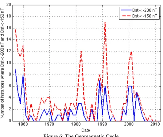
An alternative approach to show the geomagnetic cycle is to plot the annual number of times Dst reaches a specified value. Different values of Dst have been suggested, we chose to specify a value of -150 nT and -200 nT, because generally these values are considered extreme for severe geomagnetic events. Figure 6 shows the number of instances the Dst was less than -200 nT, and less than -150 nT, from 1957 to 2012. The year 1957 is the earliest verified Dst data from World Data Center for Geomagnetism in Kyoto, Japan.

(23)

Figure 6: The Geomagnetic Cycle

The purpose of this plot is to clarify the geomagnetic cycle. As expected, the two scenarios, Dst less than -200 nT and Dst less than -150 nT, follow the same general trends, but with different amplitudes. Interestingly, since 2006 it is the first time zero instances of severe geomagnetic storms have occurred for more than three years. The three-year periods of zero severe geomagnetic storms began in 1964 and 1995. It has currently been six years since the last severe geomagnetic storm of a Dst less than -200 nT.

(24)

CHAPTER 3: DATA FROM INMARSAT

To better understand and mitigate the effects of space weather on the performance of its satellite fleet, Inmarsat, one of the world’s leading providers of global mobile satellite communications services, has partnered with MIT and researchers in the space weather community. This partnership focuses on correlations of space weather with satellite component and system performance, and methods for mitigating potential degradation.

The effects of space weather can greatly inhibit the performance of geostationary communication satellites and their ground stations. However, much work remains to be completed in order to achieve an in-depth understanding of the specific types of space weather events that significantly impact component health, and the necessary methods for mitigating component failures. Understanding the causal relationship between space weather and component health is important because this knowledge will help improve the robustness of satellite hardware and thus improve the services that satellite operators provide to their customers.

Furthermore, the space radiation environment is an important aspect of satellite design that should be accounted for to meet the satellite’s performance and lifetime requirements. Advances in technology have led to a reduction in the size of satellite components – on the micro and nano scales –, which inadvertently has increased their susceptibility to the effects of space weather [Baker, 2000; Wilkinson, 1991; Gubby, 2002]. Electrical upsets, interference, and solar array degradation are just a few of the known effects of the space environment. In fact, as a result of space weather, satellite operators are occasionally forced to manage reduced performance or fully decommission satellites, amounting to social and economic losses of several tens of millions of dollars per year [Baker, 1998]. Therefore, we have conducted a correlation analysis to better understand space weather’s affect on spacecraft that should improve satellite design and reduce the maintenance cost for satellite operators.

In this analysis, more than 500 MB of on-orbit component telemetry and component anomaly data for Inmarsat’s satellite fleet are analyzed. Inmarsat’s telemetry database is used to identify and investigate both nominal and anomalous component performance from 1990 to 2012. Data on solid-state power amplifiers and eclipse durations were analyzed, along with anomaly and SEU information for each satellite. Table 2 describes the collected Inmarsat satellite telemetry.

Table 2: Telemetry Descriptions

Telemetry Parameter Description

SSPA Current Solid-state power amplifier current SSPA Temperature Solid-state power amplifier temperature

Total Bus Power Instantaneous power of the main power bus, power values are calculated from prime and redundant

voltage and current sensors on the main bus Solar Panel North/South

Short Circuit Current

Output of the short-circuit cell current sensor located on the outboard panel of the north and south wing,

used to determine when satellites are in eclipse Solar Panel North/South

(25)

SSPAs are key components for accurately transmitting signals in communication systems, and provide advantageous reliability, ruggedness, size and cost compared to alternatives such as traveling wave tube amplifiers [Sechi, 2009].

The Solid State Power Amplifier (SSPA)

The primary task of solid-state power amplifiers is to increase the power of an input signal to a predefined level. For spacecraft applications, amplifiers are needed because the input communications signal is often degraded due to the atmosphere, through which it must emit to reach the satellite. Therefore, the signal must be amplified, or the power of the signal must increase, to restore the original signal and accurately transmit the signal to the end user. The two most important performance parameters of SSPAs are output power level and power gain The gain of an SSPA, G, is the ratio of the output to input power and is generally measured in decibels, dB [Colantonio, 2009].

SSPAs are non-linear components, yet the device can operate linearly when the amplitude of the input signal is low. As the input signal increases it reaches a level where the output power of the signal saturates [Sechi, 2009]. Amplifiers on communication satellites are generally operated slightly below saturation. The maximum power output with the highest efficiency occurs at the saturation point, however the risk of signal distortion occurs when the input power is beyond the “operating point”. The specific operating point should be optimized for the individual satellite [Elbert, 2002].

(26)

In terns of energy, SSPAs convert DC power into microwave energy power. Efficiency, expressed as a percentage, is the amplifiers ability to convert the DC power into microwave power, and is also referred to as drain efficiency. Ultimately, efficiency determines the power supply of the amplifier. A high efficiency amplifier provides high-transmitted power and increases the overall system performance [Colantonio, 2009].

The European satellite bus manufacturer, EADS Astrium, equips several of their designs with a L-Band SSPA. This 0.75 kg amplifier, shown in Figure 8, is specifically used for mobile communication phased array antennas, which require tight gain and tracking performance with superb Dc/RF conversion efficiency. The SSPAs provide 15 W output power capability. Additional features of this amplifier include 5 degree phase tracking, 0.5 dB gain tracking, peak efficiency of 32%, production rate of 15/week, and spin off products in S and navigation bands. In the past, these amplifiers have flown on several ESA and Inmarsat satellites [Astrium]. Figure 8 shows the EADS Astrium L-Band SSPAs.

Figure 8: EADS Astrium L-Band SSPA with dimensions of 217 mm x 107 mm x 47 mm A satellite anomaly occurs when a component operates outside of its defined threshold for nominal performance. Thresholds are established to monitor the health of components, and notify operators when the component experiences anomalous performance, which limit the operational lifetime of the satellite. For SSPAs, the main threshold of concern is the amplifier current. The SSPA current determines the amplification capability of the device. When the amplifier is irradiated the semiconductor material (such as silicon or Gallium Arsenide) is affected by surface charging, deep dielectric charging from relativistic electrons, or impact from high energy more massive particles such as protons. Over an undetermined period of time, this results in a change in conductivity of the material and thus leads to a change in current, which is a parameter monitored and tracked in housekeeping telemetry. If the current exceeds the upper threshold the SSPA will saturate, and if the current exceeds the lower threshold the SSPA will not provide enough current to adequately amplify the signal. Therefore the effects of space weather can cause the amplifiers to operate insufficiently and even cause amplifier anomalies.

Traffic Analysis of SSPA Currents

Over the course of a spacecraft’s lifetime, component health and performance degrades as a result of exposure to space weather [Baker, 2000]. These anomalies are often assumed to result from the taxing launch environment and maneuvers that a satellite experiences within the first two years of operation. Anomalies that occur within the first two years of operation can pose challenges when analyzing the source of anomaly, as correlations between anomalies and space weather events may be confused with anomalies from the launch environment. Thus, it suggests

(27)

that space weather should be monitored as a cause of anomaly at all stages or the spacecraft’s life.

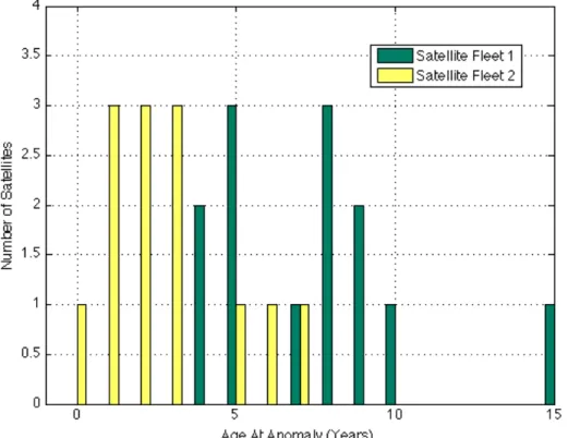
Figure 9 shows the age, or number of years after launch, of the satellites when an SSPA anomaly occurred. The age has been approximated to the closest whole year, so 4.6 years is recorded as 5 years. For the second satellite fleet, most anomalies are shown to occur in the first two years of operation. Anomalies that occur during the first two years of a satellite’s life are sometimes due to the extreme conditions that the sensors experience during launch and during the maneuvers to reach the allocated orbital slot. However, it is possible that these anomalies are not “burn-in” or transition effects but could be due to harsh space weather events. Seven of the twenty-six anomalies occurred in the first two years of the satellites lifetime, and 6/7 anomalies occurred within two weeks of a severe radiation space weather event caused from relativistic electrons. Inmarsat satellites have an expected lifetime of fifteen years. One can expect that as the satellite increases in age the likelihood of anomalies should also increase. Nonetheless, there is not an obvious increase in Figure 9 because the two co-plotted fleets consist of satellites at different points in their expected lifetime. While the satellites in the first fleet are up to fifteen years old, the satellites in the second fleet are at most six years old.

Figure 9: Satellite Age at time of SSPA Anomaly including anomalies that occur within two years of launch [Lohmeyer, 2012]. The two different color bars, yellow and green, designate two

different satellite fleets.

The eight Inmarsat satellites considered in this analysis have each experienced between zero and eight SSPA anomalies. These anomalies have occurred as early as in first three months of operation and as late as at nearly fifteen years of operation. Figure 9 shows that at age 1, 2, 3, 5,

(28)

and 8 years after launch the same number of anomalies occur (3 each). We again note that the satellite fleets have different designs and SSPA configurations.

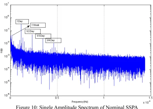
Nominal SSPA currents over the lifetime of each satellite have inherent periodicities as a result of traffic, or customers using Inmarsat’s communication services. Figure 10 is the single amplitude spectrum for a nominal SSPA. As depicted, the most prevalent periodicities are one week, one day, a half of a day, a third of a day and a quarter of a day.

Figure 10: Single Amplitude Spectrum of Nominal SSPA

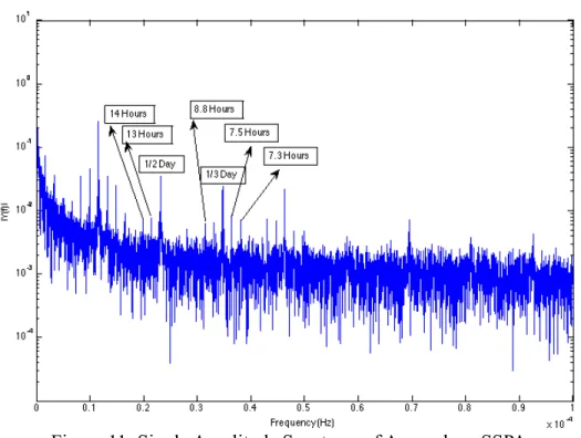
We observed some cases where the frequency spectrum of an anomalous SSPA showed periodicities in addition to those shown for a nominal SSPA in Figure 10. In the nominal case, we expect periodicities to be related to traffic and the diurnal cycle. Figure 11 shows an example of the single amplitude spectrum of an anomalous SSPA, where periodicities of 1 day, 1 week, half of a day, one third of a day and a fourth of a day are clearly present, in addition to higher power clusters of harmonics.

(29)

Figure 11: Single Amplitude Spectrum of Anomalous SSPA

The periodicities on a larger scale, such as months, imply that seasonal trends exist. Seasonal trends suggest that that the SSPA data is dependent on solar activity, and motivates the investigation of relationships between anomalies and eclipse seasons, as well as anomalies and space weather in a more general sense.

Correlation of Anomalies and SEUs with the Eclipse Seasons

The Earth’s orbit, while not truly circular, revolves around the Sun along the ecliptic plane, which is 23.5 degrees from the Earth’s rotational axis. Regardless of the year, the Earth’s rotational axis maintains this orientation and pointing direction. As a result of the rotational tilt angle and the Earth’s rotation about the Sun, seasons occur, making longer periods of daylight in the summer and shorter periods of daylight in the winter. As the satellites approach autumn and spring, they enter equinox, which is approximately 21 days long. In the initial days of equinox the eclipse duration, or amount of time the sunlight is blocked, last for ~ 1-2 minutes, yet when the Sun reaches equinox the duration of eclipse can increase up to 72 minutes [Intelsat, 2012]. Generally, geostationary satellites have a direct view of the sun and are able to utilize energy from the solar panels as a power source. However, during an eclipse the Earth blocks sunlight from reaching the solar arrays and forces the satellite operators to monitor and control power management during the known eclipse seasons.

(30)

Figure 12: Eclipse Seasons [CNES, 1979]

In this work, the start and end dates of eclipse season as well as the longest eclipse duration times for the four satellites with the highest traffic levels were tracked. The Inmarsat recorded eclipse dates are displayed in Table 3, and are slightly longer than the eclipse periods denoted by the red arrow in Figure 12. To simplify the table, instead of listing the annual range, the earliest eclipse start date since 1996, and the latest eclipse end date are listed. The period in the center of the eclipse season where the longest eclipse durations occur does not exceed ten days. For example the longest eclipse start and longest eclipse end for Satellite W occur from March 16-24, a period of nine days.

Table 3: Summary of Eclipse Durations Satellite Spring Season Start Spring Season End Longest Eclipse Start Longest Eclipse End Fall Season Start Fall Season End Longest Eclipse Start Longest Eclipse End W Feb.

25 April 15 March 16 March 24 Aug. 30 Oct. 19 Sept. 21 Sept. 26

X Feb. 26 April 19 March 16 March 24 Aug. 30

Oct. 20 Sept. 21 Sept. 26

Y Feb. 26 April 18 March 22 March 26 Aug. 30

Z Feb. 26 April 20 March 21 March 27 Aug. 30

Lunar eclipses require a less intensive procedure because they only occur once or twice a year, and do not produce significant discharges. Regardless, in the event of a lunar eclipse operators

(31)

instruct the satellites to enter eclipse mode because the onboard propagators do not track the moon’s location.

The two eclipse seasons are from late February to mid-April and late August to late October; the longest eclipses generally last between 68 to 73 minutes [Lohmeyer, 2012]. The eclipse seasons coincide with the vernal and autumnal equinox, because during equinox the Earth blocks the Sun’s light from reaching the satellites. Interestingly, the SSPAs are not primarily found to occur during equinox, but occur more so in the two solstice periods.

Table 4 shows the season in which each of the twenty-six SSPA anomalies occur. The specific satellite longitudes are kept anonymous to protect competitive advantage. Interestingly, the majority of the SSPA anomalies does not occur during the eclipse seasons, but instead occur between November and January, during the northern winter solstice. The northern equinoxes coincide with the fewest number of SSPA anomalies. Based on these data, it appears that the geometry of the Earth eclipsing the sun in addition to the measures taken by the operators during eclipse seasons for power management seem to reduce the number of SSPA anomalies. As shown in Table 4, ten and seven anomalies occur over solstice periods, compared with three and six anomalies in periods of eclipse.

Table 4: The number of SSPA anomalies that occur during different seasons Satellite Nov. – Jan.

Solstice Feb. – April Equinox May – July Solstice Aug. – Oct. Equinox A 1 0 0 1 B 3 0 3 0 C 2 1 1 1 D 2 0 0 0 E 0 0 1 0 F 1 2 1 4 G 1 0 1 0 Total 10 3 7 6

During these two eclipse seasons, satellite operators pay particular attention to monitor and control power management of the satellites as the Earth blocks the sunlight from reaching the solar panels [Lohmeyer, 2012]. ESD is found to occur during rapid changes in potential associated with the beginning and end of the eclipse seasons [Fennel, 2001]. Based on this data, it appears that the additional measures taken during eclipse seasons to protect the satellite components also reduce the number of SSPA anomalies, as ten and seven anomalies occur in periods of solstice, and three and six anomalies occur in periods of eclipse. It should also be noted that solstice periods, which coincide with spring and fall, are also when geomagnetic activity is most active [Rangarajan and Lyemori, 1997].

For the SEU and eclipse analysis, the four satellites with the highest traffic were considered. Of these four satellites, two have advanced computing systems that consist of primary and secondary computers that are each susceptible to SEUs. Table 5 shows the distribution of SEUs over separate quarters of the year. However, when comparing the occurrence of SEUs with the different of eclipse seasons, no obvious correlation exists.

(32)

Table 5: Eclipse and SEU Satellite Nov. – Jan.

Solstice Feb. – April Equinox May – July Solstice Aug. – Oct. Equinox W 2 0 2 3 X 2 4 1 2 Y primary 2 3 3 8 Y secondary 7 11 14 13 Z primary 11 12 10 8 Z secondary 12 12 7 5 TOTAL 36 42 37 39

(33)

SSPA Anomalies and Satellite Local Time

Choi et al. [2012] found that for 95 publicly available GEO anomalies the majority of the anomalies occur mainly between midnight to and dawn in local time. However, the anomalies were not specific to only SSPAs but also include a variety of failures including electrostatic discharge and power outage. In Figure 13, we plot the local time of each of the 26 SSPA anomalies on the eight Inmarsat satellites. In future work, we will consider the temporal distribution of anomalies and their relationship to different types of charging. For example, anomalies associated with internal charging should be equally distributed in MLT, whereas surface charging should preferentially occur in the midnight to dawn sector.

Figure 13: Satellite Local Time1 for the twenty-six SSPA anomalies. The radial distance from the center of the plot shows the number of anomalies that occurred, as at local midnight, when four

(15%) SSPA anomalies occurred.

The 26 SSPA anomalies we have, from two different fleets, may not be sufficient to draw clear conclusions on time dependence, although they are all from the same type of component failure. However, we will summarize their current distribution. Nine (35%) occur between midnight and 06:00 local time. This is the largest distribution of anomalies compared to three other six-hour periods (midnight – 06:00, 06:00 – noon, noon – 18:00, 18:00 – midnight). Seven of 26, or 27%, occur between 06:00 and local noon, as well as seven between local noon and 18:00. Lastly, four of the 26 SSPA anomalies occur between 18:00 and local midnight (not including midnight). It is interesting that numerous studies, e.g. Choi et al. [2012], Wilkinson [1994], and Fennel et al. [2001], suggest that satellite anomalies depend on satellite local time. However, a majority of

(34)

these anomalies may be associated with surface charging, and further investigation into the SSPA anomaly mechanism is needed to provide context.

(35)

CHAPTER 4: SPACE WEATHER DATA

For historical space weather information, the primary databases included in this study are: NOAA Geostationary Operational Environmental Satellites, the Geomagnetic Equatorial Dst Data Service in Kyoto, Japan, the Royal Observatory of Belgium’s Solar Influences Data Analysis Center and the Advanced Composition Explorer Satellite.

Geostationary Operational Environment Satellites (GOES) Data

To obtain dates for severe solar storm events (X-rays), radiation storm events (SEPs and relativistic electrons), and additional data on the space environment during times of anomalous satellite component activity, the authors used the NOAA National Geophysical Data Center to obtain GOES Space Environment Monitor (SEM) data. This sensor suite has provided continuous magnetometer, particle and X-ray data since the mid-1970s, and is a primary source for public, military and commercial space weather warnings [GOES, 1996].

Table 6 shows the GOES satellites that have been active from 1996 – present. GOES 11 was not included due to technical difficulties and GOES 9 and GOES 15 were not used because of their short coverage time span.

Table 6: GOES Satellite Initial and Final Coverage Times GOES Satellite Initial Coverage Time Final Coverage Time

GOES 8 Jan. 1995 June 2003

GOES 9 April 1996 July 1998

GOES 10 July 1998 Dec. 2009

GOES 11 July 2000 Feb. 2011

GOES 12 Jan. 2003 Aug. 2010

GOES 13 April 2010 Sept. 2012

GOES 14 Dec. 2009 Present (comes and goes)

GOES 15 Sept. 2010 Present

At any point between 1996 and 2012 at least two of the GOES 8 – GOES 15 satellites were collecting data. During this time, several of the GOES satellites were either decommissioned into a parking orbit or experienced technological difficulties and are thus not included in this study. Nonetheless, of the remaining GOES satellites, GOES 12 is the primary satellite used for gathering SEM data, GOES 8, 10, 13 and GOES 14 were also used when one of these satellites was located closer to the anomalous satellite and for dates outside of the and GOES 12 coverage time span.

The SEM consists of three magnetometers, an X-ray/extreme ultraviolet sensor (XRS/EUV), and an energetic particle sensor/high-energy proton and alpha detector (EPS/HEPAD). This study focuses on telemetry from the EPS/HEPAD, which measures the aforementioned particle flux throughout the magnetosphere. Specifically, the instrument consists of two energetic proton, electron and alpha detectors (EPEADs), a magnetospheric proton detector (MAGPD), a magnetospheric electron detector (MAGED), and a HEPAD [NSWPC, 2007].

For this research, the GOES EPS 2 MeV electron flux channel in five-second intervals data is used to assess relativistic electrons at the time of SSPA anomalies. Additionally, the GOES EPS