Automobile valve manufacturing : technical and econoimc analysis

Automobile Valve Manufacturing

Technical and Economic Analysis

by

Luis David German

Licenciado en Ciencias Fisicas Universidad de Buenos Aires, 1992

SUBMITTED TO THE DEPARTMENT OF MATERIALS SCIENCE AND ENGINEERING IN PARTIAL FULFILLMENT OF THE REQUIREMENTS OF THE DEGREE OF

MASTER OF SCIENCE IN MATERIALS ENGINEERING AT THE

MASSACHUSETTS INSTITUTE OF TECHNOLOGY

AUGUST 1996

C 1996 Massachusetts Institute of Technology. All rights reserved.

Signature of Author:

_,epartment

Certified by:

Joel P. Clark Professor of Materials Engineering . Thesis Supervisor

Accepted by:.

rF T;:I

Linn W. Hobbs Professor of Materials Science Chairman, Department Committee on Graduate Studies

SEP 2

71996

~c~Y~ ~

V

Automobile Valve Manufacturing

Technical and Economic Analysis

by

Luis David German

Submitted to the Department of Materials Science and Engineering on August 23, 1996 in Partial Fulfillment of the

Requirements of the Degree of Master of Science in Materials Engineering

ABSTRACT

As a consequence of increased rates of new product introduction, rapid technology changes and global competition, consumers around the world have a broader product menu from which to choose. To compete effectively, companies must continually work to improve quality, productivity and flexibility.

Flexible manufacturing systems, FMS, are often cited as the means to achieve both flexibility and productivity. However, this is not the only route possible. Flexible manufacturing can also be achieved by means of process selection. Choosing an appropriate process can lead to the desired flexibility without the high levels of investment usually needed to implement a FMS.

This paper presents the case of the Argentinean engine valve industry, in which companies achieved the needed flexibility through process selection. To demonstrate this, the paper presents a cost based definition of manufacturing flexibility and a methodology for measuring it.

While there are many types of flexibility, this paper is strictly concerned with issues related to the variability of demand and its effect on manufacturing cost. Flexibility is defined as the marginal cost of changes in demand variables. Two different demand scenarios are analyzed, one involving changes in the product mix, and another involving changes in overall product demand.

The use of a cost based definition of flexibility requires the ability to estimate manufacturing costs as a function of the product demand variables. This is accomplished through the use of technical cost modeling (TCM). TCM breaks down the manufacturing process into its different cost elements and estimates each one separately based on basic engineering and physics principles. Clearly defined economic and accounting principles are applied to arrive at a final cost breakdown for the process. This gives the model the ability to estimate costs for a range of inputs and thus it can be used to analyze the effects of changes in the demand variables.

The methodology is demonstrated using the example of engine valves producers in Argentina. The worldwide market for engine valves is dominated by two competitors, which only focus on

large production volume parts. Consequently, their production processes are geared towards large lot sizes. By focusing on smaller production volumes and customized parts, two Argentinean companies have filled a void in the market. To accomplish this, these companies had to acquire flexibility, but without large investments, due to a lack of capital. This paper demonstrates that despite their limited capital, the Argentinean valve producers were able to develop a more flexible manufacturing system through the selection of an appropriate technology thereby achieved their strategic goal of capturing a niche market.

Thesis Supervisor: Joel P. Clark

TABLE OF CONTENTS

Acknow ledgm ents ... 8

1. Introduction ... 9

1.1. The need of Flexibility... 9

1.2. Types of Flexibility... 11

2. O utput Flexibility through Process Selection... 14

2.1. Achieving Flexibility... 14

2.2. Cost Based Definition of Output Flexibility... 14

3. Cost Estim ation... 18

3.1. Technical Cost M odeling Review ... ... 18

3.2. Computation of the Cost Elements Used in TCM ... 21

3.2.1. M aterials Cost... 21

3.2.2. Direct Labor Cost... 21

3.2.3. Energy Cost... 22

3.2.4. M ain M achine Cost... 22

3.2.5. Auxiliary Equipment Cost... 23

3.2.6. Tooling Cost... 23

3.2.7. M aintenance Cost... 23

3.2.8. Overhead Cost... 24

3.2.9. Building Cost... 24

4. Case of Argentina Valve M anufacturers ... ... 27

4.1. Introduction ... 27

4.2. Global Valve Industry... 27

4.3. The Argentinean Engine Valve Industry... 27

4.4. Process Choices... 31

4.4.1. The Forging Process... ... 31

4.4.2. The Forge-extrusion Process... 32

4.5. Process Selection/The need for Flexibility... 33

4.6. Cost Estimation for The Valve M aking Processes... 37

5. Conclusions ... ... 45

Appendix 1: Valve M anufacturing Cost M odel... 46

LIST OF FIGURES

Figure Page

Figure 1: The Hayes-Wheelwright Product/Process Matrix ... 10

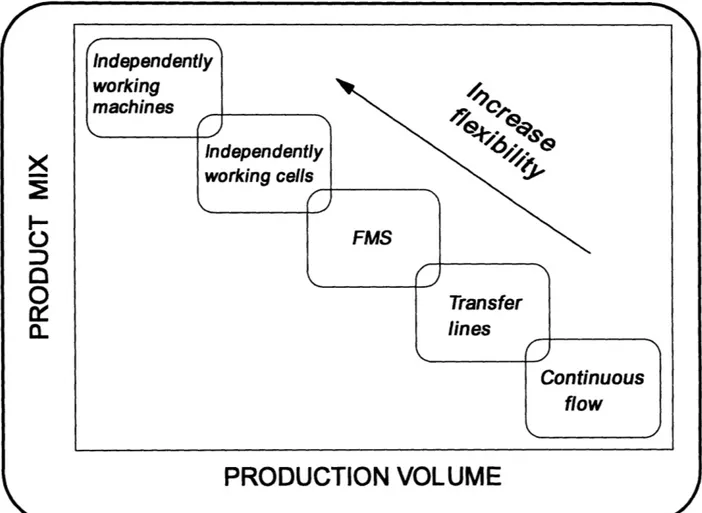
Figure 2: Typical production systems in a production volume -product mix space... 12

Figure 3: Cost comparison of two processes as a function ofproduction volume... 16

Figure 4: M odel lay out... 25

Figure 5: Argentinean automobile production over the last two decades... . 29

Figure 6: USA. automobile production over the last decade... 30

Figure 7: A schematic of the forging step used in the 'forging" process... 34

Figure 8: Processes steps involved in manufacturing a valve using the "forging" and the 'forge-extrusion" process technologies... 35

Figure 9: Schematic of the forming step of the 'forge-extrusion" process... 36

Figure 10: Cost breakdown for producing a valve using the 'forging" process... 38

Figure 11: Cost breakdown for producing a valve using the 'forge-extrusion" process ... 39

Figure 12: Manufacturing cost sensitivity to production volume and lot size for the 'forging" process... 40

Figure 13: Manufacturing cost sensitivity to production volume and lot size for the 'forge-extrusion" process... 41

Figure 14: Regions of dominant cost-effectiveness for the two competing processes... 43

Figure 15: Cost break down by process steps, material cost, and set up for producing a valve using the two competing processes... . 44

LIST OF TABLES

Page

Table 1: The "rules of thumb "for manufacturing cost estimate... Table 2: Cost elements used in TCMfor both variable and fixed cost.... ...

ACKNOWLEDGMENTS

To all these people I owe different aspects of my great experience at MIT.

In first place, to Professor Joel Clark for giving me the opportunity to work at MSL, for his academic advice and help throughout these first two years at MIT, for his generous financial assistance, and for his warm friendship.

To Professor Don Lessard for letting me be part of the "Mendoza team" and for his help and trust during this first year of the CIT project.

To Rich Roth with whom I spent excellent moments working on and discussing about the project, for his assistance in finishing this thesis and for having helped making a working trip a very

enjoyable experience.

To Dr. Frank Field for always finding the time to answer whatever question I had, and to the rest of the MSL, Maja, Elicia, Sam, Anil, Randy, and Jay for making the experience of forming part of this group a great one.

To the members of the "Mendoza team", Alex, Carolina, Horacio and Omar for being very "gauchos."

To my friends, Cari, Adro, Marce, Jerry, Ale, Daniel, Marcela, and Pampa for there friendship, support, and advice, for long hours of interesting conversation, testy "asados", rainy camping experiences, and long trips. To my friends Sally, Zohar, Yair, and Yoel for the same reasons seasoned with a "tzabra" flavor.

To my family, Bube, Celia, Mario, Doty, Arielo, Rorro, and Li for there continuous support and love that remains strong no matter the physical distance.

To my lovely wife, Adri, who helped me, supported me and comforted me even when MIT managed to get on my nerves. Without her unconditional support, I would not have managed to get to this point.

1. INTRODUCTION

1.1. THE NEED OF FLEXIBILITY

Flexible manufacturing along with quality and productivity has become a key issue in manufac-turing operations. More and more manufacturers have realized that these three factors are keeping their companies competitive in a rapidly changing global market.

Increased competition has meant a large increase in the number of products being offered to the consumer. In many industries, customized products are now common. To produce large product lines without a substantial cost penalty, manufacturing flexibility is required. This need is further enhanced by the rapid changes in the state of technology. Flexible systems are more easily able to accommodate new technologies and thus take advantage of recent advances.

Two major classifications of manufacturing processes are relevant when discussing the flexibility of the system, batch and continuous flow processes. Batch processes involve the flow parts through the process steps in groups, while continuous processes consist of parts flowing through in an uninterrupted sequence. Although traditional mass production techniques using transfer lines or continuous flow operations are cost effective for large volumes of parts, they are not very flexible. Alternatively, a job-shop or batch flow environment (usually requiring a higher labor component) organized in cells is far more flexible, but less productive. Clearly there is a trade-off between productivity and flexibility. One way of visualizing this situation was introduced by'] _and

is shown on figure 1.

The use of flexible manufacturing systems, FMS, may be a suitable compromise for some

manufacturers[2]_{. FMS usually involves the implementation of high levels of automation to achieve}

r

Low volume

High product

mix

PRODUCT

MIX

_Do-

High volume

_{Low product}

mix

Loosely linked

process steps

CO

C/)

w

0

a.

Highly linked process

steps. Continuous

automated and rigid flow

V

Figure 1: The Hayes-Wheelwright Product/Process Matrix

dp- ft% __j ,Wft woooll

/00

k

j

done under what is commonly termed CIM, computer integrated manufacturingf31. The final objective is to be able to efficiently manufacture batches composed of only a minimum number of parts by reducing to the overall cycle time. Cycle time reductions are achieved through a reduc-tion in the set-up times required to change from one product to another. Although FMS and CIM are very efficient ways of achieving flexibility, their implementation requires high levels of capital investment compared to the job-shop organizationE4]_{. Figure 2 shows how FMS fits into the}

overall manufacturing spectrum of product mix and product volume51_.

1.2. TYPES OF FLEXIBILITY

Generally speaking flexibility is the ability of a system to adapt to changes in the environment. In the past, several authors have attempted to define flexibility from a manufacturing perspective6E_'7_'1

It is clear form their works that there is not a unique definition. An approach followed byl9_'

analyzes flexibility under five categories corresponding to five different sources of variability that a manufacturer may have to face.

Demand Variability: May arise in two forms. Volume variability linked to market demand volatility, and changes in product mix which may occur over time.

Supply Variability: Deals with volatility in the manufacturing inputs such as the quality, volume and delivery time of incoming material.

Product Variability: Includes everything from the introduction of new products to daily changes in product design.

Process Variability: Comes in two general forms. Changes in process technologies and changes in managerial technologies.

Figure 2: Typical production systems in a

Workforce andEquipment Variability: Includes uncertainties due to labor turnover, absenteeism, equipment reliability, etc.

Different industries are affected by these types of variability in different ways. Some face high product variability, like the computer industry, for which the rate of introduction of new products has been steadily growing over the last two decades. Others have to deal with supply variability. For example some food processing industries are faced with seasonal changes in their supply of raw materials. In some cases, the main source of variability comes from the demand side. An example of this is the engine valve industry, especially in relatively small automotive markets where the demand for the total number of valves and the different types of valves varies from year to year.

As alluded to above, demand variability comes in two types, volume variability and product mix variability. The ability of an industry to respond to changes in both of these types of demand variability is called output flexibility"1_.

2. OUTPUT FLEXIBILITY THROUGH

PROCESS SELECTION

2.1. ACHIEVING FLEXIBILITY

The required output flexibility can be achieved either through conventional means, such as

increased investment in automation, or through the choice of a manufacturing process which more easily lends itself to changes in the input variables. It is well documented that different processes have different cycle and setup times. Even more, they have different economies of scale, even when used to manufacture the same product. Therefore choosing a suitable technology to achieve output flexibility is a problem that deserves special consideration.

The need for output flexibility is not only affected by the demand variability but also by issues internal to the firm. These considerations typically center on the strategic intent of the firm. For example, a firm whose focus is only on large production volume products is likely to face little product mix variability and therefore have less need for output flexibility than the firm which is targeting many small production volume parts.

Once the need for output flexibility is determined, the next step is to make decisions concerning features central to the manufacturing operation, such as capacity, process technology and management technology to name a few. Above all, an appropriate manufacturing process, one which is inherently flexible, must be selected.

This approach is contrary to the standard thought that automation is the preferred route towards reaching flexibility. Investing in automation usually implies moving towards a capital intensive operation which may not be cost effective in all situations. Flexibility can also be achieved by selecting a manufacturing process which by its very nature has shorter setup and changeover

times. In this way flexibility is reached without the need for additional automation and the

Selection of a manufacturing process is not only dependent on the need for flexibility and the strategic intent of the firm, but also on the available technologies. In some cases, manufacturing processes for a given part can vary substantially, while in other cases the choices are less striking. For example the production of doped semiconductor wafers can be done either by ion implanta-tion or by thermal diffusion, two completely distinct process technologies. In other cases, there is only one appropriate technology, but numerous variations. For example, the production of many forged products can by accomplished with expensive dies and little need for additional finishing operations, or with less expensive dies, but additional process steps.

2.2. COST BASED DEFINITION OF OUTPUT FLEXIBILITY

As previously discussed, flexibility is defined as the relative effect of given parameters (e.g. production volume, lot size) on the overall cost. A flexible system would then be the one that can operate under different conditions without having a significant impact on its cost. The most flexible system at a given production volume would be the one with the lowest change in cost per change in the input variables. In the case of output flexibility, the input variables are the demand volume and the product mix. Output flexibility can be visualized by the slope of the curves in Figure 3. For any given process, it is assumed not only that cost decreases monotonically with increasing production volume, but also that the slope of this curve is monotonically decreasing (strictly within the range of the capacity of the line). Therefore, the process which is more cost effective at lower production volumes, i.e. the process with the lower fixed costs, must have a greater degree of output flexibility for all production volumes within its range of applicability.

0

Fixed Cost

Fixed Cost A

Variable Cost A

Variable Cost B

Production Volume

Figure 3: Cost comparison of two processes as afunction ofproduction volume

L

-L

\11'.ý

11. - I

In general, the goal of the firm is to produce parts in the most cost effective manner. If one could predict exactly the production volume or required lost sizes, the choice of the process technology would be straightforward. However, near the point at which the two processes yield the same part cost, PV*, process flexibility may become a determining factor. For production volumes less than PV*, process A is both more cost effective and more flexible and thus the clear choice. At produc-tion volumes greater than the maximum possible when using process A, PVAm, process B must be chosen. However, at intermediate production volumes, those lying between PV* and PVAm, the choice is less clear. Process A offers flexibility, but at a cost. These production volumes regions are summarized below.

if PV < PV* : Process A is both more cost effective and more flexible if

PV

: Process B is the only possibility

if PV* < PV < PVAx

:

In the last case choosing between processes A and B will depend on the value the firm places on flexibility and the degree of variability one expects to encounter, since the demand variability can easily move the actual PV the region below PV'.

3. COST ESTIMATION

3.1. TECHNICAL COST MODELING REVIEW

As both volume and product mix flexibility have been defined in terms of cost, determination of these flexibilities comes down to the ability to estimate manufacturing costs over a range of inputs. While many cost estimation techniques exist, few offer significant depth of analysis or the ability to investigate the effects of changes in input variables on the manufacturing cost. The technical cost modeling (TCM) technique overcomes these disadvantagest 1 2'1 3'4"151.

The traditional approach to estimate manufacturing cost has always been based on "rules of thumb" and accounting empiricism. These rules include factors which lead to oversimplification and other specific weaknesses. Important issues such as processing variables, production volume, part geometry, etc. do not play any role on such a simplistic approach. Even more, the part cost is extremely sensitive to some assumed factors such as machine rent, even though machine rent does not factor in important effects like economies of scale, part geometry, and others. Examples of these traditional "rule of thumb" cost estimates are presented in Table 1.

Rule Name Part Cost ($/unit) =

Multiplier Multiplier Factor x Material Cost Rent Material Cost + (Cycle Time x Machine Rent) Burden (Material Cost + Labor Cost) x Burden Rate

These approaches lack the key ingredient necessary for analyzing the flexibility of the manufac-turing process, the ability understand the dependence of the output (cost) on changes in the input parameters, such as production volume, lot sizes, etc.

On the contrary, TCM is specifically designed to investigate the interactions between process variables and cost. TCM breaks down the different cost elements and estimates each one

separately. This is done from basic engineering and physics principles of each of the manufac-turing processes involved in the overall operation. Clearly defined economic and accounting principles are then applied to these cost elements. These elements are then classified as either fixed or variable costs.

The division of cost elements into variable and fixed categories is a widely accepted accounting and engineering classification[61 _{. The basic difference is that variable cost is a function of the}

annual production volume while fixed costs are not. The elements used under these categories are:

Table 2: Cost elements used in TCMfor both variable and fixed cost

Central to the goals of TCM has been the development of a tool for analyzing the manufacturing cost implications of different manufacturing strategies, business conditions and materials selection. This methodology has been used to evaluate not only the competitive implications of conventional materials and materials forming technologies, but also developmental and research alternatives,

Variable Cost Fixed Cost

Material Main Machine

Direct Labor Auxiliary Equipment

Energy Tooling

Maintenance Overhead

quantifying the strengths and weaknesses of these alternatives as well as pinpointing the critical factors (both engineering and economic) which contribute to this competitive position. TCM is designed to work with so-called "zero-stage" design data, making it possible to take advantage of this information in the critical early phases of product and process development. This is particu-larly important since the firm's strategic intent must be decided prior to the selection of an appropriate process technology.

In an early stage of a process design, TCM can be used to specifically analyze the effect of changes in production volume and lot size (product mix) on the overall cost. This cost response can then be interpreted as the ability of the system to adjust to demand and product variabilities. A definition for output flexibility can then be presented in terms of the TCM output.

Several interesting scenarios can be analyzed in this way. A first analysis could look at the effects of changes in both the production volume and lot size independently. However, it is rare that these variables are actually independent. Smaller production volumes generally result in smaller lots sizes. One can hold the ratio of the production volume to the lot size fixed and analyze the effect of changes in just one input on the overall cost. By examining the case where the lot size equals the production volume, one assumes the extreme condition of manufacturing a specific product just once during the entire year, and is representative of the process flexibility with respect to product mix only.

Another set of analyses can be conducted under the assumption that the production line is dedicated to a single part. In this case fluctuations in the production volume lead to idle times. TCM can be used to estimate the part costs at varying levels of production to determine the

volume flexibility of the process.

Both mix and volume flexibility are needed to understand the overall implication of having a broad

3.2. COMPUTATION OF THE COST ELEMENT USED IN TCM.

Table 2 presents the nine different cost elements, divided in two categories used in developing technical cost models. The next sections present a brief explanation of how each of these elements are calculated in the models.

3.2.1. MATERIAL COST

The cost of material can be estimated directly from the design of the piece and the price of the raw material, but the part design weight may not always be an accurate measure of the total amount of material used. An accurate treatment of the amount of material to be used should include scrap losses of downstream steps. Further, it should be kept in mind that in many cases the listed material market price may be different from the actual transaction price. It is not possible to capture such differences in a model given that they involve managerial decisions and different transfer scenarios.

3.2.2. DIRECT LABOR COST

Direct labor cost reflects the number of man-hours required to produce a given part. It is a function of the wages paid, the time required to produce the part, the number of workers needed for the process, labor productivity and the total amount of operating hours per year. The hourly wage should represent the cost of a worker-hour to the company, not the salary perceived by the worker.

3.2.3. ENERGY COST

Ideally, the energy cost can be calculated by using a detailed energy balance for each process and the cost of the energy source. However, this is extremely complex since it involves all possible energy losses, energy efficiencies and considerations of heat, mass and momentum transfer. Because in most cases the cost of energy is a small portion of the total piece cost, it is reasonable to estimate it as a function of the equipment energy consumption per hour. Only in some proce-sses, such as heat treatment, does the cost of the energy merit treatment in greater detail.

3.2.4. MAIN MACHINE COST

The cost of the machine is in most cases a function of the equipment capacity and the degree of automation. The equipment capacity can be related to a large number of design parameters. Knowing the design parameters and therefore the required equipment capacity the machinery cost

can be obtained from vendors.

For a given level of investment in equipment, an annual cost must be derived. It is assumed that the investments are paid for by loans over the estimated period of life of the equipment at a

prede-termined interest rate. The annual payment, R, is calculated using the standard amortization equation given bellow.

R=P (I +i)fi

[(I

+ i) - 1

Where i is the interest rate, N is the number of periods (years) over its life, P is the total investment.

The next step is to distribute the cost over the production volume to obtain a cost per piece base. If the equipment is dedicated to the manufacturing of a particular part, the annual cost is then divided by the total production volume to obtain the per piece cost. Otherwise, the annual cost of

the equipment is allocated to the parts by the ratio of the time required to finish the work over the total annually available time.

3.2.5. AUXILIARY EQUIPMENT COST

Typically auxiliary equipment for material fabrication include compressors, storage equipment, conveyors, etc. A simpler way of estimating auxiliary equipment cost assumes that the ratio of the auxiliary equipment to the main machine is constant. For many fabrication processes this

assumption is good enough to yield valid results.

3.2.6. TOOLING COST

Calculating a tooling cost per part can be very complicated. Estimating both the investment in a set of tooling and the number of parts it will produce during its life span is very difficult. It would involve variables such as the material, design and size of the part, the automation level, the tool quality, and processing variables such as speed. Further, tools can be dedicated like a set of forging dies or non-dedicated like inserts for a lathe.

A simple method for estimating tooling cost would involve regression analysis. Historical tooling data is collected and analyzed to evaluate correlation between input data and tooling life and investment.

3.2.7. MAINTENANCE COST

Maintenance cost is difficult to quantify precisely. There are two types of maintenance, scheduled and unscheduled. Unscheduled maintenance is done in response to problems as they develop. An accurate estimation of the occurrence of problems requires prediction of probabilistic events.

Instead, a simple calculation is done by estimating maintenance cost as a fix percentage of

machinery cost and building cost.

3.2.8. OVERHEAD COST

Overhead accounts for laborers and other costs not directly involved in the manufacturing.

Nonetheless these elements are necessary in the production process. This group include personnel

working in supervisory, managerial, janitorial, security, and accounting positions. The overhead

cost is usually classified as a fixed cost and can be estimated as a fixed percentage of the total

capital investment.

3.2.9. BUILDING COST

The cost of building space is relatively straightforward to estimate, given the amount of space

required and the price per surface unit. The space required is determined by the quantity and size

of the equipment which must be installed. The price per surface area can be obtained from real

estate agents or industry sources. Once the data has been obtained and the investment established

it can be distributed over the entire production volume using the allocation method explained on

section 3.2.4.

3.3. THE COST MODEL LAYOUT

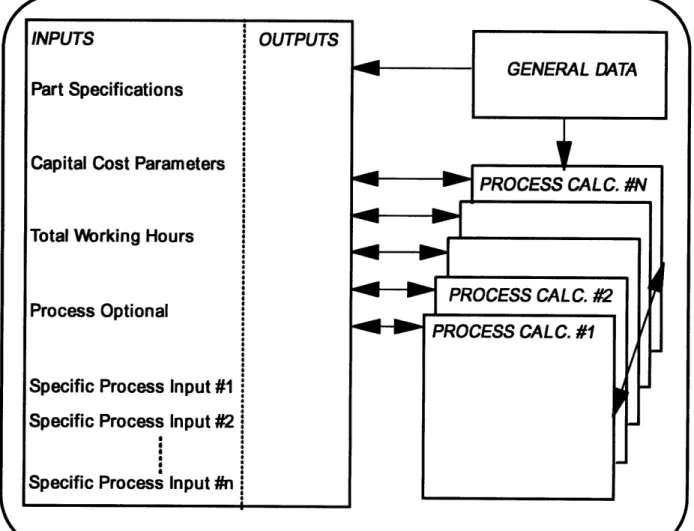
The manufacturing model itself is built using Lotus 1-2-3 spreadsheet. A typical layout is shown

in figure 4. The model is divided into three sections: input/output, general data and processes

calculations. The appendix 1 present a view of all these different sections for the valve

manufac-turing model.

Figure 4: Model Layout. 25

..,0000/

The input/output section is divided in two parts. The first one for the inputs, and the second one for the outputs. The input part has three columns. The first one called "Default" or "Estimated" includes general model values. These values were chosen based on industry standards, general information, and calculations performed by the model. All the values assumed in the first column can be overridden according to the user needs. The third column indicates the final values that are going to be used for the simulation. These inputs are divided into several categories which are:

-Part Specifications, in which general data is entered regarding valve geometry, materials, and production volume.

-Capital Cost Parameters, in which general data for capital cost analysis is entered.

- Total Working Hours, based on standard values for the industry.

-Process Optional is used to select the subset of processes which will be involved in the overall manufacturing operation.

-Specific Process Inputs, consists of different inputs for each of the individual processes involved in the manufacturing operation. Process specific inputs such as "Cycle time", "Labor require-ment", "Main machine cost", are entered here. An "On/Off' flag indicates whether or not any particular process is being taken into account in the overall model calculations.

The output shows a breakdown of the cost by process step and cost elements such as fixed and variables costs, as described previously in this chapter.

The general data section includes data such as energy cost, material properties, processes characteristics, etc. that is going to be used throughout the model.

Finally, under the processes calculations section individual cost estimations are made for each of the process steps used in the overall manufacturing operation.

4. CASE OFARGENTINA VALVE MANUFACTURERS

4.1. INTRODUCTION

The Argentinean engine valve industry provides an excellent example of the use of an appropriate manufacturing process to yield the flexibility needed to achieve the strategic goals of the firm. By employing a processing technique that has shorter set up times and lower fixed costs, the Argenti-nean valve makers are able to compete on the basis of cost in the market for lower volume engine valves.

4.2. GLOBAL VALVE INDUSTRY

The worldwide engine valve industry is dominated by two competitors who control approximately 90% of the more than 1 billion units per year global market. They target high volume products and use the substantial economies of scale to compete on the basis of cost. In order to be cost competitive, they organized manufacturing lines based on operating in the region defined as "transfer line" in the figure 2.

The remaining 10% represents a substantial market, but consists of a large variety of low volume products which are difficult to produce in a cost effective manner using the mass production techniques of the two main producers. This market consists of engine valves for motorcycles, buses, planes, off-shore boats, grass trimmers, pumps and specialty automobiles, such as race cars. Staying competitive requires the ability to produce low volume or custom made parts in relatively small lots. Success is determined mainly by the manufacturer's ability to cope with variability in demand (both volume and product mix) by achieving output flexibility.

4.3. THE ARGENTINEAN ENGINE VALVE INDUSTRY

The Argentinean engine valve manufacturers have had a history of competing in a very similar environment. These companies started operations during the mid 1950's under a protected local market as a supplier to the Argentinean motor vehicle assemblers. As indicated in figure 5, the Argentinean automotive industry has experienced a very high level of volatility over the last two decadestm.

This volatility situation, with oscillations from 100,000 units/year up to 400,000 units/year and the low overall demand made them target Argentina's after market as well. By doing this, they expec-ted to slightly stabilize the fluctuations in the automakers' demand. Nevertheless, Argentina's after market was particularly complicated due to the large product mix resulting from the long average vehicle life of nearly 20 years.

This is considerably different than the large, relatively stable market faced by the two large global competitor. Despite the difficulties experienced in the American automobile market over the last past 10 to 20 years, it represent a far more stable situation than the experienced in Argentina for the same period. Figure 6 shows that the automobile production in the USA over the last decade '81 _{lhas fluctuated only in the range of 45M units/year up to 53M units/year.}

To survive in this highly volatile market, these companies had to be flexible enough to accommo-date wide swings in orders from year to year. Their difficulties were further compounded by a fluctuating macroeconomic situation. This meant there was little access to the capital needed to acquire flexibility through the purchase of expensive automation equipment.

Instead they were forced to find an alternate solution. This came in the form a more suitable manufacturing process. Instead of operating in the region defined as "transfer lines" in figure 2, they used the "forge-extrusion" process which allowed them to organize the production around the idea of "independent working cells". In this way they gained output flexibility simply by using

~--- ---- N

Millon Units

*o 30

₀

S20

0

E

10

0

85' 86' 87' 88' 89' 90' 91' 92' 93' 94'

95'

El

CarsM Trucks

Year

a

Figure 6: USA. automobile production over the last decade

\41'..

..,0/

a process which was tailored to the production of smaller lots and volumes. While they saved the cost of expensive automation equipment, they sacrificed the ability to compete on cost when producing large volumes. This was an appropriate tradeoffgiven the highly volatile, low volume market situation facing the Argentinean manufacturers.

In the last few years, the opening of Argentina's economy and the MercoSur market integration expanded the operation horizon of this companies, giving them the ability to export to other markets. Their initial strategic choice and the associated selection of a process technology, have given these companies a cost advantage in the niche market of low volumes and customized products.

4.4. PROCESS CHOICES

The selection of a suitable manufacturing process was central both to the early success of the Argentinean valve manufacturers in their closed domestic market and to their competitiveness in the low volume niche of the global market. Valve production can be accomplished by two

techniques, "forging" and "forge-extrusion". The Argentinean producers chose the use of the low volume, highly flexible process of forge-extrusion instead of attempting to take advantage of the economies of scale of the forging process.

4.4.1. THE FORGING PROCESS

The high volume producers typically use a process known as "forging"'i91 _{to produce valves. The}

forging process requires a large investment in equipment and tooling, but has short cycles times and low variable costs, and is typically associated with high volume producersl20]_{. Its main}

drawback is that the set up times for changing from one product to another can be quite

high level of capital investment means that large production volumes are essential in order to recover the fixed costs.

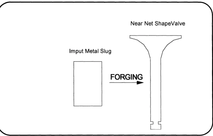
The forging process is based on plastically deforming a material cylinder into a near net shape part. A schematic of this is given in figure 7. In addition to the forging step, other processes are required to produce the final part. Figure 8 contains a flow chart for the process typically used to produce engine valves.

The forging process is a very efficient method for manufacturing high production volumes. Companies which are able to target the major automakers and thus benefit from economies of scale can achieve a significant cost advantage by using this process. However, this cost advantage is entirely dependent on the economies of scale of the process. As a result, there is a considerable

cost penalty associated with the use of the forging process when producing smaller volumes or smaller lots of valves.

4.4.2. THE FORGE-EXTRUSION PROCESS

The forge-extrusion process is similar to forging in that they are both essentially forging methods. However, the forge-extrusion process involves plastic deformation only to the valve head. In turn the equipment requirements are less stringent and thus the capital investment is smaller. However, this savings does not come without a price. The forge-extrusion method results in a part which is much farther from the desired final geometry of the valve, and thus more extensive machining is needed. A schematic of the forge-extrusion process is shown in figure 9. As for the forging

process, other processes are required to produce the final part. These processes are essentially the same ones presented in figure 8 for the forging case. The main difference is on the amount of work required by each of these processes. After the forge-extrusion process step, the part is less

closer to the final valve dimensions than the part obtained after the forging process step.

Therefore the amount of material to be removed after the forge-extrucion step is far larger than the amount of material to be removed after the forging step.

As in the forging process, the forge-extrusion process also requires additional steps to achieve the final part shape and tolerances. These are very similar to those presented in the figure 6. The major difference is that in this case, a larger amount of material must be removed after the forge-extrusion step compared to the amount of material removed after the forging step in the previous process.

Since more material is removed in the "after-forming" steps, the forming itself is less critical to the final quality. Thus, the forge-extrusion step can be done with less expensive equipment and

tooling. Even more, the set-up time for this process is greatly reduced. While the final steps like machining and grinding are more critical and have a longer cycle time than in the forging process, they can be reduced through the introduction of computer numerical control (CNC) systems, thus improving the flexibility.

The short set up times and lower capital investment means that the forge-extrusion process is far better suited to producing smaller lots. This gives the process more flexibility with regard to both product mix and total production volume. Larger mixes can be used to mitigate the effects of volume fluctuations in a single product line. Furthermore, the lower investment means that idle time is less expensive and thus demand variations do not impose as great a cost penalty. These features are significant if the manufacturer operates in a market with a high degree of demand variability.

4.5. PROCESS SELECTION/THE NEED FOR FLEXIBILITY

The selection of the more cost effective manufacturing process is clear for most anticipated market conditions. (Low volumes/high product mix should be produced using the forge-extrusion process while high volumes/low product mix is best produced using the forging process).

However, at production volumes for which both processes yield similar costs, the choice is less obvious. As previously stated, figure 3 indicates that in a region between PV* and PVAM~, there is a tradeoffbetween cost and flexibility.

N

Near Net ShapeValve

Imput Metal Slug

Fill A

Figure 7: A schematic of the forging step used in the 'forging" process

FORGING

_No

Figure 8: Processes steps involved in manufacturing a valve using the

Input rod

Valve

HEAD

MELTING,

(TRUSION

Figure 9: Schematic of the forming step of the "forge-extrusion" process

/I

r

4.6. COST ESTIMATION FOR THE VALVE MAKING PROCESSES

The determination of the optimal process selection is dependent on an understanding of the production volume at which the two processes are cost competitive and the cost response to changes in production volume near this point. To accomplish this, technical cost models were developed for the two manufacturing processes, forging and forge-extrusion, including all additional steps necessary to produce the final part.

For the purpose of comparing these two processes, costs were estimated for a generic intake valve for a mid size automobile engine. This valve has a simple design made out of standard HNV3 steel[21

]. TCM was used to estimate the overall manufacturing cost using each process. A

cost breakdown for each process is given in figures 10 and 11 for the case of a production volume of 300,000 and lot size of 75,000 valves.

There are three major differences between these processes. First, the forge-extrusion option has a larger labor component, 30% compared to only 16% for the forging case. Even more, if the labor requirement is compared by its man/hour component, that is, if the differences in wages between Argentina and USA are eliminated, the forge-extrusion process will have nearly eight times the labor component of the forging process. Second, machinery and tooling represent a smaller fraction of the total cost of forge-extrusion than forging (20% compared to 30%). This reflects the fact the forge-extrusion process is less capital intensive. The third difference is the material cost. The rods of steel needed in the forge-extrusion process are more expensive than those used in the forging process.

The cost models were also used to observe the sensitivity of the manufacturing cost to variations in the production volume and lot size. Results, in the form of three dimensional graphs are presented in figures 12 and 13. Each graph shows the per piece cost as a function of the production volume and lot size.

I"

Figure 10: Cost break down for producing a valve using the "forging" process.

--f

r

L m

ICost

Break Down

/

r

f

$10,000 $1,000 $100

Cost ($)

_$10

Figure 12: Manufacturing cost sensitivity to production volume

and lot size for the 'forging" process.

I, ~1111111111111~11111~1111111~111~1111~ / r 1 i

$10,000 $1,000 $100

Cost ($)

Figure 13: Manufacturing cost sensitivity to production volume

and lot size for the "forge-extrusion" process.

/

r

Lot Size

It is evident from these graphs that the cost associated with forging process exhibits a stronger dependence on the demand variables. According to the definition stated at the beginning of this paper, the forging process has less output flexibility.

A comparison of the two techniques can be seen by analyzing the intersection of the two surfaces shown in figures 12 and 13. This defines two feasible regions in the "Lot Size-Production

Volume" space (it is unfeasible to have lot sizes greater than the annual production volume). Each region is characterized by the more cost effective process for that particular set of inputs and is shown in figure 14.

Figure 14 indicates that the forging process yields a lower manufacturing cost in the region where production volumes are larger than approximately 300,000 valves per year and lot sizes are larger than approximately 75,000 valves. For the rest of the "Lot Size-Production Volume" space the

cost effective choice is the forge-extrusion process. This overall behavior is mainly due to the much smaller set up time needed to run the forge-extrusion process. Only when the production volume is large enough to diminish the relative cost effect of the set up time, does the forging

process becomes the choice.

Near the boundary between the processes the overall manufacturing costs are similar. Neverthe-less, the set up time of the forge-extrusion process is still much smaller than the set up cost of the forging process. On the other hand, the manufacturing cost (excluding set up) of the forge-extrusion process is still higher at this point. This is presented in figure 15, where it can be seen that the cost due to set up is approximately 10 cents for a valve made by the forging process compared to only 2 cents for one produced by the forge-extrusion process. This was calculated using a production volume of 300,000 and a lot size 75,000 and corresponds to the region around PV* in figure 3. Relatively small uncertainties in the demand variables could lead to a change in the selection of the optimal process. Consequently, it is especially important to understand the demand variability near this boundary.

10,000,000

1,000,000

100,000

10,000

1,000

100

10

1

1100

10

_1,000

10,000

1,000,000

100,000

10,000,000

Production Volume

Figure 14: Regions of dominant cost-effectiveness for the two competing processes

4)

V

\S",-

j

Cost

($)

C

2

Seat grinding Inspection & Packaging

N Forge-Extrusion * Forging

Figure 15: Cost break down by process steps, material cost, and set up

for producing a valve using the two competing processes.

0

Ipi

-I

_I

_I

ELM

V

A

I

5. CONCLUSIONS

A cost based methodology can be used to determine the flexibility of competing manufacturing processes. Under conditions where manufacturing costs are similar, flexibility may be a key factor in selecting the most appropriate process technology. This is particularly true if demand variability is likely to be substantial. Such is the case when choosing a process for making intermediate volumes of engine valves, especially in developing economies where demand variability can be extremely high. The selection of the optimal process therefore must consider these effects, and take into account the additional value of the flexibility of the system.

The Argentinean engine valve makers are able to capture the niche market represented by small and intermediate volume valves by employing a more flexible processing technique. By taking advantage of the shorter setup times and lower capital investments associated with the

APPENDIX 1

VALVE MANUFACTURING COST MODEL

Part Specifications

Capital Cost Parameters

What process do you use? (1= forging or 0= extrusion) Is it a bimetalic valve? (1 = yes or 0 = no)I

1 01

1 0

Total Working Hours

Process Optional

I

SO, -"1110, M,

N SM.

*ý

21=ý=

F

vlxelm

MINIMUM'

I.-IMIL 1.3

AMR=

[am FMM

21M, -M-0

PER , 1ý

M.,

-M-1,

M.

IF"

0-111ý

IN

Im",

Mix. EM law

NOW

00

Emig=

Specific Process Inputs

ECS.

-

-si

N

Q

,...

...

M....d

a

e

...

{ s .

..

...

.. ..

...

..

% u t n

..

.

..

...

.

..

...

..

..

...

.

..

...

..

..

....

..

...

..

IMF

uemn peo m

...

"4tycme44(W

...

%o

...

n

..

Tea...

ob

.r

...

...

...

...

..

set~.

a.

...

m~~~~e.

...

r

4 t ot

-

-

-

--

-

-

-

-

--

-

-

-

-

-

-

!11:!:

Xp

l

General Data

Natural gas : 36.6 MJ/m^3

Processes Calculations

CUTTING ON

Number of parts (output) 253,387

Number of parts (input) 253,641 Cycle time (sec) 5

Effective time to produce a part (sec) 7 Number of lines 0.08

... i::ii:i::...:$ ::i .• : ..:: ...:i::•:•l .g • .•

... .. ... ... • ... •. ~i ...... .::::::::::::::::: ... : . ... .... .... .... .... .. . . .. . .

IA

L

..

...

y

ar p rcen

....

...

b

o

...

2

$2960

9101

...

E

C...e..p

rc nt nv st en

...

....

...

...

...

.o

...

...

..

...

s

.,

0

4

Total~~~~~

1

...

1330

B99

Tota Pa

s

4C

...

3.2

..

.0...

BIBLIOGRAPHY

1. R. H. Hayes and S. C. Wheelwright, "Restoring Our Competitive Edge: Competing Through Manufacturing," John Wiley & Sons, NY. 1984, p.2 0 8-2 2 3.

2. D. J. Parrish, "Flexible Manufacturing," Butterworht-Heinemann Ltd, London, 1990, p.2 1. 3. M. Mesina, W. J. Bartz, E. Wippler, "CIMHandbook," Butterworth-Heinemann Ltd.,

London, 1993.

4. C. H. Fine, "New Manufacturing Technologies," Strategic Manufacturing, Dow Jones-Irwin, Illinois, 1990.

5. P. G. Ranky, "Flexible Manufacturing Cells and Systems in CIM," CIMware Limited, England, 1990, p.14.

6. D. Gerwin, "The Do's and Don'ts of Computerize Manufacturing," Harvard Business

Review 60, Vol. 2, March 1982, p.107-116.

7. J. A. Buzacott, "The Fundamental Principles of Flexibility in Manufacturing Systems,"

Proceedings of the First International Conference on Flexible Manufacturing Systems, UK, 1982,.

8. J. Browne, "Classification of Flexible Manufacturing Systems," The FMSMagazine, April

1984, p.114-117.

9. S. L. Beckman, "Manufacturing Flexibility: The Next Source of competitive Advantage,"

Strategic Manufacturing, Dow Jones-Irwin, Illinois, 1990, p.10 7-13 2.

10. A. Fiegenbaum and A. Karnani, "Output Flexibility-A Competitive Advantage for Small Firms," Strategic Management Journal, Vol. 12, 1991, p.101-114.

11. B. Poggiali, "Production Cost Modeling: A Spreadsheet Methodology," SM. Thesis, Dept. Mat. Sc. & Eng.., MIT., September 1985.

12. N. V. Nallicheri, "A technical and Economic Analysis of Alternate Net Shape Processes in Metal Fabrication," Ph.D. Thesis, Dept. Mat. Sc. & Eng., MIT., June 1990.

13. J. E. Neely, "The Commercial Potential for Advanced ceramics Produced by low Pressure Injection Molding," SM. Thesis, Dept. Mat. Sc. & Eng.., MIT., February 1992.

14. H. N. Han, "The Competitive Position of Alternative Automotive Materials," Ph.D. Thesis, Dept. Mat. Sc. & Eng., NUMIT., May 1994.

15. R. Roth, "Materials Substitution in Aircraft Gas Turbine engine Applications," Ph.D. Thesis, Dept. Mat. Sc. & Eng., MIT., February 1992.

16. E. R. Sims, "Precision Manufacturing Costing," Marcel Dekker Inc., New York, 1995. 17. ADEFA, Annual Report, various years.

18. "The 100 Year Almanac," Automotive News, Vol. 1, April 1996.

19. S. Kalpakjian, "Manufacturing Processes for Engineering Materials," Addison-Wesley Publishing Company, USA, 1992.

20. K. C. Ludema, R. M. Caddell, A. G. Atkins, "Manufacturing Engineering: Economics and Processes," Prentice-Hall Inc., New Jersey, 1987.

21. J. M. Larson, L. F. Jenkins, S. L. Narasimhan, J. E. Belmore, "Engine Valves-Design and Materials Evolution," Journal of Engineering for Gas Turbines Power, Vol. 109,