HAL Id: hal-01573653
https://hal.archives-ouvertes.fr/hal-01573653
Submitted on 10 Aug 2017HAL is a multi-disciplinary open access archive for the deposit and dissemination of sci-entific research documents, whether they are pub-lished or not. The documents may come from teaching and research institutions in France or abroad, or from public or private research centers.
L’archive ouverte pluridisciplinaire HAL, est destinée au dépôt et à la diffusion de documents scientifiques de niveau recherche, publiés ou non, émanant des établissements d’enseignement et de recherche français ou étrangers, des laboratoires publics ou privés.
at watershed scale in crystalline aquifers
Benoît Dewandel, Yvan Caballero, Jérôme Perrin, Alexandre Boisson, Fabrice
Dazin, Sylvain Ferrant, Subash Chandra, Jean-Christophe Maréchal
To cite this version:
Benoît Dewandel, Yvan Caballero, Jérôme Perrin, Alexandre Boisson, Fabrice Dazin, et al.. A method-ology for regionalizing 3-D effective porosity at watershed scale in crystalline aquifers. Hydrological Processes, Wiley, 2017, pp.2277 - 2295. �10.1002/hyp.11187�. �hal-01573653�
1
A methodology for regionalizing 3-D effective porosity at watershed scale in
1crystalline aquifers
2Benoît Dewandel1*, Yvan Caballero1, Jérôme Perrin2, Alexandre Boisson2, Fabrice Dazin3,
3
Sylvain Ferrant4, Subash Chandra5 & Jean-Christophe Maréchal1
4
1- BRGM, D3E/NRE Unit, 1039 rue de Pinville, 34000 Montpellier, France,
5
b.dewandel@brgm.fr
6
2- BRGM, D3E/GDR Unit, 3 Av. C. Guillemin, 45100 Orléans, France,
7
3- SIRS, 27 rue du Carrousel, Parc de la Cimaise, 59 650 Villeneuve d’Ascq, France,
8
4- CNRS; GET, 14 Avenue Edouard Belin 31400 Toulouse, France,
9
5- Indo-French Centre for Groundwater Research, CSIR-NGRI, Uppal Road, Hyderabad
10
500606,Telangana State, India.
11
* Corresponding author
12
Abstract
13An innovative approach for regionalizing the 3-D effective-porosity field is presented and
14
applied to two large, overexploited and deeply weathered crystalline aquifers located in
15
southern India. The method derives from earlier work on regionalizing a 2-D
effective-16
porosity field in that part of an aquifer where the water table fluctuates, which is now
17
extended over the entire aquifer using a 3-D approach. A method based on geological and
18
geophysical surveys has also been developed for mapping the weathering profile layers
19
(saprolite and fractured layers). The method for regionalizing 3-D effective porosity
20
combines: water-table fluctuation and groundwater budget techniques at various cell sizes
21
with the use of satellite based data (for groundwater abstraction), the structure of the
22
weathering profile and geostatistical techniques. The approach is presented in detail for the
23
Kudaliar watershed (983 km2), and tested on the 730 km2 Anantapur watershed. At watershed
24
scale, the effective porosity of the aquifer ranges from 0.5% to 2% in Kudaliar and between
25
0.3% and 1% in Anantapur, which agrees with earlier works. Results show that: i) depending
26
on the geology and on the structure of the weathering profile, the vertical distribution of
27
effective porosity can be very different, and that the fractured layers in crystalline aquifers are
28
not necessarily characterized by a rapid decrease in effective porosity; and ii) that the lateral
29
variations in effective porosity can be larger than the vertical ones. These variations suggest
30
that within a same weathering profile the density of open fractures and/or degree of
31
weathering in the fractured zone may significantly varies from a place to another.
32
The proposed method provides information on the spatial distribution of effective porosity
33
which is of prime interest in terms of flux and contaminant transport in crystalline aquifers.
34
Implications for mapping groundwater storage and scarcity are also discussed, which should
35
help in improving groundwater resource management strategies.
36 37
Key words: Effective porosity, regionalization of aquifer parameters, upscaling, hard-rock
38
aquifer, crystalline aquifer
39 40
2
1. Introduction
41
Among the most important data for groundwater management or for reliable hydrogeological
42
modelling, are accurate estimates of the spatial variation of hydrogeological properties,
43
especially effective porosity and hydraulic conductivity. Data on spatial- and depth-variations
44
of the effective porosity are important issues for contaminant transport, and particularly —as
45
combined with the aquifer geometry—they provide an accurate image of the groundwater
46
storage of an aquifer, thus valuable information for groundwater management issues.
47
In crystalline (granite and metamorphic rocks) aquifers, the regionalization of
48
hydrogeological properties (i.e. estimating their spatial distribution) is further complicated,
49
because of their strong natural heterogeneity. Various degrees of fracturing and connection
50
between fracture networks induce strong variations of hydrogeological properties at all scales
51
(e.g., Paillet, 1998; Maréchal et al., 2004; Le Borgne et al., 2004, 2006). The few available
52
works on upscaling and regionalizing aquifer parameters in crystalline aquifers has mainly
53
focused on transmissivity or hydraulic conductivity mapping, based on hydraulic-test data
54
(Razack and Lasm, 2006; Chandra et al., 2008), classified transmissivity (indexed) maps, or
55
potential aquifer-zone maps (Krásný, 1993, 2000; Lachassagne et al., 2001; Darko and
56
Krásný, 2007; Madrucci et al., 2008; Dhakate, et al., 2008; Courtois et al., 2010).
57
Over the past three decades, the geological and hydrogeological characterization of
58
crystalline aquifers has seen significant improvements (Chilton and Foster, 1995; Taylor and
59
Howard, 2000; Lachassagne et al., 2011, 2015; Wyns et al., 2004, Maréchal et al., 2004;
60
Dewandel et al., 2006; Ayraud et al., 2008; Guiléneuf et al., 2014; Roques et al., 2014a).
61
These works show that, where such hard-rocks are exposed to deep weathering processes, the
62
geometry and hydrodynamical properties of aquifers are closely related to the weathering
63
grade of the parent rock. In granite-type rocks, including gneiss, a typical weathering profile
64
comprises two main stratiform layers sub-parallel to the paleo-surface at the time of
65
weathering processes (e.g. Wyns et al., 1999 and 2004, Krásný and Sharp, 2007; Maréchal et
66
al., 2007, Reddy et al., 2009, Lachassagne et al., 2011, etc.). From top to bottom they are: (i)
67
the saprolite layer, a sandy-clayey to clayey-sandy material usually characterized by low
68
hydraulic conductivity and high effective porosity; (ii) the fractured layer, characterized by a
69
depth decrease in the number of fractures (Houston and Lewis, 1998; Howard et al., 1992;
70
Maréchal et al., 2004; Wyns et al., 2004; Dewandel et al., 2006) and usually low effective
71
porosity. The underlying unfractured and fresh bedrock is only locally permeable and most
72
authors consider that hydraulic conductivity is related to local tectonic fractures with highly
73
variable hydrodynamic properties (e.g., Pickens et al., 1987; Leveinen et al., 1998; Walker et
74
al., 2001; Kuusela et al., 2003).
75
Based on this concept of a stratiform hard-rock aquifer, Dewandel et al. (2012) proposed
76
a methodology for regionalizing effective porosity- and also hydraulic conductivity- at the
77
watershed scale. The method is based on the concept that large-scale variations in hydraulic
78
head may characterize large-scale properties. For the effective porosity, the method
79
combines—at cell scale—water-table fluctuation and groundwater-budget techniques in the
80
absence of recharge from rainfall, an aggregation method, and variogram based statistics and
81
kriging techniques to allow a relevant mapping. The approach was tested on an unconfined
82
granitic aquifer exposed to deep weathering, located in South India (Maheshwaram
83
watershed, 53 km2). The resulting estimates were confirmed by hydraulic tests carried out on
84
the area and by effective-porosity estimates at watershed scale (Maréchal et al., 2004, 2006;
85
Dewandel et al., 2006, 2010). However, the developed method could only determine effective
3
porosity values for that part of the aquifer where the water table fluctuates, but not for the
87
entire aquifer.
88
The novelty of the present work consists in using satellite based data (for groundwater
89
abstraction) and in developing an original approach that allows extending the effective
90
porosity in 3-D to the entire aquifer while combining it with the structure of the weathering
91
profile. A method for mapping the weathered layers (based on geological and geophysical
92
surveys) is also developed.
93
Results are illustrated in detail for the Kudaliar 983 km2 unconfined granite aquifer exposed
94
to deep weathering in southern India, State of Telangana (Fig. 1a). The method then was
95
tested on another area with a more complex geology, the Anantapur watershed (730 km2,
96
State of Andhra Pradesh, India; Fig. 1b), but this area suffers from a lack of available
97
observations, especially concerning geology. Both watersheds are overexploited (CGWB,
98
2009). The main results are presented in the discussion and compared to the ones of Kudaliar.
99
The method for regionalizing 3-D effective-porosity field data requires knowledge of the
100
lateral and vertical variations of the weathering-profile (saprolite and fractured zone) on a
101
hectometric to kilometric scale, as well as spatial estimates of groundwater abstraction and
102
seasonal water-level measurements. This study provides additional information of the spatial
103
heterogeneity of effective-porosity values at catchment scale and with depth, which are rare
104
information. The implications for mapping groundwater storage and scarcity in term of
105
groundwater management issues are discussed as well.
106 107 108 109 110 111
2. Field data
1122.1 Location and climate
113
The Kudaliar catchment (983 km2) lies 50 km north of Hyderabad in the Telangana region of
114
Medak District, India (Fig. 1a). The area has a relatively flat topography with elevations
115
ranging from 430 to 640 m above mean sea level and the absence of perennial streams.
116
The region has a semi-arid climate controlled by monsoon periodicity. The rainy season
117
(Khariff) occurs from June to October and the dry season (Rabi) from November to May.
118
Mean annual precipitation is about 880 mm, of which about 90% falls during the rainy season.
119
The mean annual temperature is 26°C, but in summer (March to May) it can reach 45°C. The
120
area is rural and populated by about 303,000 inhabitants (Indian Census, 2001; Aulong et al.,
121 2012). 122 123 2.2 Geology 124
4
The geology of the area is relatively homogeneous and consists of Archean biotite granite
125
commonly found in the Hyderabad region (Fig. 1a, GSI, 2002). Locally, the granite is
126
intruded by small pegmatite bodies (1- to 10-metre-wide veins striking N45-60), metre-wide
127
dolerite dykes of several geological ages (2.5–1.6 Ga; GSI, 2002; striking N000, N045,
128
N100), and a few other intrusives (adamellite-granodiorite and amphibolite-hornblende-biotite
129
schist enclaves). The granite is affected by deep in-situ weathering resulting from multiphase
130
weathering-erosion processes (Dewandel et al., 2006). The weathering profile is formed of
131
two main layers: saprolite and a fractured layer. The saprolite layer is composed of a few
132
metres of saprolite of sandy texture (sandy regolith) and a thick layer of laminated saprolite,
133
characterized by an unusual network of preserved sub-horizontal and sub-vertical fractures
134
partially filled by clay. Deeper down, fractured granite, where weathered granite and some
135
clay partially fill decametre-wide sub-horizontal and sub-vertical fractures, constitutes the
136
bottom layer of the weathering profile. This layer is tapped by bore wells for crop irrigation
137
and domestic water supply (mean bore-well depth: 50-70 m). Below the fissured fractured
138
layer, the granite is not fractured and is not considered as an aquifer (Maréchal et al., 2006;
139
Dewandel, 2006, 2012).
140 141
2.3 Groundwater and irrigation
142
As in most of southern India, groundwater is the only perennial water resource and is
143
exploited by a large number of private bore wells (7,000 to 10,000 in the area) for the
144
irrigation of rice, vegetables (tomatoes, eggplant, lady’s finger, chillies, etc.), maize, cotton,
145
and a few other crops (sugar cane, pulses and oilseeds). Plots are watered using flooding and
146
ray irrigation techniques. Well-discharge rates are generally low, ranging from less than
147
1 m3/h to, exceptionally, a few tens of m3/h.
148
Land-use characterization at parcel scale was performed on LISS-4 and Spot-5 images (6
149
and 10 m spacing, respectively) for the 2009 rainy season and the following 2010 dry season,
150
with training and validating ground data (Ferrant et al., 2014). During the 2010 dry season,
151
7.2% of the area was irrigated for rice, 6.8% for vegetables, 1.9% for maize, and 2.1% for
152
other crops (Table 1). It results that about 18% of the entire watershed surface was used for
153
irrigated crops. The remaining ground is covered by built-up areas, pasture, forest,
agro-154
forestry and barren rocky land (boulder area). During the 2010 rainy season, the total
155
cultivated land covered 45% of the watershed and was mainly dominated by cotton (19%;
156
only 3% irrigated, Table 1), maize (15%; 7% irrigated) and rice (10%, all irrigated). Field
157
observations on crop cultivation and irrigation were conducted with farmers to get data on
158
cropping calendars and stages, as well as on watering techniques. Crop watering, determined
159
by bore-well flow rates in the irrigated area, varies from 9 to 12 mm/day according to crops
160
and seasons. These results are similar to those measured on the Maheshwaram watershed
161
located 90 km farther south (Dewandel et al., 2008). Groundwater also supplies domestic
162
uses, which amount is based on census data (Census, 2001). Combined with land-use, such
163
data on groundwater consumption allow computing the seasonal groundwater abstraction on
164
the watershed (Table 1), which was about 121 mm during the 2010 dry season (or 120 Mm3)
165
and about 88 mm for the 2009 rainy season (or 87 Mm3). These results are consistent with
166
those found for the Maheshwaram watershed with its similar cropping pattern: 100±27 mm
167
and 73±9 mm during the dry and rainy seasons, respectively (average over 2002-2005;
168
Maréchal et al., 2006; Dewandel et al., 2010). These computations also show that 86% of the
169
annual groundwater abstraction is used for rice irrigation (196 mm/year; 176 Mm3/year),
170
whereas domestic use is less than 1.5%.
5
Water-table maps were drawn based on groundwater-level measurements from 104 bore
172
wells (abandoned wells, i.e. never pumped) after the rainy season (November 2009, Fig. 2a)
173
and at the end of the dry season (June 2010). Water levels are deep (20 m below ground level
174
on average; Fig. 2b), mainly within the fractured layer, more or less parallel to the
175
topographic surface, and are impacted by the pumping wells.
176 177 178 179 180 181
3. Methods
1823.1. Mapping the weathered layers
183
Because establishing the geometry of the two main weathered layers (saprolite and fractured
184
layers) is the first step of the method, layer-thickness investigations based on geological
185
observations on outcrops and geophysical measurements were carried out.
186
Geological observations consisted in evaluating the saprolite thickness from dug wells.
187
These very large wells (>20 m2), often deeper than 15 m and now dry because of receding
188
water levels, are the only available exposures of the weathering profile. Generally, the deepest
189
ones crosscut the top of the fractured layer, easily recognizable due to the presence of
190
fractured granite at the bottom. About 250 dug wells were identified, 230 of which were
191
suitable for identifying the top of the fractured layer. Other geological observations defined
192
the lithology and identified the area without saprolite cover (the ‘Boulder Area’, i.e. barren
193
rocky area corresponding to outcrops of the fractured layer). The locations of geological
194
observations are presented in the ‘results section’ (see Fig. 5a).
195
Geophysical measurements consisted in electrical resistivity logging carried out in
196
abandoned bore wells for estimating the layer thicknesses of the weathering profile. The
197
logging tool, a simple probe designed at the Indo-French Centre for Groundwater Research
198
(IFCGR, Hyderabad), is composed of two active electrodes (i.e. current and potential) fixed
199
at 1 m separation on the probe and two additional electrodes (current and potential) kept on
200
the ground at a relatively infinite distance from the bore well. The probe was connected to a
201
“SYSCAL Switch (Junior)” resistivity meter and used to log at every 0.5 m intervals in the
202
saturated zone. True resistivity could not be computed because of lack of data on bore-well
203
diameter and on water electrical conductivity. However, previous experiments carried out in
204
the same granite with the same weathering profile (Maheshwaram watershed, 90 km from
205
Kudaliar; Chandra et al., 2009, and the Choutuppal experimental hydrogeological park at
206
100 km; Chandra et al., 2015) showed very small differences between apparent and true
207
resistivity of the rock, and a very good consistency between the weathered-layer thicknesses
208
estimated from resistivity logs and detailed bore-well geological logs. Thus, the apparent
209
resistivity has been taken for estimating layer thicknesses of the weathering profile.
210
Measurements were carried out on 39 bore wells in the Kudaliar watershed. Figure 3 shows an
211
example of resistivity well logging where weathering profile layers are recognized.
212 213
6
3.2. Regionalizing 3-D effective porosity
214
3.2.1. Effective porosity for the zone where the water table fluctuates (2-D approach)
215
Dewandel et al. (2012) developed an approach for estimating the effective porosity field for
216
that zone of the aquifer where the water table fluctuates. It consists in combining the
water-217
table-fluctuation method and groundwater budget for a dry season (i.e. without groundwater
218
recharge) with an aggregation method implying computations at various cell sizes. Assuming
219
negligible recharge, the change in groundwater storage of an unconfined aquifer during a dry
220
period is (Schicht and Walton, 1961; Maréchal et al., 2006; Zaidi et al., 2007):
221
s=Sy*h=ET+Q-RF+qoff-qon+qbf (1)
222
where s is the change in groundwater storage (m), h is the water-table fluctuation (m), Sy
223
is the effective porosity (or aquifer specific yield) of the zone where the water table fluctuates
224
(unit less), ET is the evaporation from the water table (m), Q is the abstraction of groundwater
225
by pumping (well-discharge rate) (m), RF is the irrigation return flow (m), qon and qoff are
226
groundwater flow in and out of the aquifer (m), and qbf is groundwater base flow to streams
227
and springs (m).
228
Groundwater abstraction by pumping, Q, has been computed from the land-use map. The
229
map has been aggregated on a 100x100 m cell grid, each cell corresponding to a specific
230
cropping pattern and/or urban area. Knowing the groundwater consumption of each land-use
231
category, the groundwater abstraction map could be computed (Fig. 2a). Irrigation return
232
flow, RF, was calculated according to return flow coefficients of each groundwater use (ratio
233
of water input over return flow to the aquifer); Table 2 gives the used return-flow coefficients
234
(Maréchal et al., 2006; Dewandel et al., 2008). Each coefficient was thus applied to the
235
corresponding groundwater use for the dry season, which allows computing the net
236
groundwater abstraction Q-RF in each cell.
237
Some terms of Eq. (1) can be neglected. Due to deep water levels in the area, on average
238
20 m in 2009-2010 (Fig. 2b), ET is a very small component of the budget, typically less than
239
1 mm/y (Dewandel et al., 2010) and can be neglected. In addition, the absence of perennial
240
stream- and spring flow because of the disconnection between the water table and the
241
hydrological network, leads to nil qbf. Therefore, Eq. (1) can be simplified, and Sy becomes:
242
Sy=(Q-RF+qoff-qon)/h (2)
243
Maréchal et al. (2006) and Dewandel et al. (2010) used Eq.2 for estimating Sy at the
244
watershed scale for the part of the aquifer where the water table fluctuates. At this scale and
245
because water table is a subdued replica of the topography, qoff and qon were low-values and
246
thus their balance could be neglected (qoff-qon ~0). Assuming a small size affected by pumping
247
with known Q-RF and h values, qoff and qon or their balance will not be negligible as the
248
radius of influence of the pumping will be larger than the size of the cell. Therefore assuming
249
for this example a nil qoff-qon will induce an overestimation of Sy in Eq.2. Conversely, if the
250
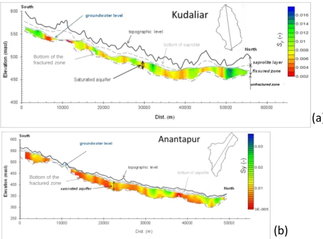
cell size is larger than the radius of influence of the pumping, or a group of pumping wells,
251
the whole of the pumped volume will be abstracted from this large cell. The proposed
252
approached in Dewandel et al. (2012) is similar to a coarse-graining method, which means
253
that the system is observed with decreasing number of cells whose size is increasing. Since
254
the aquifer is heavily pumped for irrigation, the main component of water flow (Q and RF) is
255
vertical, except near the pumping wells where horizontal flows are not negligible (i.e. qoff and
256
qon). Thus, horizontal flow may occur in a small cell, but should disappear or be
7
counterbalanced as the cell size increases toward a particular threshold size, which depends
258
upon the typical spacing between pumping wells (or group of pumping wells), as well as on
259
local aquifer properties. Q-RF and h being known, but ‘qoff-qon’ (horizontal flows) unknown,
260
the aim of the method is to optimize the cell size for which ‘qoff-qon’ is negligible compared to
261
vertical flow (i.e. Q and RF), by making a cluster of computations of groundwater budget
262
using increasing cell sizes. When increasing the size of the cells where the computations are
263
done, the average of the cell’s Sy values decreases to become near-stabilized at a value
264
corresponding to the average Sy of the area, i.e. the one obtained while considering the
265
watershed as a single cell (Dewandel et al., 2012). This method allows estimating a threshold,
266
beyond which Sy stabilizes and horizontal flow can be neglected, or becomes negligible
267
compared to vertical flow. This threshold determines the minimal cell size from which a 2-D
268
effective-porosity field (map) can be computed. However, this map provides estimates only
269
for the zone where the water table fluctuates.
270
3.2.2. 3-D effective-porosity field
271
Because of the mapping of the weathered layers, the part of the weathering profile, where the
272
water table fluctuates is known; locally within the saprolite layer or at the top of the fractured
273
layer, but also deeper (Fig. 4; Fig. 9). Therefore, each cell of the previous effective-porosity
274
map is associated to a particular location within the weathering profile. Thus, for estimating
275
the 3-D effective-porosity field, the system has been sliced according to the
saprolite-276
fractured layer interface. This allows differentiating the two major layers of the aquifer
277
(saprolite and fractured layer) as well as differentiating Sy-estimates according to depth below
278
(or under) the interface.
279
Depth-intervals were chosen according to the number of available data—at least 30
280
points to perform realistic geostatistical analyses—, but should not be too thin according to
281
the vertical resolution of weathered thickness maps. In the present case, a minimum of 5 m
282
was chosen and depth-intervals are the same over the entire watershed. We thus dispose of
283
sets of Sy-estimates for several depth-intervals in the weathering profile. As each set does not
284
cover the entire watershed,, they were analysed (statistics, variogram analysis), and kriging
285
was used to produce Sy field for each depth-interval. Because some zones of a depth-interval
286
can be dry, maps do not systematically cover the whole watershed area (i.e. no computation
287
for dry zones). The proposed technique is thus a 3-D Sy mapping based on Sy mapping of
288
each depth-interval.
289
Finally, all Sy-depth-interval maps were aggregated to produce an average Sy map at the
290
aquifer scale. This map can then easily be used for the computation of a groundwater storage
291
map, defined as the amount of water that is present in the aquifer (amount=Sy*saturated
292
thickness), or a ‘scarcity’ map defined as the ratio groundwater storage/groundwater
293 abstraction. 294 295
4. Results
2964.1. Maps of the weathered layers
297
4.1.1. Saprolite layer
298
Figure 5a shows the thickness of the saprolite layer based on geological and geophysical
299
(resistivity logging in bore wells) observations using variogram analysis and kriging. The
8
variogram shows that the data are spatially structured and that kriging results in a relevant
301
map. A spherical model combined with a ‘nugget effect’ to account for random variability
302
was necessary to fit the experimental variogram (nugget: 10, sill: 43, length: 4500 m). The
303
nugget/sill ratio (0.23) is relatively low, suggesting that the variable has a strong spatial
304
dependency (Ahmadi and Sedghamiz, 2007). Saprolite thickness ranges from 0 m (boulder
305
area) to 28 m, and is on average 13 m thick at watershed scale. This result agrees with
306
previous work in the same granite (10-16 m; Maheshwaram granite, Dewandel et al., 2006).
307 308
4.1.2. Total weathering profile
309
Resistivity well-logging in the 39 bore wells (Fig. 3) shows that the resistivity values of the
310
saprolite layer ranges between a few to 100 Ωm with low variations with depth. For the
311
fractured layer, averaged values range between a few hundred to 3000 Ωm, with high
312
variations between fractured zones (few tens to hundreds Ωm) and the poorly to unfractured
313
granite (up to several thousands Ωm). The unfractured bedrock is characterized by the highest
314
resistivity, 3000 up to 10,000 Ωm, with minor depth-variations. For consistency, each
315
saprolite thickness evaluated from these measurements was verified with the geological data
316
from nearby dug wells. According to these measurements, bedrock depth—which corresponds
317
to the total thickness of the weathering profile—varies from 26 to 66 m (average 43±10 m)
318
for saprolite thickness ranging between 9 and 34 m (average 19±6 m). These relatively high
319
variations determined at local scale make it, however, difficult to directly map the layer
320
thicknesses over the entire watershed.
321
For each of the 39 well-logging locations, the saprolite thickness was plotted against the
322
entire weathering-profile thickness (Fig. 5c). Results show that the two parameters are
323
linearly related according to the following relationship:
324
Tot_weath_thick.=1.42(±0.14)xSapro_thick+17.0(±2.8) (3)
325
where Sapro_thick is the saprolite thickness (m) and Tot_weath_thick. the thickness of the
326
entire weathering profile (m). The values between brackets give the 95% confidence interval.
327
The linear regression coefficient, R2, is 0.75, indicating that this relationship is robust
328
enough for estimating bedrock depths at the 230 dug-well locations where saprolite thickness
329
was estimated by geological surveying. For the boulder area (145 points), since saprolite is
330
absent, the fractured layer is thus fixed at 17 m thick according to Eq. (3).
331
Figure 5b presents the total weathering-profile thickness map. A spherical variogram
332
model combined with a ‘nugget effect’ (nugget: 17, sill: 89, length: 4800 m) was used. The
333
nugget/sill ratio (0.19) again shows a strong spatial dependency, probably due to the spatial
334
continuity of weathering processes at the watershed scale. Weathering-profile thickness
335
ranges from 17 m (boulder area) to 56 m, and is on average 35 m. This result agrees with
336
Maheshwaram granite (26-38 m; Dewandel et al., 2006).
337 338
4.2. Effective porosity
339
4.2.1. Effective porosity for the zone where the water table fluctuates (2-D approach)
9
The water-table fluctuation map (h) and net groundwater abstraction (Q-RF) were
341
computed. Figure 6 shows the h map and Q-RF (here on a 1250x1250 m cell-size grid)
342
between November 2009 and June 2010 (dry season). The h map is based on 104 mutual
343
water-level-observation locations and standard kriging techniques (variogram model:
344
spherical, sill: 9.3, length 2800 m). Mean h is 4.8 m (±1.3 m) at the watershed scale, and
Q-345
RF varies from 0 (mainly boulder area) to 310,000 m3 (1250x1250 m cell-size grid). At the
346
watershed scale, Q-RF is 68 Mm3, or 68.9 mm (Table 3).
347
According to the proposed method, h and Q-RF were computed for seven cell sizes
(Q-348
RF and h maps being re-established for each cell size), whose sizes varied from 100x100 m
349
to 2150x2150 m. Computations of Sy with Eq. (2) on the seven grids were followed by
350
establishing Sy maps for each grid. Figure 7 presents the analysis of the impact of cell size on
351
the Sy values (arithmetic average, standard deviation, maximum and minimum values,
352
median, outliers, etc.). The arithmetic average shows a relatively flat trend: for small cell sizes
353
the value is about 0.011 and then slightly increases to reach a plateau at 0.013 for cell sizes
354
roughly larger than 1 000x1 000 m. This plateau value is very close to that obtained within the
355
same granite and weathering profile in the Maheshwaram watershed (0.014±0.003, Maréchal
356
et al., 2006; Dewandel et al., 2010, 2012).
357
The expected decrease in arithmetic average at watershed scale with increasing cell size
358
is not observed, probably because the location of groundwater abstraction points results from
359
a land-use rather than a bore-wells database as in Dewandel et al. (2012); this point will be
360
discussed later. However, the number of outliers rapidly decreases when increasing the cell
361
size for computation. In statistical terms, these extreme values fall outside the main normal
362
distribution of the dataset, which may be due to very high data variability, or to abnormal
363
values (experimental error). These high Sy values, exceeding 7-10%, can be considered as
364
unrealistic for such aquifers, particularly in the fractured zone where Sy does not exceed a
365
few percent (e.g. Maréchal et al., 2004; Dewandel et al., 2012); they thus correspond to cases
366
where horizontal flow (qoff-qon) cannot be neglected. Therefore, outliers can be considered as
367
abnormal values indicative of cell-sizes with significant horizontal flows. The number of
368
outliers starts to disappear for cell-sizes over 800x800 m, suggesting that beyond this size
369
horizontal flows can be neglected and that Sy values can be used for mapping.
370
Sy map was drawn for cells of 1250x1250 m (Fig. 8). Variogram analysis shows a strong
371
spatial dependency of the data (variogram model: exponential, sill: 3.7x10⁻⁵, length: 4800 m).
372
Sy values range between 10-4 and 0.037, with an average of 0.013 (±0.007).
373 374
4.2.2. 3-D effective-porosity field
375
A N-S cross section of the Kudaliar watershed (Fig. 9) shows the aquifer interval where the
376
water table fluctuates and thus the interval in which Sy-values were mapped (cell-size:
377
1250x1250 m, Fig. 8). According to the methodology described above, each Sy-value was
378
associated to its location in the weathering profile: about 9% of Sy-values lie in the saprolite
379
layer (51 data or cells) and 91% in the fractured layer (533 data), because mainly the fractured
380
layer is saturated. As the number of Sy-values in the saprolite layer is relatively low and as
381
estimates are provided for the first 10 m—the reference level is at the interface
‘saprolite-382
fractured layer’—only one layer (0-10 m) was considered. This depth-interval has an
383
averaged saturated thickness of 2.8±1.7 m. For the fractured layer, the system has been sliced
384
into five depth intervals. The first four intervals are: 0-5 m (139 data), 5-10 m (217 data),
10-385
15 m (145 data) and 15-22 m (32 data), the last layer being slightly thicker in order to gather
10
enough data (at least 30; see above). Corresponding saturated thicknesses are 2.7±1.7 m for
387
the first, 3.6±1.7 m for the second, 4.5±1.1 m for the third, and 6.5±1.3 m for the fourth
388
depth-interval. Because water-table fluctuation does not provide information on Sy in places
389
where the fractured zone is thicker than 22 m, a linear interpolation was based on average
Sy-390
values of each upper depth interval. This last, fifth, depth interval (>22 m) concerns 396 cells,
391
but corresponds to a small thickness at aquifer scale, 1.8±2.0 m, and low Sy values (Fig. 10a).
392
Sy values in the saprolite layer and in the first three depth intervals of the fractured layer (0-5
393
to 10-15 m; Fig. 10a) follow a similar normal distribution with comparable average values
394
(0.014) and standard deviations (0.006 to 0.007). Sy values in the 15-22 m depth-interval
395
again follow a near-normal distribution, but with a lower average (0.010), and Sy in the last
396
layer (22 m down to unfractured rock) is also characterized by a near-normal distribution and
397
an average of 0.005. The Sy-value variograms for each depth interval (Fig. 10a) show a strong
398
to moderate spatial dependency of Sy, with a nugget/sill ratio varying from 0 to 0.49.
399
However, we cannot be certain of this point because of the absence of data over the short
400
distance (1 250-m cell size) used for the computation.
401
Figure 10b shows the resulting Sy maps. Maps for the depth-intervals 0-5 m, 5-10 m,
10-402
15 m and 15-22 m were established using standard kriging techniques. The two other maps
403
(saprolite layer and 22 m down to unfractured rock) did not require such techniques as a Sy
404
value was available for all grid cells.
405 406
5. Discussion
407To test its validity, the proposed approach was also applied to the 730 km2 Anantapur
408
watershed. Though fewer geological field observations are available for this watershed, all
409
other data are similar in terms of density, such as land-use at parcel scale and 130 points for
410
water-table measurements. The main information concerning this watershed is provided as
411
‘supplemental materials’.
412
5.1. Mapping the weathering profile
413
In the Kudaliar watershed, a linear relationship (Eq. 3) between saprolite thickness and the
414
total weathering-profile thickness was founded. This relationship was used for estimating the
415
total weathering-profile thickness at the watershed scale. This relationship is however
416
empirical and, a priori, only valid for this particular weathering profile. The fairly good
417
relationship also suggests that the weathering profile in the area is unique; otherwise relations
418
would have been different from place to place. This relation also agrees with the observed
419
weathering profile in the Maheshwaram watershed (same geology; Dewandel et al., 2006).
420
In the Anantapur watershed, a linear relationship was also found
421
(Tot_weath_thick.=3.51[±0.70]xSapro_thick+13.6[±5.2]; R2=0.78; 9 points) but different
422
from the one established in the Kudaliar area. Saprolite layer is thinner, on average 5±4 m
423
thick at watershed scale, resulting in a total weathering profile of 31±13 m thick, thinner than
424
in Kudaliar. Two main reasons may explain these differences, lithology and structure. The
425
Anantapur watershed rocks, containing less biotite, are probably less affected by weathering
426
(Eggler et al., 1969; Ledger and Rowe, 1980; Wyns et al., 2015), and the structural
427
deformation of the rocks there—dominated by highly foliated gneisses—may further limit the
428
deepening of the weathering front. Additionally, differences may come from different
429
weathering-erosion contexts, one watershed having been more exposed to weathering or
430
erosion because of landscape rejuvenation of the Indian peninsula (Radakrishna, 1993).
11 432
5.2. Effective porosity
433
5.2.1. Effective porosity within the water-table fluctuation zone of the aquifer
434
The approach consists in investigating how the groundwater budget depends on cell size in
435
the absence of recharge from rainfall (Eq. 2). When this is carried out where precise locations
436
of groundwater abstraction (i.e. bore wells) are available, the arithmetic average of effective
437
porosity (Sy) at watershed scale should decrease as the cell size increases, stabilizing around
438
the mean value at watershed scale (Dewandel et al., 2012). Such stabilization starts from a
439
particular threshold cell-size that depends on the water-level depression caused by groups of
440
wells and local aquifer properties. In the Kudaliar watershed (Fig. 7), this decrease is not
441
observed and Sy values stabilize rapidly around the mean watershed-scale value (Sy=0.013).
442
But, as the number of Sy outlier values (here considered as abnormal data) decreases rapidly,
443
it is possible to evaluate the threshold size.
444
In Kudaliar, groundwater abstraction data derive from a land-use map (100x100 m cells),
445
thus assuming that a bore well and its irrigated land are located within the same cell.
446
Therefore, the precise bore well locations are unknown. When groundwater budget is
447
computed over small cells, land-use may indicate the presence of irrigated crops within the
448
cell though the actual bore well is located in an adjacent cell. Therefore, for small cell sizes,
449
some cells with high Q-RF and low h that give high Sy values, and others with low Q-RF
450
and high h that give low Sy values, both cases corresponding to what we identify as
451
‘outliers’. This absence of accurate data on bore-well locations requires a significant increase
452
of the cell size (over 800x800 m) in order to include in the same cell both area of groundwater
453
use and corresponding pumping well, as well as water-level depressions caused by groups of
454
wells making negligible horizontal flow balance (i.e. qoff-qon ~0). In the Maheshwaram
455
watershed (Dewandel et al., 2012), the cell-size threshold was smaller (520x520 m) as
456
pumping-well locations were known. However, Sy maps based on computations performed on
457
larger cell sizes (800x800 m and 1040x1040 m) were not significantly different from those
458
based on a smaller cell-size, showing that increasing the cell-size for computation does not
459
affect significantly the result. In Kudaliar though, the larger threshold size (over 800x800 m)
460
still depends on water-level depression caused by groups of wells and local aquifer properties,
461
but also on the technique used for estimating groundwater abstraction, and on the possible
462
presence of land-use errors.
463
In the Anantapur watershed, the same investigations were carried out, and data analysis
464
shows a decrease in the arithmetic average of Sy at watershed scale as the cell size increases,
465
but only between the first two cell-sizes of computation (100x100 m to 500x500 m,
466
Supplemental Materials). The number of outliers rapidly decreases to disappear for cell sizes
467
larger than 1000x1000 m; this threshold size is similar to the one found in Kudaliar and
468
computation were performed for cell-size of 1250x1250 m. At the watershed scale, the Sy
469
value—for the zone where the water table fluctuates—is on average about 0.017, a value
470
relatively close to the Kudaliar one (0.013).
471 472
5.2.2. 3-D Effective porosity
473
Figure 11a,b shows cross sections of values for both watersheds. In some places,
Sy-474
values decrease with depth and in others Sy-value is almost homogeneous on a vertical scale.
12
In crystalline aquifers, very few data are available on the vertical distribution of Sy. Estimates
476
from Protonic Resonance Soundings (PRS) (Wyns et al., 2004; Baltassat et al., 2005;
477
Vouillamoz, 2002, 2005, 2014) highlight a depth-decrease in Sy that is interpreted as a
478
consequence of a depth-decrease in fracture density and grade of weathering. However, PRS
479
measurements are made at the site scale (few tens of m2) and do not provide information on
480
possible lateral variations at the watershed scale, or within the same weathering profile.
481
At the watershed scale (Fig. 11a,b), we found a major lateral variability in Sy values,
482
suggesting that within a same weathering profile the density of open fractures and/or degree
483
of weathering in the fractured zone may significantly vary from a place to another. Figure 12
484
shows how the average of Sy values varies according to depth in the weathering profile at
485
watershed scale. For Kudaliar, Sy is almost constant from the last metres of the saprolite layer
486
down to 12 to 15 m in the fractured zone (0.013 to 0.014), then decreases to less than 0.005
487
for the deepest part of the fractured layer (20-25 m). At Anantapur, the Sy-depth variation is
488
different: the saprolite layer on average is characterized by the higher porosity (about 0.04),
489
followed by a rapid decrease within the first 15 m of the fractured layer (<0.004 for the
depth-490
interval 10-15 m). Our results shows that, at watershed scale and depending on the geology
491
and structure of the weathering profile, the vertical distribution of Sy can be very different,
492
and that not all fractured zones in crystalline aquifers are necessarily characterized by a rapid
493
depth-decrease in effective porosity, as is generally assumed.
494
Mean Sy-values for the entire saturated thickness were computed (Fig. 13), based on
495
depth-interval Sy-maps and the corresponding saturated thickness of each layer. No clear
496
relation with geology is observed. Only boulder areas, because of a less developed weathering
497
profile (a few tens of metres of fractured zone), exhibit the lowest values regardless of the
498
underlying geology. This absence of relation was also observed by Dewandel et al. (2012)—
499
for Sy values for the zone where the water table fluctuates—in an area covered by biotite- and
500
leucocratic granite. This suggests that in granitic rocks the lateral Sy variability within the
501
weathering profile can be more important than the Sy variability between rocks of the same
502
group.
503 504
5.3. Implications for mapping groundwater storage and scarcity
505
The understanding of 3-D effective-porosity distribution provides new insights that can help
506
explaining an observed local seasonal water-level decrease as well as a hydraulic
507
disconnection in the aquifer because of pumping (Guiléneuf et al., 2014).
508
Combining the map of Sy values established for the entire saturated thickness (Fig. 13)
509
with the thickness of the saturated aquifer, provides a groundwater storage map (Fig. 14a, c)
510
and thus location of potential aquifers. Depth-variation of the groundwater storage at
511
watershed scale is presented in Figure 15. Sy being higher in the Kudaliar watershed, the
512
groundwater storage is higher as well, 175.2 Mm3 (or 178 mm) and relatively deep, with 84%
513
between 5 and 22 m in the fractured layer (Fig. 15). In Anantapur, groundwater storage is
514
lower at 107.3 Mm3 (or 145 mm), and rapidly decreases with depth, making this area more
515
vulnerable to intensive pumping and drought as productive layers will be more rapidly
516
desaturated. In both watersheds, the groundwater-storage values are nevertheless highly
517
variable in space, ranging from over 450 mm where the weathering profile is thick and
518
porous, to very low values where the profile is very thin (e.g. boulder areas) or of low
519
porosity.
13
With the objective of having a clear view on how aquifers are exposed to drought and
521
pumping, a map showing water scarcity and vulnerability to overexploitation of the aquifer
522
has been computed for each watershed (Fig. 14b, d). It is based on the ratio
groundwater-523
storage over net-annual-groundwater-abstraction (i.e., Q-RF), thus showing the duration in
524
years of groundwater storage available with present abstraction rates—determined from
land-525
use maps—and without recharge from rainfall, assuming thus successive low monsoons with
526
insignificant recharge (<10 mm in 2004; Dewandel et al., 2010)). Such maps don’t have the
527
objective to predict where or during how many years groundwater can be pump, but to
528
highlight how the degree of groundwater scarcity varies within watersheds. According to our
529
commutations results show that on average groundwater storage corresponds to 2.2 years
530
(±2.7) of pumping in Kudaliar and 3.9 years (±5.3) in Anantapur. Additionally, in Kudaliar
531
85% of the area has less than 3 years of storage while this is 70% in Anantapur.
532
This demonstrates that both watersheds are clearly exposed to drought because of
533
intensive pumping, but that their exposure is contrasted. Even if the Kudaliar watershed has
534
the greater aquifer reserve, it is the most exposed to groundwater scarcity because of intensive
535
pumping. Net groundwater abstraction (Q-RFannual: 114 mm) is probably balanced by recharge
536
from normal (110-120 mm/year; Dewandel et al., 2010, Perrin et al., 2012) and high
537
monsoons, but not by low monsoons (<10 mm in 2004; Dewandel et al., 2010). At Anantapur,
538
the area is drier—annual rainfall is 60% less than in Kudaliar—and also highly pumped. Even
539
so, the years of available storage are on average significantly longer, indicating that the area is
540
more subject to groundwater scarcity because of low monsoon recharge than, surprisingly,
541
because of pumping. However, the northern part of the area is highly exposed to drought, with
542
less than 2 years of groundwater storage. It seems that farmers at Anantapur have adapted
543
their groundwater needs (irrigation, water supply) to what can be provided by the natural
544
resource. This may have been induced by water-policy strategies and local experience of
545
cultivation in a drier climate, motivating farmers to save groundwater for future dry years.
546
This confirms that, even if groundwater storage is less, the adaptability of farmers to adjust
547
their cropping patterns to bore-well yields and climate plays an important role in facing
548
successive drought periods (Fishman et al., 2011; Aulong et al., 2012).
549 550
6. Conclusions
551Mapping the weathered layer in crystalline aquifers is generally difficult, requiring a great
552
surveying effort. Field work, based on geological observations and basic geophysical
553
surveying (resistivity logging in bore wells), covered two large watersheds (Kudaliar,
554
983 km2, and Anantapur, 730 km2). The results show linear relationships between saprolite
555
thickness and total-weathering-profile thickness that are a priori valid for one lithology in the
556
same geological and weathering-profile context. They help in mapping the total weathering
557
profile thickness. The maps are, however, valid at large scale (here 500x500 m) and do not
558
consider local variations, for instance deepening of the weathering front because of local
559
geological heterogeneity (faults, veins; Dewandel et al., 2011; Roques et al., 2014a&b). In
560
Anantapur, additional field data should be collected to determine if the relationship varies
561
significantly according to the geology, which is more complex.
562
We show that alternative methods using basic field measurements and satellite
remote-563
sensing data can be used for regionalizing effective-porosity values in 3-D. The method is
564
particularly interesting in fractured crystalline formations, where hydrodynamic-parameter
14
datasets deduced from hydraulic tests are generally not available on enough locations to allow
566
a relevant mapping.
567
The method is applicable to aquifers intensively pumped from numerous bore wells,
568
requires a good knowledge of water-table variations in the absence of recharge and the
569
weathering profile structure. At watershed scale, Sy-values for the saturated aquifer range
570
from 0.5% to 2% in the Kudaliar watershed (1.3% on average), and from 0.3% to 1% (0.6%
571
on average) at Anantapur. The proposed method provides information on the spatial
572
distribution of porosity that can be used in groundwater modelling and for testing the impact
573
of climate change (Vigaud et al., 2012; Ferrant et al., 2014).
574
The 3-D effective-porosity field shows that lateral variations are generally more
575
important than vertical ones, suggesting that, within a same weathering profile, the density of
576
open fractures and/or the degree of weathering within the fractured zone (low-permeable but
577
porous materials) may significantly vary from place to place. Our results also show that the
578
vertical distribution of effective porosity within the fractured zone is not necessarily
579
characterized by a rapid decrease in effective porosity.
580
No clear relationship was found between Sy and geology, indicating that, for these
581
watersheds, lateral Sy variations within the same geology and weathering profile are more
582
important than the variability in Sy between rocks of similar mineralogy exposed to the same
583
weathering processes. However, both watersheds being mainly composed of granitoid rocks
584
(granite and gneiss), we cannot exclude that other crystalline rocks, such as schist, or other
585
weathering conditions, may present different behaviours.
586
The capability of producing groundwater-storage maps is very useful for establishing
587
water-protection zones and improving groundwater-management policies. This last point is
588
particularly important as, for example in India, water demand for agricultural and industrial
589
development is increasing every year, which has led to the overpumping of numerous aquifers
590
(e.g., Rodell et al., 2009; Tiwari et al., 2009) and may further increase the frequency of
591
aquifer drought and scarcity (e.g. Kumar et al., 2005; CGWB, 2009). Thus, maps showing the
592
ratio between groundwater-storage and net-annual-groundwater-abstraction are of prime
593
interest for identifying the areas more exposed to groundwater scarcity. Results also show the
594
capabilities of farmers to adapt their cropping pattern to their natural resource, and also that
595
aquifer drought may occur more frequently in Kudaliar, which may lead to a further increase
596
of the already high number of dry bore wells. In extreme cases, such as the low 2004
597
monsoon in Andhra Pradesh, this has led to bankruptcy and suicides, due to the failure of bore
598
wells producing enough water to sustain crops (Maréchal, 2010).
599
Further research should confirm the linear dependency of saprolite thickness according to
600
total-weathering-profile thickness, particularly over other hard-rock formations than granite
601
(e.g. schist). The technique used for estimating the 3-D effective-porosity field should also be
602
improved, particularly by developing techniques to refine the location of groundwater
603
abstraction, adapted to areas without groundwater exploitation or applied to other hard-rock
604
environments. Decision-support tools using the water-table-fluctuation and
groundwater-605
budget techniques at watershed scale (e.g., Dewandel et al., 2010) could be downscaled to cell
606
size, for example by incorporating the 3-D Sy field, to predict water levels with variable
agro-607
climatic scenarios and thus improve groundwater management.
608 609 610
15
Acknowledgements
611
The authors are grateful to the research-sponsorship from BRGM (France), the Embassy of
612
France in India, NGRI (India) and from the French National Research Agency (ANR) under
613
the VMCS2008 program (SHIVA project n°ANR-08-VULN-010-01). Colleagues from NGRI
614
and BRGM are thanked for their fruitful comments, discussions and technical assistance in
615
the field. The two anonymous Journal referees are thanked for their useful remarks and
616
comments that improved the quality of the paper. We are grateful to Dr. H.M. Kluijver for
617
revising the English text.
618 619
References
620Ahmadi, S.A., Sedghamiz, A., 2007. Geostatistical analysis of spatial and temporal variations
621
of groundwater levels. Environ. Monit. Assess., 129, 277-294.
622
Ayraud, V., Aquilina, L., Labasque, T., Pauwels, H., Molenat, J., Pierson-Wickmann, A.C.,
623
Durand, V., Bour, O., Tarits, C., Le Corre, P., Fourre, E., Merot, P.J., Davy, P., 2008.
624
Compartmentalization of physical and chemical properties in hard-rock aquifers deduced
625
from chemical and groundwater age analyses. Appl. Geochem., 2008, 23 (9), 2686-2707.
626
Aulong, S., Chaudhuri, B., Farnier, L., Galab, S., Guerrin, J., Himanshu, H., Reddy, P.P.,
627
2012. Are South Indian farmers adaptable to global change? A case in an Andhra Pradesh
628
catchment basin. Reg. Environ. Chang. 12(3):423–436.
629
Baltassat, J.M., Legchenko, A., Ambroise, B., Mathieu, F., Lachassagne, P., Wyns, R.,
630
Mercier, J.L., Schott, J.-J., 2005. Magnetic resonance sounding (MRS) and resistivity
631
characterisation of a mountain hard rock aquifer: the Ringelbach Catchment, Vosges Massif,
632
France. Near Surf. Geophys. 3, 267–274.
633
CGWB, 2009. Dynamic Ground Water Resources of India. Ministry of Water Resources,
634
Govt. of India, Central Ground Water Board.
635
Chandra, S., Atal, S., Nagaiah, E., Mallesh, D., Krishnam Raju, P., Anand Rao, V., Ahmed,
636
S., 2009. Electrical Resistivity Tomography survey to test the performance of Multi-electrode
637
Resistivity Systems (Syscal). Tech. Rep. No. NGRI-2009-GW-690.
638
Chandra, S., Ahmed, S., Ram, A., Dewandel B., 2008. Estimation of hard rock aquifers
639
hydraulic conductivity from geoelectrical measurements: A theoretical development with field
640
application. J. of Hydrology, 357, 218– 227.
641
Chandra S., Boisson A., and Ahmed S., 2015. Quantitative characterization to construct hard
642
rock lithological model using dual resistivity borehole logging. Arab J. Geosci (2015)
643
8:3685–3696.
644
Chilton, P.J., Foster, S.S.D., 1995. Hydrogeological characterization and water-supply
645
potential of basement aquifers in tropical Africa. Hydrogeology J., 3 (1), 36-49.
646
Courtois, N., Lachassagne, P., Wyns, R., Blanchin, R., Bougaïré, F.D., Somé, S., Tapsoba, A.,
647
2010. Large-scale mapping of hard-rock aquifer properties applied to Burkina Faso, Ground
648
Water, 48 (2), 269-283.
16
Darko, Ph.K., Krásný, J., 2007. Regional transmissivity distribution and groundwater
650
potential in hard rock of Ghana. In: Krásný J. & Sharp J.M. (eds.): Groundwater in fractured
651
rocks, IAH Selected Papers, 9, 1-30. Taylor and Francis.
652
Dewandel, B., Lachassagne, P., Wyns, R., Maréchal, J.C., Krishnamurthy, N.S., 2006. A
653
generalized hydrogeological conceptual model of granite aquifers controlled by single or
654
multiphase weathering. J. of Hydrology, 330, 260-284, doi:10.1016/j.jhydrol.2006.03.026.
655
Dewandel, B., Gandolfi, J.M., de Condappa, D., Ahmed, S., 2008. An efficient methodology
656
for estimating irrigation return flow coefficients of irrigated crops at watershed and seasonal
657
scales, Hydrological Processes, 22, 1700-1712.
658
Dewandel, B., Perrin, J., Ahmed, S., Aulong, S., Hrkal, Z., Lachassagne, P., Samad, M.,
659
Massuel S., 2010. Development of a tool for managing groundwater resources in semi-arid
660
hard rock regions. Application to a rural watershed in south India. Hydrological Processes, 24,
661
2784-2797.
662
Dewandel, B., Lachassagne, P., Zaidi, F.K., Chandra, S., 2011. A conceptual hydrodynamic
663
model of a geological discontinuity in hard rock aquifers: example of a quartz reef in granitic
664
terrain in South India. J of Hydrology, 405, 474–487.
665
Dewandel, B., Maréchal, J.C., Bour, O., Ladouche, B., Ahmed, S., Chandra, S., Pauwels, H.,
666
2012. Upscaling and regionalizing hydraulic conductivity and effective porosity at watershed
667
scale in deeply weathered crystalline aquifers. J. Hydrology, 416–417, 83–97.
668
doi:10.1016/j.jhydrol.2011.11.038.
669
Dhakate, R., Singh, V.S., Negi, B.C., Chandra, S., Ananda Rao V., 2008. Geomorphological
670
and geophysical approach for locating favourable groundwater zones in granitic terrain,
671
Andhra radish, India. J. Env. Management, 88, 1373-1383.
672
Eggler, D.H., Larson, E.E., Bradley, W.C., 1969. Granites, gneisses and the Sherman erosion
673
surface, Southern Laramie Range, Colorado, Wyoming. Am. Jour. Sciences, 267, 510-522.
674
Ferrant, S., Caballero, Y., Perrin, J., Gascoin, S., Dewandel, B., Aulong, S., Dazin, S.,
675
Ahmed, S., Maréchal, J.C., 2014. Projected impacts of climate change on farmers’ extraction
676
of groundwater from crystalline aquifers in South India. Sci Rep 4:3697.
677
Fishman, R.M., Siegfried, T., Raj, P., Modi, V., Lall, U., 2011. Overextraction from shallow
678
bedrock versus deep alluvial aquifers: reliability versus sustainability considerations for
679
India’s groundwater irrigation. Water Resourc. Res., 47, 175–179.
680
G.I.S., 2002. Geological Survey of India. Geological map: Hyderabad quadrangle – Andhra
681
Pradesh.
682
Guihéneuf, N., Boisson, A., Bour O., Dewandel, B., Perrin, J., Dausse, A., Viossanges, M.,
683
Chandra, S., Ahmed, S., Maréchal, J.C., 2014. Groundwater flows in weathered crystalline
684
rocks: impact of piezometric variations and depth-dependent fracture connectivity. J. Hydrol.,
685
511, 320–334.
686
Houston, J.F.T., Lewis R.T., 1988. The Victoria Province drought relief project, II. Borehole
687
yield relationships. Ground Water, 26(4), 418-426.