HAL Id: hal-01162880
https://hal.inria.fr/hal-01162880v2
Submitted on 9 Sep 2016HAL is a multi-disciplinary open access
archive for the deposit and dissemination of sci-entific research documents, whether they are pub-lished or not. The documents may come from
L’archive ouverte pluridisciplinaire HAL, est destinée au dépôt et à la diffusion de documents scientifiques de niveau recherche, publiés ou non, émanant des établissements d’enseignement et de
Fine-tuned convolutional neural nets for cardiac MRI
acquisition plane recognition
Jan Margeta, Antonio Criminisi, Rocio Cabrera Lozoya, Daniel C. Lee,
Nicholas Ayache
To cite this version:
Jan Margeta, Antonio Criminisi, Rocio Cabrera Lozoya, Daniel C. Lee, Nicholas Ayache. Fine-tuned convolutional neural nets for cardiac MRI acquisition plane recognition. Computer Meth-ods in Biomechanics and Biomedical Engineering: Imaging & Visualization, Taylor & Francis, 2015, �10.1080/21681163.2015.1061448�. �hal-01162880v2�
This is an electronic version of an article published in
Computer Methods in Biomechanics and Biomedical Engineering: Imaging & Visualization on 13 August 2015, by Taylor & Francis, DOI: 10.1080/21681163.2015.1061448.
Available online at: http://www.tandfonline.com/10.1080/21681163.2015.1061448.
Fine-tuned convolutional neural nets for cardiac MRI acquisition plane recognition.
J. Margetaa∗, A. Criminisib, R. Cabrera Lozoyaa, D. C. Leec, and N. Ayachea
aAsclepios, Inria Sophia Antipolis, 2004 Route des Lucioles, Sophia Antipolis, France; bMachine learning
and perception, Microsoft research, Cambridge, UK;cFeinberg Cardiovascular Research Institute,
Northwestern University, Feinberg School of Medicine, Chicago, USA;
(Received: 1 November 2014; Accepted: 9 June 2015; Published online: 13 Aug 2015)
In this paper, we propose a convolutional neural network-based method to automatically retrieve missing or noisy cardiac acquisition plane information from magnetic resonance imaging (MRI) and predict the five most common cardiac views. We fine-tune a convolutional neural network (CNN) initially trained on a large natural image recognition data-set (Imagenet ILSVRC2012) and transfer the learnt feature representations to cardiac view recognition. We contrast this approach with a previously introduced method using classification forests and an augmented set of image miniatures, with prediction using off the shelf CNN features, and with CNNs learnt from scratch.
We validate this algorithm on two different cardiac studies with 200 patients and 15 healthy volunteers respectively. We show that there is value in fine-tuning a model trained for natural images to transfer it to medical images. Our approach achieves an average F1 score of 97.66% and significantly improves the state of the art of image-based cardiac view recognition. This is an important building block to organise and filter large collections of cardiac data prior to further analysis. It allows us to merge studies from multiple centres, to perform smarter image filtering, to select the most appropriate image processing algorithm, and to enhance visualisation of cardiac data-sets in content-based image retrieval.
1. Introduction
Instead of the commonly used body planes (coronal, axial and sagital), the cardiac MR images are usually acquired along several oblique directions aligned with the structures of the heart. Imaging in these standard cardiac planes ensures efficient coverage of relevant cardiac territories and enables comparisons across modalities, thus enhancing patient care and cardiovascular research. Optimal cardiac planes depend on global positioning of the heart in the thorax. This is more vertical in young individuals and more diaphragmatic in elderly.
Automatic recognition of this metadata is essential to appropriately select image processing al-gorithms, to group-related slices into volumetric image stacks, to enable filtering of cases for a clinical study based on presence of particular views, to help with interpretation and visualisation by showing the most relevant acquisition planes, and in content-based image retrieval for auto-matic description generation. Although this orientation information is sometimes encoded within two DICOM image tags — Series Description (0008,103E) and Protocol Name (0018,1030), it is not standardised, operator errors are frequently present, or this information is completely missing. Searching through large databases to manually cherrypick relevant views from the collections is therefore tedious. The main challenge for an image content-based automated cardiac plane recog-nition method is the variability of the thoracic cavity appearance. Different parts of organs can be visible even across the same acquisition planes between different patients.
1.1 Cardiac acquisition planes
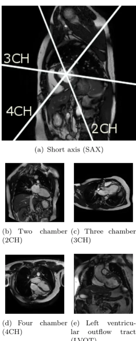
(a) Short axis (SAX)
(b) Two chamber (2CH) (c) Three chamber (3CH) (d) Four chamber (4CH)
(e) Left ventricu-lar outflow tract (LVOT)
Figure 1. Examples and mutual positioning of the short and the main left ventricular long axis cardiac MR views used in this paper. See also Figure 8 which illustrates inter-subject variability of these views.
An excellent introduction to standard MR cardiac ac-quisition planes can be found in Taylor and Bogaert (2012). These planes are often categorised into two groups — the short and the long axis planes. In this paper, we learn to predict the five most commonly used cardiac planes acquired with steady-state free precession (SSFP) acquisition sequences. These are the short axis, 2-, 3- and 4- chamber and left ven-tricular outflow tract views. These five labels are the target of our learning algorithm. See Figure 1 for a visual overview.
The left ventricular short axis slices (Fig-ure 1(a)) are parallel to the mitral valve ring. These are acquired regularly spaced from the cardiac base to the apex of the heart, often as a cine 3D+t stack. These views are excellent for reproducible volumetric measurements or radial cardiac motion analysis, but their use is limited in atrio-ventricular interplay or valvular disease study.
The long axis acquisition planes include the 2-chamber, 3-2-chamber, and 4-chamber views (Fig-ures 1(b) to 1(d)). These planes are used to visualise different regions of the left atrium, mitral valve ap-paratus and the left ventricle. The 3-chamber and left ventricular outflow tract (also known as the coronal oblique view) (fig. 1(e)) views provide visual-isation of the aortic root from two orthogonal planes. The 4-chamber view enables visualisation of the tri-cuspid valve and right atrium.
1.2 Previous work
The previous work on cardiac view recognition has been concentrated mainly on real-time recogni-tion of cardiac planes for echography (Otey, Bi, et al. 2006; Park and Zhou 2007; Park, Zhou, et al. 2007; Beymer and Syeda-Mahmood 2008). There exists some work on magnetic resonance (Zhou, Peng and Zhou 2012; Margeta, Criminisi, et al. 2014; Shaker, Wael, et al. 2014). These methods use dynamic active shape models (Beymer and Syeda-Mahmood 2008), require to train part detectors (Park, Zhou, et al. 2007) or landmark detectors (Zhou, Peng and Zhou 2012). Therefore, any new view will require these extra annotations to be made. Otey, Bi, et al. (2006) avoid this limitation by training an ultrasound cardiac view classifier using gradient-based image features. Margeta, Crim-inisi, et al. (2014) trained classification forests to predict the cardiac planes directly from cardiac MR image miniatures. Shaker, Wael, et al. (2014) recently proposed a technique based on autoen-coders. They learn image representations in an unsupervised fashion and use this representation to distinguish between two cardiac views. We will later show that our proposed method reaches a very favourable performance and surpasses the previously introduced Margeta, Criminisi, et al. (2014). We report the results on an open cardiac data-set which simplifies direct comparison of these different techniques in the future.
The state of the art in image recognition has been heavily influenced by the seminal works of Krizhevsky, Sutskever and Hinton (2012) and Ciresan, Meier and Schmidhuber (2012) using convolutional neural networks (CNNs). Krizhevsky, Sutskever and Hinton (2012) trained a large (60 million parameters) CNN on a massive data-set consisting of 1,2 million images and 1000 classes Russakovsky, Deng, et al. (2014).
They employed two major improvements: Rectified linear unit nonlinearity to improve conver-gence, and Dropout (Hinton, Srivastava, et al. 2012). The Dropout means that during the training phase the output of each hidden neuron is dropped out (set to 0) with a certain probability p. The dropped out neurons do not contribute to the forward pass and are skipped in the back-propagation. For every training, batch a different set of neurons is dropped out i.e. a different network archi-tecture is sampled. At test time, however, all neurons are used and their output responses are multiplied by 1 − p to compensate for the architecture difference. Hinton, Srivastava, et al. (2012) showed that this strategy helps to reduce complex coadaptations of the neurons (as neurons learn not to rely on single neuron responses from the preceding layer) and to reduce overfitting.
Training a large network from scratch without a large number of samples still remains a challeng-ing problem. A trained CNN can be adapted to a new domain by reuschalleng-ing already trained hidden layers of the network, though. It has been shown, for example, by Razavian, Azizpour, et al. (2014) that the classification layer of the neural net can be stripped, and the hidden layers can serve as excellent image descriptors for a variety of computer vision tasks (such as for photography style recognition by (Karayev, Trentacoste, et al. 2013)). Alternatively, the prediction layer model can be replaced by a new one and the network parameters can be fine-tuned through backpropagation. In this paper, we consider all of these approaches (training a network from scratch, reusing a hidden layer features from a network trained on another problem, and fine-tuning of a pretrained network) for using a CNN in cardiac view recognition and compare it with with the prior methods based on random forests using pixel intensities from image miniatures or image plane normal vectors as features.
1.3 Paper structure
In this paper, we compare the three groups of methods for automatic cardiac acquisition plane recognition. The first one is based on DICOM meta-information, and the other two completely ignore the DICOM tags and learn to recognise cardiac views directly from image intensities. In Section 2.1, we first present the recognition method using DICOM-derived features (the image plane orientation vectors). Here, we train a random forest classifier using these three-dimensional feature vectors. We recall (Section 2.2) the previously presented random forest-based method (Mar-geta, Criminisi, et al. 2014). The newly proposed third path using convolutional neural networks is described in Section 2.3. The later two learn to recognise cardiac views from image content without using any DICOM meta information. In Section 3, we compare these approaches. Finally, in Section 4 we present and discuss our results.
1.4 Contributions
The main contribution of our paper is that a good cardiac view recogniser (reaching state of the art performance) can be efficiently trained end-to-end without designing features using a convolutional neural network. This is possible by fine-tuning parameters of a network previously trained for a large-scale image recognition problem.
• We achieve state of the art performance in cardiac view recognition by learning an end-to-end system from raw image intensities using CNNs.
• This is one of the first papers to demonstrate the value of features extracted from medical images using CNNs trained on a large-scale visual object recognition data-set.
good strategy that helps to improve performance and speed up the network training. • We show that the CNNs can be applied to smaller data-sets (a common problem in medical
imaging), thanks to careful network initialisation and data-set augmentation.
2. Methods
A ground truth target label (2CH, 3CH, 4CH, LVOT or SAX) was assigned to each image in our training set by an expert in cardiac imaging. We use it only in the training phase as a target to train and to validate the view recognisers. At the testing phase, we will predict this label from the features. In the paper, we compare two types of methods. The first one is using three-dimensional feature vectors (image plane normal vector) computed from the DICOM orientation tag (Section 2.1) and a random forest classifier which is trained to predict cardiac views using this vector. Algorithms in the second group learn to predict the target labels from the image content (pixel intensities) directly without the need for DICOM tags. This group includes the random forest classifier with image miniatures (Section 2.2) and all convolutional neural network approaches (Section 2.3). Apart from the view label linked to each image in the training set, no other information is necessary to train the classification models. To increase the number of the training samples (for image content-based algorithms), we augment the data-set with small label preserving transformations such as image translations, rotations, and scale changes. See Section 2.2.2 for more details.
2.1 Using DICOM Meta-information: Plane normal + Forest
Figure 2. DICOM plane normals for different cardiac views (Margeta, Cri-minisi, et al. 2014). In our data-set dis-tinct clusters can be observed (best viewed in colour). Nevertheless the separation might not be the case for a more diverse collection of images. Moreover, as we cannot always rely on the presence of this tag, so an image-content-based recogniser is necessary.
Both Zhou, Peng and Zhou (2012) and Margeta, Criminisi, et al. (2014) showed that where the DICOM orientation (0020,0037) tag is present we can use it to predict the cardiac image acqui-sition plane (See Fig.
This method uses feature vectors computed from the DICOM orientation tag and cannot be used in the absence of this tag. This happens, for example, after DICOM tag removal after an incorrectly configured anonymisation procedure, when parsing images from clinical journals or using other image formats. In these cases, we have to rely on recognition methods using exclu-sively the image content. In the next two sections, we present two such methods. One that is based on previous work using de-cision forests and image miniatures (Margeta, Criminisi, et al. 2014) and the other one is a new approach using convolutional neural networks. We learn to predict the cardiac views from 2D image slices individually, rather than using 2D + t, 3D or 3D + t volumes. This decision makes our methods more flexible and ap-plicable also to view recognition scenarios when only 2D images are present, e.g. when parsing clinical journals or images from the web.
2.2 View recognition from image miniatures: Miniatures + forest
This simple method (Margeta, Criminisi, et al. 2014) was posed as a standard image recognition framework where features are extracted from the images and are fed to a classifier (Figure 3), in this case a classification forest. Classification forest (Breiman 1999) is an ensemble learning method that constructs a set of randomised binary decision trees. Its advantage is computational efficiency
Crop central square
Classification forest
Jitter (translate, rotate, scale)
and crop training slices
Miniat ures and intensit y pooling Tra ining Testi ng 2CH 3CH 4CH SAX 2CH 3CH 4CH SAX 2CH 3CH 4CH SAX LVOT LVOT LVOT
Figure 3. Classification forest pipeline for view recognition from image miniatures (Margeta, Criminisi, et al. 2014). Discrimi-native pixels from image miniatures are chosen from a random pool as features for a classification forest. The training data-set is augmented to improve robustness to the differences in the acquisitions without the need for extra data and labels.
and automatic selection of relevant features. At training time, the tree structure is optimised by recursively partitioning the data points into the left or the right branches such that points having the same label are grouped together and points with different labels are put apart. Each node of the tree sees only a random subset of the feature set and greedily picks the single most discriminative feature. This helps to make the trees in the forest different from each other and leads to better generalisation. At test time, features chosen at the training stage are extracted and the images are passed through the trees and reach a set of leaves. Class distributions of all reached leaves are averaged across the forest and the most probable label is selected as the image view. See Criminisi, Shotton and Konukoglu (2011) for a detailed discussion on decision forests.
2.2.1 Using image miniatures
2CH 3CH 4CH LVOT SAX
Figure 4. Averages of the DETERMINE data-set for each cardiac view after cropping the central square. A rea-sonable alignment of cardiac structures can be observed in the data-set. The cardiac cavities and main thoracic structures can be seen.
The radiological images are mostly acquired with the object of interest in the image centre and some rough alignment of structures can be ex-pected (See Figure 4). Image intensity samples at fixed positions (without extra registration) there-fore provide strong cues about the position of dif-ferent tissues (e.g. dark lungs in the top left corner or bright cavity in the centre).
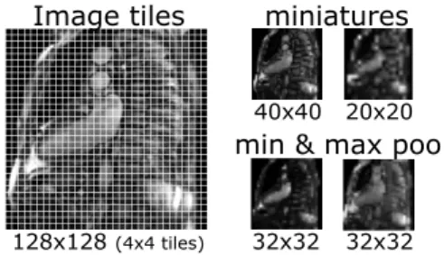
The central square from each image is ex-tracted, resampled to 128x128 pixels and linearly rescaled to range between 0 and 255. We subsam-ple the cropped centers to two fixed sizes (20x20 and 40x40 pixels). In addition, we divide the
im-age into non-overlapping 4x4 tiles and compute intensity minimum and maximum for each of these tiles (Figure 5). This creates a set of pooled image miniatures (32x32 pixels each).
128x128 (4x4 tiles)
40x40 20x20
32x32 32x32
miniatures
min & max pool Image tiles
Figure 5. Image miniatures by min- and max-pooling local intensities (Margeta, Cri-minisi, et al. 2014).
The pooling adds some invariance to small image trans-lations and rotations (whose effect is within the tile size). The pixel values at random positions of these miniature channels are then used directly as features. At each node of the tree, 64 random tile locations across all miniatures are tested and the best threshold on this value is selected to divide the data points into the left or the right partitions until not less than two points are left in each leaf. We train 160 such trees. This method is shown in the evaluation as Miniatures + forest.
2.2.2 Augmenting the data-set with jittering
While the object of interest is in general placed at the image centre, differences between various imaging centers and positioning of the heart on the image exist. The proposed miniature features are not fully invariant to these changes. To account for this, the training set was augmented with extra images created by transforming the originals. These were translations (all shifts in x and y between -10 and 10 pixels for a 5x5 grid), but also scale changes (1 — 1.4 zoom factor with 8 steps while keeping the same image size) and in-plane rotations around the image centre (angles between -10 and 10 degrees with 20 steps). The augmented images were resampled with linear interpolation. Note that the extra expense of data-set augmentation is present mainly at the training time. The test time remained almost unaffected except that now a deeper forest could be learnt. The benefit of data-set augmentation is clear, yielding a solid 12.14% gain in the F1 score (F 1 = 2(precision.recall)/(precision + recall)). Results using this augmented data-set are presented in the evaluation as Augmented miniatures + forest. Compared to the preliminary study in Margeta, Criminisi, et al. (2014), we will test this method on a bigger data-set.
2.3 Convolutional neural networks for view recognition
To improve the performance of the forest-based method, we turn to the state of the art in image recognition — the convolutional neural networks. Their principle is rather simple — the input image is convolved with a bank of filters (conv) whose response are fed through a nonlinear function, e.g. a Rectified Linear Unit (ReLU) f (x) = max(0, x). The responses are locally aggregated with max-pooling. The output of the max-pooling creates a new set of image channels which are then fed through another layer of convolutions and nonlinearities. Finally, the fully connected layers (fc) are stacked and connected to a multiway soft-max in order to predict the target label. The role of the max-pooling is similar to the forest-based method i.e. to aggregate local responses and to allow some invariance of the input to small transformations. The parameters of the network such as weights of the convolutional filters are optimised through backpropagation. Using the stochastic gradient descent, the average batch prediction loss (soft-max) is decreased.
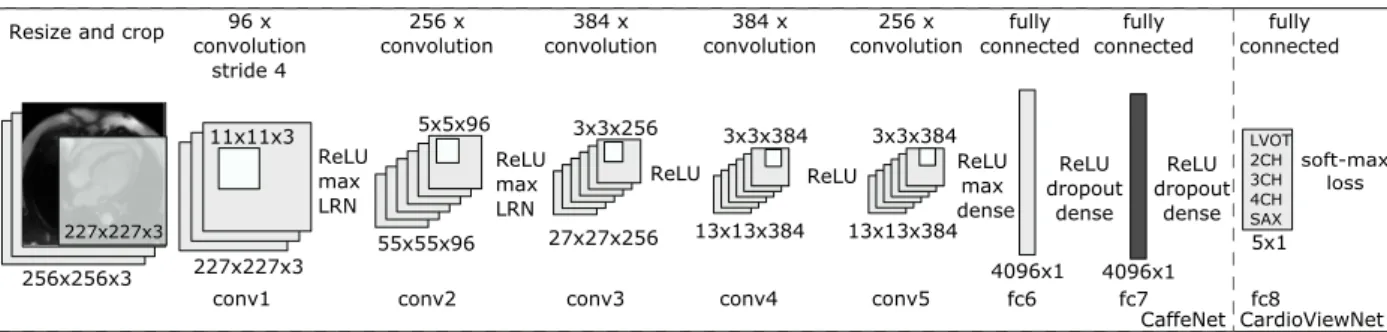
We use the widely adopted neural network architecture (see Figure 6) described by Krizhevsky, Sutskever and Hinton (2012) as implemented in the Caffe framework (Jia, Shelhamer, et al. 2014) under the bvlc reference caffenet acronym (CaffeNet in short). The CaffeNet implementation differs from Krizhevsky’s AlexNet in the order of local response normalisation (LRN) and max-pooling operations. Not only AlexNet/CaffeNet is the winning entry of the ImageNet LSVRC 2012 competi-tion, the weights and definitions of this network are publicly available thus reducing computational time needed for the training and improve reproducibility of this work.
227x227x3 96Ax convolution 11x11x3 256Ax convolution 55x55x96 5x5x96 27x27x256 3x3x256 384AxA convolution 13x13x384 3x3x384 256Ax convolution 4096x1 5x1 fully connected LVOT 2CH 3CH 4CH SAX 256x256x3 ResizeAandAcrop 227x227x3 conv1 conv2 ReLU max LRN conv3 13x13x384 3x3x384 384AxA convolution conv4 conv5 ReLU max LRN
ReLU ReLU ReLUmax
Adense fc6 ReLU dropout dense 4096x1 fc7 ReLU dropout dense fc8 fully connected fully connected soft-max loss CaffeNet CardioViewNet strideA4
Figure 6. Our CardioViewNet is based on CaffeNet network structure and is adapted for cardiac view recognition. We initialised the network weights from a pretrained CaffeNet. We then replaced the last 1000-dimensional logistic regression layer (previous fc8) with a 5-dimensional for 5 cardiac views. Then we fine-tuned the network with our data. We also extracted features from the last 4096-dimensional fully connected layer fc7 (in dark gray) from both CaffeNet and our fine-tuned CardioViewNet and used them with a linear SVM and a decision forest classifier. We achieve the best performance with our fine-tuned network directly. ReLU rectified linear unit, max max pooling, LRN local response normalisation, conv convolutional layer, fc -fully connected layer.
2.3.1 Classifying cardiac views using CNN features optimised for visual recognition
Similarly to the work of Karayev, Trentacoste, et al. (2013) for photography style recognition we use CNN features from a fully connected layer of a network pretrained on the ImageNet LSVRC (Russakovsky, Deng, et al. 2014) data-set. The fully connected layer (in our case fc7 — see Fig-ure 6) helps us to describe the cardiac images with 4096-dimensional featFig-ures. Before putting the cardiac images through the network, simple preprocessing is done. The cardiac images are resized to 256x256 squares regardless of their input dimensions. Since the CaffeNet takes RGB images as input we simply replicate the 2D cardiac slices into each colour channel. We compute a pixel-wise mean image for our cardiac view data-set and subtract it from all training and testing images prior to entering the CNN. This centers image intensities around zero and serves as a very simple intensity normalisation. As we later found in our case, the average image is almost uniform and a scalar value could be subtracted instead. The central (227x227x3) crop of this image is then fed forward through the network. We then use these CaffeNet fc7 features with a linear SVM classi-fier to predict the cardiac views. We ran crossvalidation on the training subset folds to maximise the prediction precision. This helped us to choose the penalty parameter C of the SVM classifier from standard set of values [0.1, 1, 10, 100, 1000] as C = 1. We report results of this method as CaffeNet fc7 + SVM. Similarly, we trained a classification forest (with 64 features tested per node and 1000 trees) using these features (instead of image miniatures) and report these results as CaffeNet fc7 + forest.
These features were adapted to a general object recognition task and come from a CNN that never saw a cardiac MR image to optimise its weights. As we will show in Table 1, this already performs quite well for the cardiac view recognition. In the following we will show how we can further improve performance by adapting the CNN weights to the medical imaging domain. 2.3.2 CardioViewNet architecture and fine-tuning the visual recognition CNN
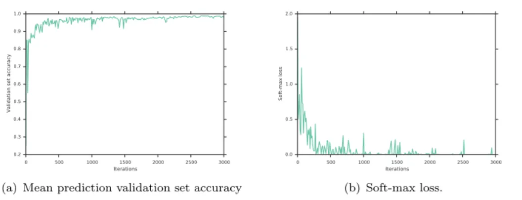
In practise, many examples are often needed to train a large capacity neural network. However, by starting from the weights of a pretrained network, we can just fine-tune the network parameters with new data and adapt it to the new target domain. Here, we use the pretrained CaffeNet (Jia, Shelhamer, et al. 2014) and replace the last 1000-class multinomial regression layer with a 5-class one (See Figure 6). The net is fine-tuned with stochastic gradient descent with higher learning rate (10−2) for parameters in the newly added layer and smaller (10−3) in the rest of the network. We use momentum of 0.9 in the stochastic gradient descent optimiser, and a small weight decay at each iteration (10−4). The batch size used in each iteration was 32 and the step size is kept constant for the whole training. A set of resized 256x256x3 images is used for training. At each iteration, a batch of 32 random (not necessarily central) 227x227x3 crops is extracted from the resized cardiac slices and is fed forward through the network. Compared to the implementation of the forest-based method where all augmented images were precomputed, the translations are cheaply generated on the fly at each iteration. Already after 3000 iterations the prediction error on the validation data-set reaches a plateau and further improvements are only marginal, see Figure 7). We stop the optimisation at 8000 iterations and pick this model in our experiments as it yields the best performance. To reduce overfitting, we use the Dropout strategy (Hinton, Srivastava, et al. 2012) in the fully connected layers fc6 and fc7 with probability of dropping output of a neuron to be 0.5. The fine-tuning is quite efficient and takes approximately 4 hours on a single NVIDIA Tesla M2050 GPU for 8000 iterations. Results of this method are presented as CardioViewNet. We also show results for prediction of an SVM classifier using fc7 features extracted from the fine-tuned network as CardioViewNet fc7 + SVM. In other words, we replace the 1000-class multinomial regression layer of the fine-tuned network by a linear SVM classifier. Results using a classification forest instead are listed as CardioViewNet fc7 + forest. The possibility to replace the final classifier is important for of quick retraining for additional views without extra fine-tuning. In addition to the training set augmentation, we perform oversampling at the test time i.e. average predictions of ten 227x227 image crops: the central crop and the four 227x227 corner aligned
0 500 1000 1500 2000 2500 3000 Iterations 0.2 0.3 0.4 0.5 0.6 0.7 0.8 0.9 1.0
Validation set accuracy
(a) Mean prediction validation set accuracy
0 500 1000 1500 2000 2500 3000 Iterations 0.0 0.5 1.0 1.5 2.0 Soft-max loss (b) Soft-max loss.
Figure 7. Fine-tuning our CardioViewNet model rapidly converges to its best performance.
crops and their horizontally flipped versions (vertically flipped images are rare). We report these results as CardioViewNet + oversample. We will see that this can improve performance on an independent data-set.
2.3.3 Training the network from scratch
Good initialisation of the network is important and the CaffeNet trained on the ImageNet data-set helps us to get well started. The initial motivation behind the fine-tuning was that there were too few images in our data-set to train the whole network from scratch. While the number of images is certainly smaller than in the ImageNet data-set, our target domain is also much simpler. We are predicting only five classes whose appearance variability is lower than the one across the ImageNet classes (e.g. variability of felines in different poses and appearances when they are all labeled as a cat). To test whether there is any value in the fine-tuning instead of learning the network parameters from scratch, we train from the ground up two networks. First, a simpler LeNet-5 network (Lecun, Bottou, et al. 1998) (shown as LeNet-5 from scratch) as defined by Caffe but with the last layer adapted to a 5 class target (similarly to the CardioViewNet). The second network architecture is the CardioViewNet (CardioViewNet from scratch). We found the choice of the learning rate (10−3 for CardioViewNet and 10−5 for LeNet-5, both using batch sizes of 32) and good random initialisation to be crucial to avoid divergence. We initialise the weights with the procedure described by He, Zhang, et al. (2015) that is well suited for networks with the ReLU nonlinearity and choose the learning rate by trial and error, i.e. reducing the learning rate until the network starts to reduce the loss without diverging.
3. Validation
We trained and validated these methods on a data-set of slices from 200 patients (2CH: 235, 3CH: 225, 4CH: 280, LVOT: 12, SAX:2516) from a multi-centre study on post myocardial infarction hearts DETERMINE (Kadish, Bello, et al. (2009)) from steady state free precession (SSFP) acquisition sequence (fig. 8). The LVOT views are severely underrepresented and served us as a test case for learning from very few examples. They are not taken into the account in the mean scores in the results as it would make unrealistic variation between the methods based on chance. We ran a randomised 10-fold cross validation by taking a random subset of 90% of the patients (rather than image slices) for training and used remaining 10% for validation. The patient splits guarantee that repeated acquisitions from the same patient that are occasionally present in the data-set never appear in both the training and the validation set and do not bias our results. Classification accuracy is not a good measure for imbalanced data-sets as performance on the dominant class (i.e. short axis) can obfuscate the true performance. Therefore, in this paper we report means and standard deviations of average (averaging is done across the classes) precisions,
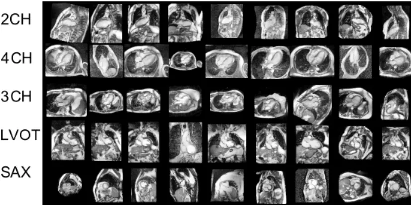
2CH 4CH 3CH LVOT SAX
Figure 8. Typical examples of the training images from the DETERMINE data-set for different views. Note the acquisition and patient differences. In addition, the short axis slices cover the heart from the apex to the base with quite different appearances.
DETERMINE KCL
F1 score precision recall F1 score precision recall DICOM tag based prediction
Plane normal + forest ( 99.14 ± 1.2399.14 ± 1.2399.14 ± 1.23 98.91 ± 1.1398.91 ± 1.1398.91 ± 1.13 99.20 ± 1.5399.20 ± 1.5399.20 ± 1.53 99.08 ± 0.4699.08 ± 0.4699.08 ± 0.46 98.76 ± 0.7898.76 ± 0.7898.76 ± 0.78 99.16 ± 0.3299.16 ± 0.3299.16 ± 0.32 Image content-based prediction
Miniatures + forest ( 59.33 ± 4.15 62.13 ± 5.74 55.61 ± 3.80 39.36 ± 1.75 42.71 ± 4.63 37.98 ± 4.39 Augmented miniatures + forest ( 71.46 ± 2.68 72.33 ± 2.77 68.01 ± 2.65 48.87 ± 2.02 54.74 ± 2.33 43.77 ± 1.98 CaffeNet fc7 + forest ( 75.94 ± 4.50 94.03 ± 1.75 69.08 ± 4.53 88.09 ± 1.29 92.60 ± 1.63 86.86 ± 1.08 CaffeNet fc7 + SVM ( 91.86 ± 4.33 92.48 ± 3.98 91.61 ± 4.71 86.72 ± 1.49 86.70 ± 2.19 87.30 ± 1.08 CardioViewNet fc7 + forest ( 97.48 ± 2.34 98.28 ± 1.84 96.81 ± 3.03 93.43 ± 2.05 95.79 ± 3.10 91.67 ± 2.34 CardioViewNet fc7 + SVM ( 97.39 ± 2.27 98.37 ± 1.8898.37 ± 1.8898.37 ± 1.88 96.65 ± 2.77 88.40 ± 1.84 97.51 ± 2.0297.51 ± 2.0297.51 ± 2.02 88.95 ± 4.44 CardioViewNet ( 97.66 ± 2.0497.66 ± 2.0497.66 ± 2.04 97.82 ± 1.93 97.62 ± 2.3797.62 ± 2.3797.62 ± 2.37 91.01 ± 3.29 92.23 ± 3.80 90.57 ± 3.26 CardioViewNet oversample ( 97.53 ± 2.06 97.98 ± 2.12 97.30 ± 2.30 93.50 ± 3.1293.50 ± 3.1293.50 ± 3.12 95.31 ± 5.17 92.62 ± 2.3092.62 ± 2.3092.62 ± 2.30 LeNet-5 from scratch ( 69.59 ± 5.12 76.79 ± 5.40 67.89 ± 4.26 63.81 ± 4.88 72.03 ± 9.67 60.41 ± 4.53 CardioViewNet from scratch ( 92.36 ± 3.51 92.63 ± 4.44 92.97 ± 2.79 79.72 ± 3.65 80.39 ± 5.39 81.65 ± 3.64
Table 1. Evaluation of the algorithms in the two groups of algorithms, we highlight in bold the best performance from each group. Note: References to relevant sections in the paper with more details on each algorithm are given in the parentheses. We computed average of individual view F1 scores, precisions and recalls for each fold (except for the underrepresented LVOT) for the two data-sets. Here, we display means and standard deviations of these average scores across all 10 folds. The prediction using classification forests on the DICOM orientation vector is the best performing method. However, from purely image-based methods, the fine-tuned convolutional network CardioViewNet outperforms the rest.
recalls and F1 scores. In the context of content-based retrieval, these measures can be interpreted as following: The precision (also known as positive predictive value or false positive rate is defined as TP / (TP + FP )) is the fraction of relevant images (having the same view as the query view) out of all returned images. The recall (also known as sensitivity or true positive rate is defined as TP / (TP + FN ) ) is the probability of retrieving a relevant image out of all existing relevant images, where TP is the number of true positives, FP the number of true negatives, and FN the number of false negatives. The F1 score is the harmonic mean of the precision and the recall.
To study the robustness of the presented algorithms against the data-set bias, we trained recog-niser models from different folds trained exclusively on the DETERMINE data-set (Kadish, Bello, et al. (2009)) and tested them on a completely independent data-set - the STACOM motion tracking challenge (Tobon-Gomez, De Craene, et al. 2013) (KCL in short) containing slices from 15 patients (2CH:15, 4CH:15, SAX:207). The KCL data-set consists of healthy volunteers and the images are in general of higher and more uniform quality and with more consistently chosen regions of interest. This allows us to evaluate performance on the 3 cardiac views present. We invite the interested readers to look at this open access data-set through the Cardiac Atlas Project website (Fonseca, Backhaus, et al. 2011).
4. Results and discussion
Here we present results for the method using DICOM based prediction and methods using image content. The mean average F1 scores, precisions and recalls are summarised in Table 1 and total confusion matrices for the two best methods from each family (DICOM based and Image-based) can be seen in Figure 9. We confirm findings from the previous work that cardiac views can be predicted from image plane normals and serve as a prior (Zhou, Peng and Zhou 2012) but require presence of the relevant DICOM tag. The larger DETERMINE data-set turned out to be more challenging for the miniature-based method and it performed significantly worse than in the results published previously. On the contrary, the performance of the CaffeNet features for cardiac view description is quite remarkable. These were not trained for cardiac MR images yet they perform better than most methods with handcrafted features. They most likely encode local texture statistics which helps with the prediction. Adding some texture channels to the miniature method could therefore improve the performance.
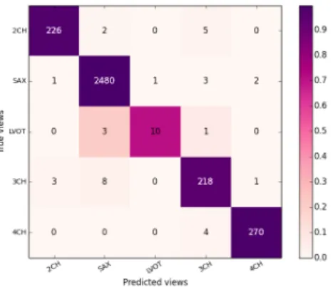
(a) Predictions from DICOM-derived image normals (Plane normal + forest).
(b) Predictions from image content with a fine-tuned CNN (CardioViewNet).
Figure 9. Sum of the confusion matrices over the 10 folds of our crossvalidation on the DETERMINE data-set for the best model classifying images using DICOM normal information and the best image-based predictor (using our fine-tuned neural network).
The quality of predictions using the fine-tuned CardioViewNet is almost on par with the ap-proach using DICOM-derived information and significantly outperforms the previous forest-based method using image miniatures (Margeta, Criminisi, et al. 2014) while not requiring to train any extra landmark detectors as in Zhou, Peng and Zhou (2012). As features extracted from the Car-dioViewNet do a good job even when used with external classifiers, they could be used to learn
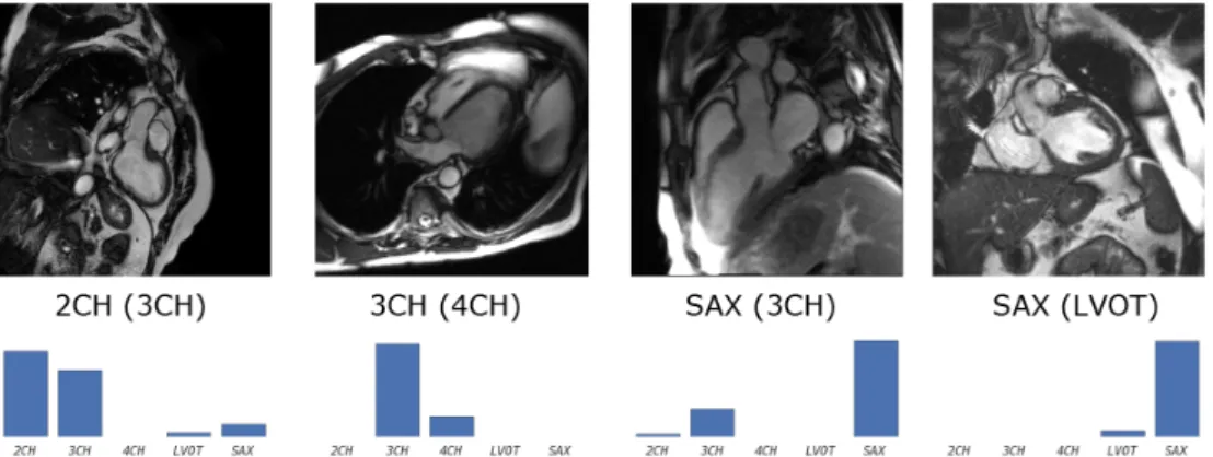
Figure 10. Examples for some of the least confident correct (the normal predictions are usually very peaky) predictions using CardioViewNet. Predicted and true (in parentheses) labels shown under the images. Below them are view-specific prediction confidences.
Figure 11. Example misclassifications using CardioViewNet. Predicted and true label (in parentheses) are indicated under the images and below them are view-specific prediction confidences. The failures typically happen with less typical acquisitions and truly ambiguous images. The misclassified 2CH image indeed looks like a 3CH image except that the left atrium is missing and the ventricle is acquired at a non standard oblique angle. Similarly for the 4CH view, the right atrium is missing and one can already see parts of the outflow tract branching out of the left ventricle typical for a 3CH view. The 3CH view is captured with a detailed region of interest not very common in the data-set. Extra data augmentation could probably help to fix this case. Finally, the LVOT views are severely under-represented and can be confused with basal short axis views. Note that for all of these cases, the correct prediction is in the top two most likely views.
extra view recognisers without additional fine-tuning on these. In Figure 10 we present examples of some of the least confident correct predictions using the fine-tuned CardioViewNet. It is important to note that the softmax output of the neural network not only returns the label but also some measure of confidence in the prediction. Similarly, the incorrectly classified images (see Figure 11) often belong to views more difficult to recognise for a human observer and the second best predic-tion is the correct result. When training from scratch, the performance does not seem to improve beyond 10,000 iterations and we pause the backpropagation there. Although the performance is much lower than for the fine-tuned networks, the network learns to predict the cardiac views. For the LeNet-5 model trained from scratch, the performance closely follows the CaffeNet fc7 + SVM model. We did not observe any benefit of using forests (at least when using orthogonal splits) over the linear SVM when using features from the convolutional nets and the forest performs in general worse. The performance of the CardioViewNet trained from scratch is better than using the fully connected layer features (fc7 ) from CaffeNet but the training takes significantly longer to obtain. The predictions on the KCL data-set are naturally slightly worse as some differences between the studies still exist. We have observed that test time oversampling (averaging predictions of the central and corner patches and their horizontally flipped versions) improves the scores for this data-set although it does not improve the DETERMINE data-set predictions. This might indicate that a better thought oversampling, image normalization or data-set augmentation strategies might further improve the cross-data-set generalisation.
5. Conclusion
Convolutional neural networks and features extracted from them seem to work remarkably well for medical images. As large data-sets to train complex models are often not available, retargeting the domain of a previously trained model by fine-tuning can help. This speeds up the learning process and achieves better predictions. Even models trained for general object recognition might be a great baseline to start. In our case, doing network surgery and fine-tuning the pretrained model allowed us to make significant progress in cardiac view recognition from image content without handcrafting the features or training with extra annotations. This also allowed us to gain performance over models learnt from scratch. However, even the performance of models learnt from scratch is very encouraging for further exploration. Features extracted from our network should be useful as descriptors for new views and extend our method even to other pathology specific views
(such as those used in congenital heart diseases) and acquisition sequences other than SSFP, and even to recognise the acquisition sequences themselves. The methods presented in this paper are important additions to the arsenal of tools for handling noisy metadata in our data-sets and are already helping us to organise collections of cardiac images. In the future this method will be used for semantic image retrieval and parsing of medical literature.
Conflict of interest disclosure statement
No potential conflict of interest was reported by the authors.
Acknowledgments
We used data and infrastructure made available through the Cardiac Atlas Project (www.cardiacatlas.org - Fonseca, Backhaus, et al. (2011)). See Kadish, Bello, et al. (2009), Tobon-Gomez, De Craene, et al. (2013) for more details on the data-sets. DETERMINE was supported by St Jude Medical, Inc; and the National Heart, Lung and Blood Institute (R01HL91069). A list of participating DETERMINE investigators can be found at http://www.clinicaltrials.gov. This work uses scikit-learn toolkit (Pedregosa, Varoquaux, et al. (2011)) for decision forests and Caffe deep learning framework (Jia, Shelhamer, et al. (2014)) for training of the convolutional neural network and the pretrained model (CaffeNet). This model was trained on a subset (Russakovsky, Deng, et al. 2014) of the ImageNet (Deng, Dong, et al. 2009) data-set.
Funding
This work was supported by Microsoft Research through its PhD Scholarship Programme and ERC Advanced Grant MedYMA 2011-291080. The research leading to these results has received funding from the European Unions Seventh Framework Programme for research, technological development and demonstration under grant agreement no. 611823 (VP2HF).
References
Beymer D, Syeda-Mahmood T. 2008. Exploiting spatio-temporal information for view recognition in cardiac echo videos. 2008 IEEE Computer Society Conference on Computer Vision and Pattern Recognition Workshops:1–8.
Breiman L. 1999. Random forests-random features:1–29.
Ciresan D, Meier U, Schmidhuber J. 2012. Multi-column deep neural networks for image classification. In: Computer Vision and Pattern Recognition (CVPR), 2012 IEEE Conference on; June. p. 3642–3649. Criminisi A, Shotton J, Konukoglu E. 2011. Decision Forests: A Unified Framework for Classification,
Re-gression, Density Estimation, Manifold Learning and Semi-Supervised Learning. Foundations and Trends in Computer Graphics and Vision. 7(2-3):81–227.
Deng J, Dong W, Socher R, jia Li L, Li K, Fei-fei L. 2009. Imagenet: A large-scale hierarchical image database. In: In CVPR.
Fonseca C, Backhaus M, Bluemke D, Britten R, Chung J, Cowan B, Dinov I, Finn J, Hunter P, Kadish A, et al. 2011. The Cardiac Atlas Project- an Imaging Database for Computational Modeling and Statistical Atlases of the Heart. Bioinformatics. 27(16):2288–2295.
He K, Zhang X, Ren S, Sun J. 2015. Delving Deep into Rectifiers: Surpassing Human-Level Performance on ImageNet Classification. ArXiv e-prints.
Hinton GE, Srivastava N, Krizhevsky A, Sutskever I, Salakhutdinov RR. 2012. Improving neural networks by preventing co-adaptation of feature detectors:1–18. Available from: http://arxiv.org/abs/1207.0580.
Jia Y, Shelhamer E, Donahue J, Karayev S, Long J, Girshick R, Guadarrama S, Darrell T. 2014. Caffe: Convolutional Architecture for Fast Feature Embedding. arXiv preprint arXiv:14085093.
Kadish AH, Bello D, Finn JP, Bonow RO, Schaechter A, Subacius H, Albert C, Daubert JP, Fonseca CG, Goldberger JJ. 2009. Rationale and design for the Defibrillators to Reduce Risk by Magnetic Resonance Imaging Evaluation (DETERMINE) trial. Journal of cardiovascular electrophysiology. 20(9):982–7. Karayev S, Trentacoste M, Han H, Agarwala A, Darrell T, Hertzmann A, Winnemoeller H. 2013. Recognizing
Image Style:1–20. Available from: http://arxiv.org/abs/1311.3715.
Krizhevsky A, Sutskever I, Hinton G. 2012. ImageNet Classification with Deep Convolutional Neural Net-works. In: Advances in Neural Information Processing Systems.
Lecun Y, Bottou L, Bengio Y, Haffner P. 1998. Gradient-based learning applied to document recognition. Proceedings of the IEEE. 86(11):2278–2324.
Margeta J, Criminisi A, Lee DC, Ayache N. 2014. Recognizing cardiac magnetic resonance acquisition planes. In: Medical Image Understanding and Analysis. London, United Kingdom: Reyes-Aldasoro, Constantino Carlos and Slabaugh, Gregory. Available from: https://hal.inria.fr/hal-01009952.
Otey M, Bi J, Krishna S, Rao B. 2006. Automatic view recognition for cardiac ultrasound images. In: International Workshop on Computer Vision for Intravascular and Intracardiac Imaging. p. 187–194. Park J, Zhou S. 2007. Automatic cardiac view classification of echocardiogram. ICCV 2007.
Park JH, Zhou SK, Simopoulos C, Otsuki J, Comaniciu D. 2007. Automatic Cardiac View Classification of Echocardiogram. IEEE 11th International Conference on Computer Vision:1–8.
Pedregosa F, Varoquaux G, Gramfort A, Michel V, Thirion B, Grisel O, Blondel M, Prettenhofer P, Weiss R, Dubourg V, et al. 2011. Scikit-learn: Machine Learning in Python. Journal of Machine Learning Research. 12:2825–2830.
Razavian AS, Azizpour H, Sullivan J, Carlsson S. 2014. CNN Features off-the-shelf: an Astounding Baseline for Recognition. Available from: http://arxiv.org/abs/1403.6382.
Russakovsky O, Deng J, Su H, Krause J, Satheesh S, Ma S, Huang Z, Karpathy A, Khosla A, Bernstein M, et al. 2014. ImageNet Large Scale Visual Recognition Challenge:37.
Shaker M, Wael M, Yassine I, Fahmy A. 2014. Cardiac mri view classification using autoencoder. In: Biomed-ical Engineering Conference (CIBEC), 2014 Cairo International; Dec. p. 125–128.
Taylor AM, Bogaert J. 2012. Cardiovascular MR Imaging Planes and Segmentation. In: Bogaert J, Dy-markowski S, Taylor AM, Muthurangu V, editors. Clinical cardiac mri se - 333. Springer Berlin Heidelberg; p. 93–107. Medical Radiology; Available from: http://dx.doi.org/10.1007/174_2011_333.
Tobon-Gomez C, De Craene M, McLeod K, Tautz L, Shi W, Hennemuth A, Prakosa A, Wang H, Carr-White G, Kapetanakis S, et al. 2013. Benchmarking framework for myocardial tracking and deformation algorithms: An open access database. Medical image analysis. 17(6):632–48.
Zhou Y, Peng Z, Zhou X. 2012. Automatic view classification for cardiac MRI. In: 9th IEEE International Symposium on Biomedical Imaging (ISBI). Barcelona: IEEE; p. 1771–1774.