Computational 3D and reflectivity imaging with high photon efficiency

(1)

Computational 3D and Reflectivity Imaging

with High Photon Efficiency

by

Dongeek Shin

Submitted to the Department of Electrical Engineering and Computer

Science

_RH

3 in partial fulfillment of the requirements for the degree of

MASSACHUSETS WT

OF TECHNOLOGY

Master of Science in Computer Science and Engineering

₉

_{JUN 10 2014}

at the

LIBRARIES

MASSACHUSETTS INSTITUTE OF TECHNOLOGY

June 2014

©

Massachusetts Institute of Technology 2014. All rights reserved.

Signature redacted

A uthor ...

...

Department of Electrical Engjneering and Computer Science

Certified by...

SI

Certified by. .

Signature redacted

"1I

May

21,

Z04

...

Vivek K Goyal

Assistant Professor, Boston University

ignature redacted

Thesis Supervisor

Jeffrey H. Shapiro

Julius A. Stratton Professor

Thesis Supervisor

Accepted by ...

Signature redacted

/

07 J

Leslie Kolodziejski

Chairman, Department Committee on Graduate Theses

(2)

(3)

Computational 3D and Reflectivity Imaging

with High Photon Efficiency

by

Dongeek Shin

Submitted to the Department of Electrical Engineering and Computer Science on May 21, 2014, in partial fulfillment of the

requirements for the degree of

Master of Science in Computer Science and Engineering

Abstract

Imaging the 3D structure and reflectivity of a scene can be done using photon-counting detectors. Traditional imagers of this type typically require hundreds of detected photons per pixel for accurate 3D and reflectivity imaging. Under low light-level conditions, in which the mean photon count is small, the inverse problem of forming

3D and reflectivity images is difficult due to the Poisson noise inherent in low-flux

operation. In this thesis, we propose and study two computational imagers (one passive, one active) that can form accurate images at low light levels. We demonstrate the superior imaging quality of the proposed imagers by comparing them with the state-of-the-art optical imaging techniques.

Thesis Supervisor: Vivek K Goyal

Title: Assistant Professor, Boston University

Thesis Supervisor: Jeffrey H. Shapiro Title: Julius A. Stratton Professor

(4)

(5)

Acknowledgments

I am very fortunate to have Professor Vivek Goyal and Professor Jeffrey Shapiro as my research supervisors. I thank Vivek for being supportive ever since I joined the STIR group and guiding me and my research during my first two years at MIT.

I would like to thank Jeff for his great mentorship and teaching me how to be a

meticulous researcher. Every research meeting with Vivek and Jeff has enlightened me and affected this thesis in positive ways.

I would like to thank Ahmed Kirmani, who motivated me further to look into the topic of time-resolved imaging and gave me invaluable advice on many ideas that went into this thesis.

I would also like to thank my research collaborators Andrea Colago, Dheera Venka-traman, Dr. Franco Wong, and Hye Soo Yang for creating the synergy that improved the quality of my research as a whole.

Finally, I thank my family for their endless love and support.

This research was supported in part by NSF grant No. 1161413 and a Samsung Scholarship.

(6)

(7)

. . . .

50

. . . . 50 . . . . 51 . . . . 52 . . . . 53 . . . . 56 . . . . 56 . . . . 58 . . . . 58 63 63 63 65 65 66 68 69 70 71 73 74 75

(9)

List of Figures

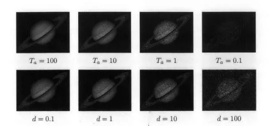
2-1 Effect of shot noise on image quality for several acquisition times Ta (top) and dark count rate values d (bottom). The maximum reflectivity value of the saturn image is 25. . . . . 19

2-2 The multiplexed imaging setup. Measurement zi is collected using pattern wi for i = 1, 2,... n, where n is the total number of image

p ix els. . . . . 21

2-3 The non-negative orthant cone and the polyhedral cone c(W), assum-ing zero dark count. True reflectivity image (black) lies in the non-negative orthant. From one realization of data, we obtain a feasible reflectivity estimate (blue) using the matrix inverse solution. From an-other realization of data, the estimate (red) has negative entries and thus is not valid. . . . . 26

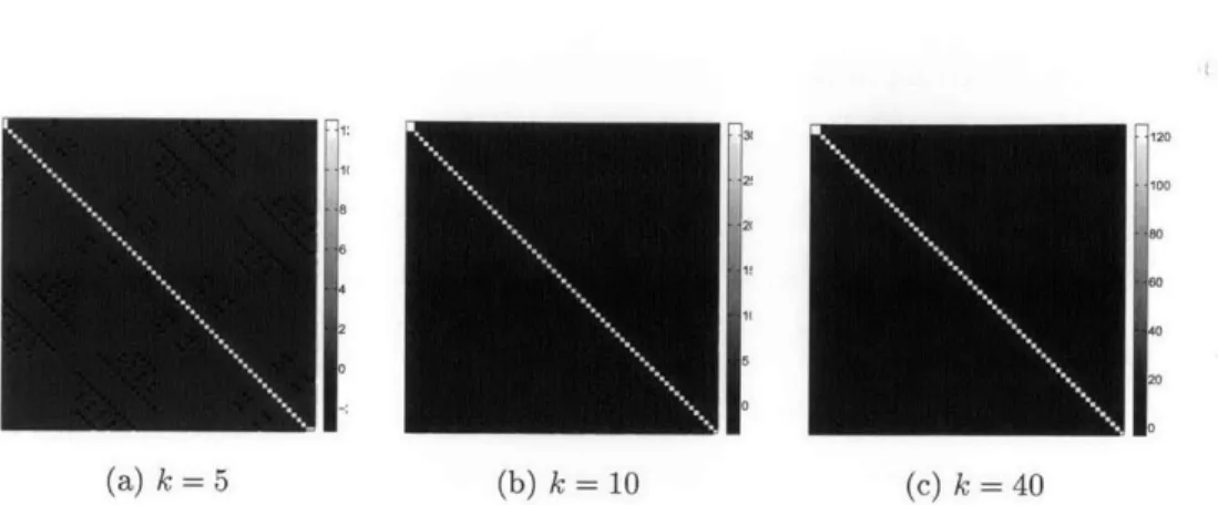
2-4 Covariance matrices of Hadamard inverse solution Rin" for several

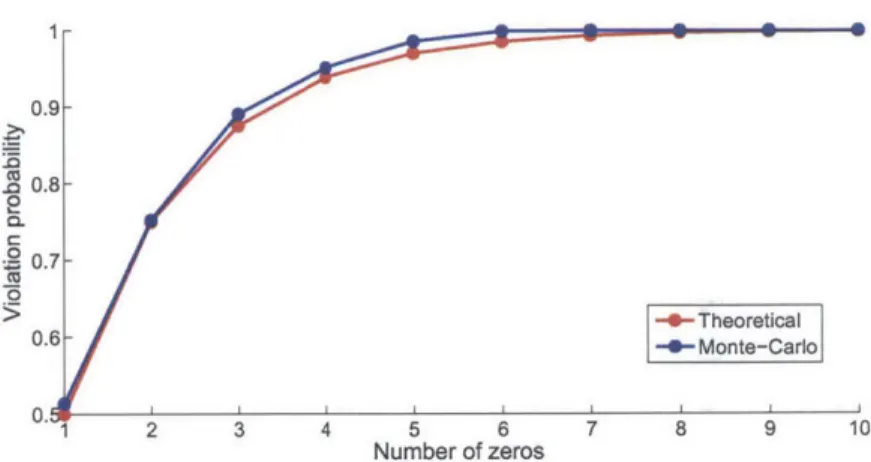
spar-sity levels of size 63 vector x (k is the number of non-zero entries). The non-zero support of x was randomly selected and non-zero entries were set to 100. . . . . 30 2-5 Simulated violation probability using Hadamard multiplexing (blue)

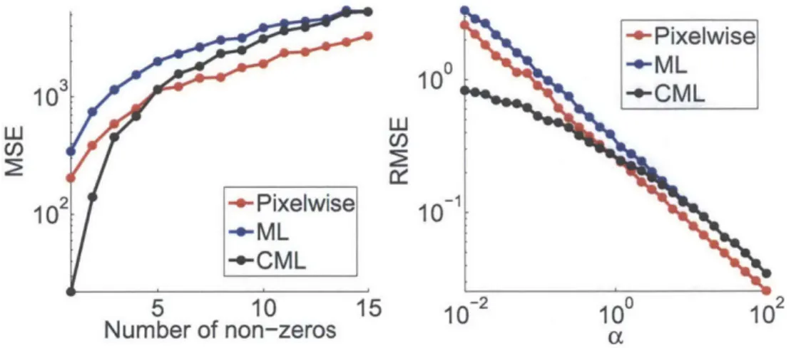
and the derived theoretical lower bound (red) in Equation (2.16) vs. number of zeros. The reflectivity vector x has size 15. The non-zero support of signal x was randomly generated and its non-zero entries w ere all set to 100. . . . . 31 2-6 (Left) MSE vs. number of non-zeros no. (Right) RMSE vs. signal

(10)

2-7 _{Reflectivity estimates of the MIT logo image (top) and the}

Shepp-Logan image (bottom) from traditional pixelwise ML and the proposed CML that uses multiplexed measurements. All images are sized 127 x

129. ... ... ₃₆

2-8 _{Reflectivity estimates of the Mandrill image (top) and the cameraman}

image (bottom) using CPML. All images are sized 127 x 129. .... 37

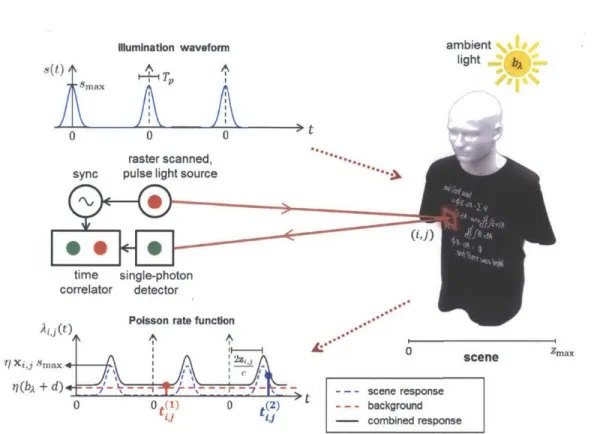
3-1 _{Data acquisition model. Rate function Aj,(t) of inhomogeneous}

Pois-son process combining desired scene response and noise sources is shown for pixel (i, j). Here, N = 3 and kij = 2. A noise photon (red) was detected after the second transmitted pulse at td1), and a signal photon (blue) was detected after the third transmitted pulse at

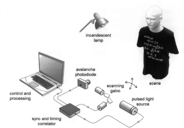
3-2 _{Experimental setup for single-photon imaging. . . . .} ₅₁ 3-3 _{Resolution test experiments. Reflectivity chart imaging (top) was done}

using Ta = 300 ps and mean photon count of 0.48. Depth chart imaging (bottom) was done using Ta = 6.2 ps, mean photon count of 1.1, and 33 % of the pixels missing data. The mean photon count was computed

simply by averaging the number of photon counts at every pixel over the fixed acquisition time. . . . . 52

3-4 Experimental results for imaging natural scenes. . . . . 54

3-5 _{Comparison between our framework and LIDAR technology for 3D}

im aging. _{. . . .} ₅₅

3-6 _{Sample MSE images with 100 independent trials for two natural scenes.} ₅₆ 3-7 Effect of dwell time T and signal-to-background ratio (SBR) on our

3D recovery method. For acquisition times of 100 /Ls and 50 pus, we calculated the mean photon count kij over all pixels to be 1.4 and 0.6, respectively. _{. . . .} ₅₇

3-8 _{Distributions of generalized Gaussian random variables for several}

(11)

3-9 Comparison of MSE of time-delay recovery using single-photon de-tections for two different illumination pulses. (Left) Plot of s,(t), a Gaussian pulse, and s,(t), an arbitrary bimodal pulse. (Right) MSE of ML estimators vs. number of photon detections. . . . . 62

(12)

(13)

Chapter 1 Introduction

Modern optical imaging systems collect a large number of photon detections in order to suppress optical detector noise and form accurate images of object properties. For example, a commercially available digital camera provides the user with a clean pho-tograph by detecting trillions of photons with the sensor array. Traditional imagers are thus required to operate with long acquisition times or at high light levels such that the total optical flux hitting the detector is sufficiently high.

In this thesis, we propose two computational imagers (one passive, one active) that can accurately recover images of scene properties, such as reflectivity and 3D structure, at low-flux regimes where the mean photon count per pixel can even be less than one. The core principle that allows high-quality imaging for both proposed im-agers is the combination of the photodetection physics with the statistical properties of image representations. The proposed imagers are as follows.

1. A single-pixel camera with high photon efficiency: We propose a passive

single-pixel reflectivity imager that can accurately estimate the scene reflectiv-ity in photon-limited imaging scenarios by using an extension of the theory of multiplexed sensing. The proposed method, which makes use of the physically realistic constraint that reflectivity values are non-negative, disproves the ac-cepted wisdom that reflectivity estimation based on multiplexed measurements always degrades imaging performance under low light-level Poisson noise of the

(14)

photodetector. We demonstrate through numerical experiments that the pro-posed imager outperforms the classical single-pixel camera that takes direct raster observations at low light levels.

2. An active 3D imaging system with high photon efficiency: We

pro-pose an active imager that will simultaneously recover scene reflectivity and

3D structure with high accuracy using a single-photon detector. The proposed

imager allows high-quality 3D imaging by combining the accurate single-photon counting statistics with the prior information that natural scenes are spatially correlated. Experimental results show that the proposed imager outperforms state-of-the-art 3D imaging methods that incorporate denoising algorithms. We form accurate 3D and reflectivity images even when the mean number of pho-ton detections at a pixel is close to 1. Also, we give an information-theoretic framework that can be used to choose optimal design parameters such as the illumination pulse shape, at least for the pixelwise imaging scenario.

Higher photon efficiency of an imaging system directly translates to shorter data ac-quisition time. For 3D imaging specifically, it can translate to lower illumination power and longer range imaging. Thus, the theory of highly photon-efficient imag-ing in this thesis opens up many interestimag-ing research areas for buildimag-ing real-time imaging systems that can robustly operate at low-power and under low light-level conditions.

The remainder of the thesis is organized as follows. In Chapter 2, we discuss the single-pixel camera and propose a computational imaging method that achieves high photon efficiency in estimating scene reflectivity. Chapter 3 describes the method of 3D imaging using an active illumination source and a single-photon detector, and proposes a highly photon-efficient computational 3D imaging method. Chapter 4

(15)

Bibliographical Note

Parts of Chapter 2 appear in the paper:

* D. Shin, A. Kirmani, and V. K. Goyal, "Low-rate Poisson intensity estimation using multiplexed imaging", Proceedings of IEEE International Conference on Acoustics, Speech and Signal Processing, 2013, pp. 1364-1368.

Parts of Chapter 3 appear in the papers:

" D. Shin, A. Kirmani, V. K. Goyal, and J. H. Shapiro, "Computational 3D and

reflectivity imaging with high photon efficiency", Accepted for publication at

IEEE International Conference on Image Processing, 2014.

" D. Shin, A. Kirmani, A. Colago, and V. K. Goyal, "Parametric Poisson process

imaging", Proceedings of IEEE Global Conference on Signal and Information Processing, 2013, pp. 1053-1056.

" D. Shin, A. Kirmani, V. K. Goyal, and J. H. Shapiro, "Information in a photon:

relating entropy and maximum-likelihood range estimation using single-photon counting detectors", Proceedings of IEEE International Conference on Image

Processing, 2013, pp. 83-87.

" A. Kirmani, D. Venkatraman, D. Shin, A. Colago, F. N. C. Wong, J. H. Shapiro, and V. K. Goyal, "First-photon imaging", Science, vol. 343, no. 6166, pp. 58-61, 2014.

" A. Kirmani, A. Colago, D. Shin, and V. K. Goyal, "Spatio-temporal

regular-ization for range imaging with high photon efficiency", Proceeedings of SPIE, 2013, vol. 8858, pp. 88581F.

(16)

(17)

Chapter 2 Single-Pixel Reflectivity Imaging with

High Photon Efficiency

2.1 Prior Work

Passive optical imaging relies on an ambient light source to form an image of the scene reflectivity. Commercially available digital cameras are well-known examples of passive optical imagers. Since a two-dimensional sensor array is used for a camera, the reflectivity image is formed by measuring the total optical power hitting the photodetector over a finite acquisition time at every image pixel. The array allows the pixelwise measurements to be made in parallel.

Unlike cameras with a two-dimensional sensor array, the single-pixel camera [1] uses a single photodetector that takes pixelwise measurements not in parallel, but sequentially using a light modulator. The single-pixel camera has its advantages in size, complexity, and cost compared to an array-based camera. However, array based sensing is still preferred over single-pixel sensing when having a short acquisition time is important such as in real-time imaging.

The single-pixel camera is particularly useful in low light-level imaging scenarios, in which one is required to use single-photon avalanche detectors and photomultipliers, that are typically not available as arrays. Accurate formation of intensity images at low light levels is important in engineering applications such as astronomy [21,

(18)

night vision [3], medical imaging applications such as positron emission tomography (PET), and imaging of light-sensitive biological and chemical samples [4]. In all of these applications, the low-light measurements are collected using single-photon detectors. The main challenge is that the measurements made using such detectors are inherently noisy due to low photon-count levels and are thus corrupted by signal-dependent photon noise that comes from the quantum nature of light detection. In this section, we survey several techniques for low light-level imaging using a single-pixel camera equipped with a photon-number resolving detector.

2.1.1 Classical Passive Reflectivity Imaging

Let x be the ideal pixelated scene reflectivity of size n x 1 that we are interested in imaging. If the scene is two-dimensional, then x is its vectorized version. Here, we include the effects of passive illumination and radial fall-off of optical flux in the reflectivity vector x. At every image pixel, we use the photon-counting photodetector to record the number of photons detected in an acquisition time of T. Since we have a total of n image pixels in the single-pixel camera, the total image acquisition time using raster scanning then equals nT.

Let y be the photon count measurement that the photodetector makes at the i-th pixel. In the absence of illumination, our observations y, are simply detector dark counts. We denote the dark count rate as d > 0. We assume that we know d exactly through a calibration process prior to the imaging experiment. The photon counting noise that corrupts our observations is known as shot noise and is well-modeled as Poisson distributed [5]. Our observation model at pixel i is then

yj ~ Poisson(T (xi + d)). (2.1)

The probability mass function of our observation at pixel i is thus

exp{-Ta(xi + d)} (Ta(xi + d))Y(

(19)

Ta = 100 Ta = 10T

d = 0.1 d = 1 d = 10 d = 100

Figure 2-1: Effect of shot noise on image quality for several acquisition times Ta (top) and dark count rate values d (bottom). The maximum reflectivity value of the saturn image is 25.

for yi = 0,1, 2,.... Thus, the maximum-likelihood (ML) pixelwise reflectivity

esti-mate from our data y = [yi,. ., y.]T is simply R = y/Ta - d, where d = [d,.. ., d]T.

We observe that the ML estimate is obtained by normalizing and bias-correcting the raw photon count observations y. The variance of the pixelwise reflectivity estimate R at the i-th pixel is Var(Ri) = (xi + d)/Ta. As shown in Figure 2-1, we observe that

traditional pixelwise ML estimate using the single-pixel camera is limited to having a long acquisition time Ta and low dark count rate d to minimize the variance from shot noise and form high-quality images in photon-limited scenarios.

2.1.2 Single-Pixel Camera based on Compressive Sensing

Recently, the authors of [6] developed an architecture for a photon-efficient single-pixel camera that uses compressed sensing theory. The theory of compressed sensing

171

accurate image formation is guaranteed with high probability even when the num-ber of measurements is less than the numnum-ber of image pixels. Although it uses only one photodetector like the raster-scanned system considered above, the compressed sensing imaging setup has a major difference from that of traditional pixelwise imag-ing. Unlike traditional imaging which involves sensing one image pixel at a time and acquiring n measurements in total, compressive imaging acquires a sequence of m measurements by observing, light from multiple pixels at the same time using

(20)

designed coded patterns. Typically, the structured pattern of pixels can be achieved using a digital micromirror device (DMD). Experimental results in [8] show the high-quality reflectivity images which are formed using traditional scanning method can be obtained using compressed sensing with one tenth the number of total measurements, and thus with higher photon efficiency.

Let {w1, ... , Wm} be the set of m vectors, each of size n x 1, describing the coded pattern of pixelwise measurements. By the optical flux conservation law, we see that every entry of wi must be between 0 and 1, for i = 1, 2,. . ., m. Then, the observation model for the i-th measurement taken by the compressive single-pixel camera is

zi ~ Poisson

(Ta(wTx

+ d)) , (2.3)

where wT _{is the vector transpose of wi. We can also write the observation model in}

matrix-vector form:

z ~ Poisson (Ta(Wx + d)), (2.4)

where now W is an m x n matrix that row-concatenates the n measurement patterns

{wf,...

, w'} and z is the measurement vector of size m x 1. Then, the theory of

robust compressed sensing [91 allows us to have m < n and form accurate reflectivity images with high probability, given that the matrix W satisfies the restricted isometry property (RIP) and the prior information that the image is sparse in the transform-domain.

However, the authors of [10] proved that image estimation based on compressed sensing under low light conditions (Ta(Wx + d)i < 1 for all i E {1,.. . , m}) fails due to the signal-dependent nature of Poisson noise. Thus, at low light levels, it is instead preferable to rely on traditional pixelwise methods described in the previous section than compressive methods. In other words, although compressive single-pixel imaging achieves higher photon efficiency by making fewer total measurements at high light levels, the method has no performance guarantees when the total flux hitting the detector is low and when the effect of shot noise is significant.

(21)

passive source

e 0

Wi

-

1detector object DMD + optics

Figure 2-2: The multiplexed imaging setup. Measurement zi is collected using pattern wi for i = 1, 2, ... n, where n is the total number of image pixels.

2.1.3 Single-Pixel Camera based on Multiplexed Sensing

Multiplexed imaging is another powerful mechanism used to boost imaging perfor-mance when the observation noise is signal independent. Unlike compressed imaging, multiplexed imaging requires the number of measurements of coded patterns to be equal to the number of image pixels (m = n). The multiplexed imaging setup is shown in Figure 2-2. Unlike compressed imaging, the method of multiplexed imag-ing does not require any sparsity assumptions on the scene reflectivity and is thus a non-Bayesian imaging method.

It has been shown [6] that multiplexed imaging outperforms classical pixelwise imaging when the observations are corrupted by signal-independent noise. We em-phasize that this is the case when we are operating with a simple photodiode detector at high light levels, where the effect of shot noise and dark current contribution is minimal. Our measurement vector z of size n can be assumed to be corrupted by additive Gaussian noise:

Z = TaWx +,q, (2.5)

where W

c

[0, 1]"'7 is a square multiplexing matrix and 7 is a vector whose entries are independent and identically distributed (i.i.d.) zero-mean Gaussian random variables with variance ca. Note that if W is the identity matrix, then we have the observation

(22)

model of traditional pixelwise imaging. Assuming that the multiplexing matrix W is non-identity and non-singular, we can decode the multiplexed measurements and estimate the reflectivity image by performing a simple matrix inversion. The matrix inversion estimate -inv = W - 1_{(Z/Ta) is the traditional demultiplexing solution [11J.}

Researchers were interested in using multiplexed measurements instead of direct measurements, with the aim of reducing the mean-square error (MSE). For an es-timator R of x, the MSE is defined as MSE(x, R) = tr (E[(x -- )(x - )T])

,

where tr(-) and E respectively denote the trace and expectation operators. The multiplexing gain 9(W) associated with the multiplexing code W is defined as the reduction ratio in the root MSE from pixelwise imaging to multiplexed imaging:

MSE(x, y/Ta)

9 (W) MSE(x, kinv) (2.6)

We see that 9(W) > 1 implies that multiplexed imaging using pattern W outperforms traditional imaging when the noise is additive Gaussian. In this case, we can write

_(W)

=/tr (E[(x - y/Ta)(x - y/Ta)T]) 9(W) - tr (E[(x - Rinv)(X -- Rifv)T])

_ tr( E [ yT tr(E[W-lrrTWT])

t r(diag( .2 ,' .2])) t~r(W 1d ia g ([0.2, . a2 .])W-T)

tr (WTW)1)'(2.7)

where diag(v) is a matrix that has v as its diagonal and zeros as its off-diagonal entries. Then, the optimal multiplexing pattern that maximizes the gain is obtained

(23)

by solving the following optimization problem: n max (2.8) w tr((WTW)-1) s.t. W i~j E [0, 1], i, I ,.. n IWI -f 0,

where JWI is the determinant of W. The optimization problem in (2.8) is non-convex in W and thus is a difficult problem to solve. However, with the extra constraints that Wjj

E

{0, 1} and that every measurement should combine optical flux from

exactly C pixels, previous works [12] proved that Hadamard multiplexing is optimal for certain values of n. The Hadamard multiplexing matrix H of size n x n can be constructed by deleting the first row and column of a Hadamard matrix of size n + 1 and replacing l's with O's and -I's with l's [111. By construction, the Hadamard multiplexing matrix will have C = (n

+

1)/2 ones and (n - 1)/2 zeros at every row. Also, because Hadamard matrices can only be constructed when n is a multiple of 4, H can only be constructed when n -- 3 (mod 4). For example, a Hadamard multiplexing matrix of size 7 is

1 0 1 0 1 0 1 0 1 1 0 0 1 1 1 1 0 0 1 1 0 H 0 0 0 1 1 1 1 1 0 1 1 0 1 0 0 1 1 1 1 0 0 -1 1 0 1 0 0 1]

It is shown in [131 that the set of eigenvalues of a size-n H is

'V4 4 4 ... 4

#=(n-1)/2 # =(n-1)/2

Using observation on the set of eigenvalues of a Hadamard multiplexer, the Hadamard 101101

(24)

multiplexing gain can then be computed to be 9(H) = (n + 1)/(25 ) [14]. For high n, we see that Hadamard multiplexed imaging gives an astounding V/-/2-fold improvement over traditional pixelwise imaging at high light levels when observations are assumed to be corrupted by additive signal-independent noise. Intuitively, the Hadamard multiplexing matrix gives high multiplexing gain because C is a large number such that the signal-to-noise ratio of observations is high, and the rows of H are almost orthogonal so that the condition number of H is low.

2.2 Multiplexed Sensing under Poisson Noise

We are mainly interested in photon-limited imaging scenarios, in which the obser-vations are corrupted by signal-dependent Poisson noise. Although Hadamard mul-tiplexing followed by matrix inverse decoding gives a performance boost when the noise is signal independent, we will see that it severely degrades the image quality at low light levels when the shot noise effect is dominant. In the photon-limited imaging setup, the multiplexed observation vector z of size n obtained from the photon-counting Poisson channel model is

z ~ Poisson(Ta(Wx + d)) (2.9)

Using the Hadamard multiplexing matrix H, we calculate the multiplexed gain (again, for demultiplexing by code matrix inversion) under Poisson noise as

( tr (E[(x - (y/Ta - d))(x - (y/Ta - d))T( tr (E[(x - :9inv)(x - Rinv)T])'

where y ~ Poisson (Ta (x + d)). Assuming zero dark-count contribution and using the eigenvalue properties of Hadamard multiplexers, we derive that the gain from using Hadamard multiplexing is simply 9(H) = (n + 1)/(2n) (Appendix A.1). Because n > 1 implies G(H) < 1, the matrix inverse estimate 1"lv from Hadamard multi-plexed data under Poisson noise will always have MSE higher than that obtained

(25)

from direct measurements. In fact, it has been numerically demonstrated [15] that general multiplexing methods fail to give MSE reduction in the presence of Poisson noise. Furthermore, in Appendix A.2, we prove that for circulant multiplexing ma-trices, which are useful for coded aperture imaging applications, multiplexing failure (9(W) < 1) is guaranteed.

One proposed solution to increase the multiplexing gain is to use Bayesian es-timators that assume structural properties about the scene [16]. However, many imaging scenarios require one to make no assumptions about the scene and thus it is preferred to use non-Bayesian estimation methods. Hence, it is naturally advised that one should not use conventional multiplexing methods in photon-limited imaging scenarios.

We emphasize that the claims on multiplexing failure (9(W) < 1) under Poisson noise presented in this section only hold when demultiplexing is accomplished using the matrix inverse solution. In the following section, we demonstrate that it is pos-sible to have multiplexing advantage even under Poisson noise, when we enforce the physically-realistic non-negativity constraint of reflectivity images in the estimation process.

2.3 Non-Negativity of Reflectivity

The reflectivity of a scene is always non-negative. However, we will observe that the matrix inverse solution k" _{for demultiplexing may not always be non-negative. First,}

we see that the matrix inverse solution is equal to the ML estimate using multiplexed measurements under Poisson noise. For notational convenience, we write x > 0 to state that every entry of x is non-negative. The ML estimate is

n

RML = arg max Pr[Zi = z ; W, x, d],

x: Wx+d>O

-i=1

arg max exp{-Ta(Wx + d)i}(Ta(Wx + d)i)zi

x: Wx+d>O Zi

(26)

A

c(W)

Figure 2-3: The non-negative orthant cone and the polyhedral cone c(W), assuming zero dark count. True reflectivity image (black) lies in the non-negative orthant. From one realization of data, we obtain a feasible reflectivity estimate (blue) using the matrix inverse solution. From another realization of data, the estimate (red) has negative entries and thus is not valid.

We denote the log-likelihood Lx(x; z) = log Pr[Zi = zi; W, x, d] so that the ML estimate is equivalent to

arg min - L,(x; z). (2.11)

x: Wx+d>O

Due to the non-negativity of Poisson rate parameter T (Wx + d), we observe that the ML solution RML is constrained to be in the polyhedral set c(W) = {v : Wv+d >

01.

Because L,(x; z) is strictly convex (see Appendix A.3), if there is a solution R that gives zero gradient (Vx L,(k; z) = 0) and satisfies R

c

c(W), then it is the ML solution.

The gradient of C,(x; z) is given by

n

V,, x(x; z) = -TaWT1 + z + d) (2.12)

i=

where n is a size-n vector of ones and ej is a size-n vector that has a single non-zero entry equal to one at i-th index. We observe that the gradient becomes zero at the

(27)

point defined by the matrix inverse solution " = W-1 (z/T - d). Also, since Wi

+ d

=WW-1

(z/Ta

-

d) + d =z/T

and z is a Poisson random vector, we see that kZnv - c(W). Thus, the matrix inverse estimate is equal to the ML estimate.

The matrix inverse estimate must then be in the set c(W). Also, because x > 0 implies Wx + d > 0, the non-negative orthant cone is always contained in c(W). This implies that there is a non-zero probability of the matrix inverse estimate R" being an infeasible reflectivity estimate by having negative entries. Figure 2-3 shows an example of feasible and infeasible reflectivity estimates contained in the polyhedral cone c(W) given d = 0.

2.4 Novel Image Formation

In the previous section, we observed that the traditional demultiplexing method based on the matrix inverse solution can give invalid reflectivity estimates that have negative entries. Thus, using the physically realistic constraint that reflectivity values are non-negative, we propose to solve for the non-negatively constrained maximum-likelihood (CML) reflectivity estimate using multiplexed measurements z:

n

RCML = arg min ((Wx + d)) - zi log (Ta(Wx + d))i1 (2.13)

x: x>O

i=1

Due to the non-negativity constraint, the solution to the constrained maximum-likelihood optimization problem no longer has a closed-form solution. However, be-cause the non-negative orthant is a convex set and the cost function is also a convex function in x, we can use a simple projected gradient algorithm to solve the opti-mization problem for a global minimum solution [171. Starting at an initial guess of

(28)

solution X(0

), we iterate

x(k+l) - max x(k) + o(k) WTI -- E zi dWe , ,0 (2.14) .e7'(Wx

+ d)'

where a(k) is the step size chosen at k-th iteration and the maximum operator acts entrywise. The solution at convergence is ,CML It is also possible to use the log-barrier method to enforce the non-negativity constraint, so that we only use a pure descent algorithm to solve for the CML estimate:

n

min [(Ta(Wx + d)) zi log (Ta(Wx + d))j - A log xi, (2.15)

for a sufficiently small value of A > 0.

We would like to know when does the proposed CML demultiplexing solution outperform the traditional pixelwise imaging methods and give us a multiplexing advantage. First, we want to understand when does the CML solution diverge away from the traditional matrix inverse demultiplexing solution, which is simply ML. In other words, when does the non-negativity constraint become active in the CML estimation?

2.4.1 When is the Non-Negativity Constraint Active?

The non-negativity constraint becomes active in the constrained solution, only when the unconstrained solution, which is the matrix inverse solution, violates the con-straint. We can write the probability mass function of the matrix inverse solution

inv

as

Pr[X

=

W,

xd]

=

l(Ta(Wx

+ d)) exp {-(Ta(Wx + d))i}

' 4'

|W - =| (Ta(W R + d))j!

i=1

for R

E

{W- 1(z/Ta - d) : z E Z'}. We are interested in solving for the probability of non-negativity constraint violation (the probability of at least one entry of the matrix

(29)

inverse solution being negative): Pr[Violation] = 1-1: o Pr[X = x; W, x, d]. If the

violation probability is high, then the degree to which the constrained ML estimate diverges away from the unconstrained ML solution by having physically-realistic non-negativity corrections is also high. Thus, we are using the violation probability as a proxy for reduction in MSE.

In Appendix A.4, we show that the matrix inverse solution is in fact an unbiased estimator that achieves minimum mean-square error. Thus, if the CML estimate eventually has lower MSE compared to traditional multiplexed imaging method based on ML, then it must be that the non-negativity constraint introduces bias in the CML estimate and creates a bias-variance tradeoff.

Calculation of the violation probability using the probability mass function can only be done using Monte Carlo methods. Thus, we instead try to derive a lower bound on the violation probability and how it relates to the signal x. In order to construct a lower bound on the violation probability, we first give the following definition.

Definition 1. A size-n continuous random vector X is symmetric i.i.d. if

n

px(X) = f (xi),

i=1

where f(-) is a positive symmetric

function

and Z is a normalization factor so that

px(x) is a probability density function of X.

Using the previous definition, we can lower bound the violation probability as

follows, assuming zero dark count rate.

Remark 1. If the matrix inverse solution is unbiased, continuous, and symmetric

i.i.d., then

Pr[violation] > (2.16)

k=1

(30)

.: 3 - 120

2! .100

288

22

(a)k=5 (b)k=10 (c)k=40

Figure 2-4: Covariance matrices of Hadamard inverse solution Rifv for several sparsity levels of size 63 vector x (k is the number of non-zero entries). The non-zero support of x was randomly selected and non-zero entries were set to 100.

The proof of Remark 1 is given in Appendix A.5. Remark 1 simply states that if the matrix inverse solution is unbiased, continuous, and symmetric i.i.d., then the violation probability increases as the number of zeros in x increases. Note that it is indeed possible to assume that X0"v is a continuous random vector in certain cases. For example, if we assume that the non-zero entries of x are arbitrarily large, then the Poisson random vector z can be approximated as a Gaussian random vector.

2.4.2 _{Choosing the Multiplexing Pattern}

We saw in Remark 1 that the violation probability is related to signal sparsity, when the matrix inverse demultiplexing solution is symmetric i.i.d. Can we construct a multiplexing matrix such that the matrix inverse solution satisfies the symmetric i.i.d. condition? The following remark will imply that the Hadamard matrix inverse solution is approximately symmetric i.i.d. given that the reflectivity signal x is a constant vector with arbitrarily large entries.

Remark 2. If the multiplexing pattern is determined by the Hadamard multiplexer

H, _{then the matrix inverse solution has a covariance matrix E with the following}

properties.

1 (2 )2 (n

1. If i = j, then EZ = T n+(Hx + d)1

(31)

0.9- 0.8-0 0.7--- Theoretical 0.6 -0 -- Monte-Carlo 0.d 0. 2 3 4 5 6 7 8 1 9 10 Number of zeros

Figure 2-5: Simulated violation probability using Hadamard multiplexing (blue) and the derived theoretical lower bound (red) in Equation (2.16) vs. number of zeros. The reflectivity vector x has size 15. The non-zero support of signal x was randomly generated and its non-zero entries were all set to 100.

2. If i

#

j, then

1

2

E

max

- ( )2 (Hx

+

d)kl - (Hx

+

d)k2)

kiESo k2E{1,...,n}\So

where

S =

{T I

T C

{1,

2,...,

n},ITI

=

(n - 1)/2}.

We give the proof of Remark 2 in Appendix A.6. Remark 2 tells us that the covari-ance matrix of Hadamard demultiplexing solution kin' has large diagonal entries and small off-diagonal entries, given that x is close to being a constant vector. Figure 2-4 shows that the covariance matrix of i"v indeed becomes more diagonally dominant as the number of non-zero entries of x increases.

For example, let x = alnxl be a constant vector without any zero entries, where

a > 0. Assume zero dark counts. Then, Hx = a(-')1.x1 and

1. Ei3 -= - ,2(~ for

i

=

j,

'T T, n + 1 2

2. Ei,,

-

a

2

2(n+1,

for i

j.3

'T, n+1 2

As n --+

+oo,

we observe that the diagonal entries of the E converge to 2a/Ta while

(32)

if n -+ +o so that the limiting covariance matrix is diagonal and oe -> +00 so that

i"v is assumed to be Gaussian distributed.

Given that x is a large constant vector, we saw that the Hadamard matrix inverse solution can be approximated to be continuous and symmetric i.i.d., and thus obeys the violation probability bound in Equation (2.16). We would like to know how valid is the bound when x is non-constant and Rif" may not necessarily be symmetric i.i.d. The numerical result in Figure 2-5 shows that the probability of violation when using Hadamard multiplexing is in fact well-described by the lower bound for various signal sparsity levels, at least when the non-zero entries of x are large and constant.

2.5 Numerical Experiments

2.5.1 Comparison of Mean-Square Errors

We performed numerical experiments to compare the MSE's of traditional pixelwise imaging, multiplexed imaging based on ML matrix inverse solution, and our proposed CML multiplexed imaging. In all our multiplexed imaging experiments, we use the Hadamard multiplexing strategy. Also, we set d to be zero.

The plot on the left of Figure 2-6 shows how the MSE values of estimators depend on the number of zeros in signal x. We set T = 1. In this experiment, we chose x

to be a vector of size 15. The non-zero support of signal x was randomly generated and its non-zero entries were all set to 100. As we expected, the ML demultiplexing estimate using matrix inverse performs worse than the pixelwise imaging estimate for all sparsity levels. We also confirm our derivations in Section 2.4.1 that high signal sparsity implies high violation probability, since, as the number of zeros increases, our CML solution diverges away from the ML demultiplexing solution. When the number of non-zero entries in x is small enough, the CML solution outperforms traditional pixelwise imaging. Contrary to popular belief, we demonstrated that it is possible to achieve multiplexing gain even under Poisson noise in a non-Bayesian way by simply including physically accurate constraints.

(33)

Pixelwise

-+-ML

+eCML

5

10 Number of non-zeros

10 0 10-10 +Pixelwise

-+-ML

-+-CML

-2

Figure 2-6: (Left) MSE vs. number of non-zeros no. strength a, where x = a -1Ix1 is a constant vector.

10 0

(Right) RMSE vs. signal

The plot on the right of Figure 2-6 shows that the signal strength is another factor affecting the violation probability and thus the relative MSE (RMSE), which is defined as

(2.17)

VM9E (x ,ki)

RMSE(x,

x) =

, .

i

In this experiment, we set the true reflectivity image to be a constant vector x a - Inxl of size 15, that is controlled by the parameter a > 0. We set T = 1.

From the definition of RMSE, the RMSE expressions are linear in a, on a log-log scale, for pixelwise imaging and ML demultiplexing methods, and this is observed in the plot. We confirm the failure of traditional ML multiplexing methods compared to pixelwise imaging for all values of a. When x is a vector with large entries, the violation probability is low and the RMSE of CML is also linear in a on a log-log scale.

In this high light-level regime, the CML solution converges to the ML solution and both ML and CML multiplexed imaging methods perform worse than the pixelwise imaging method. However, if x is described by small entries (low light-level), then we observe that the non-negativity constraint is activated and the CML solution outperforms pixelwise imaging [18]. Thus, in photon-limited imaging scenarios, even wljen the signal does not hatve zero entries, multiplexing gain come from the signal

wj

103

10 2

(34)

having low reflectivity and violating non-negativity conditions.

2.5.2 Natural Images

Figure 2-7 compares the performances of pixelwise imaging and CML multiplexed imaging for two different reflectivity vectors. For all imaging experiments in this section, we set Ta = 1 and d = E' xi/n. The quality of image estimate k is

quantified by the peak signal-to-ratio (PSNR):

max x?

PSNR(x, k) = 10 log10 _- _{En_1 (X,}max' x _- _x,)2

)

(2.18)

Also, the error image for estimate R of x is computed as I - xj, where all operators are entrywise.

We observe that, for the MIT logo image, the CML estimate gives a PSNR boost of 4.7 dB over the classical pixelwise estimate. For the Shepp-logan phantom image, CML estimate boosts PSNR by 4.3 dB. Also, by comparing the error maps for each estimate, we see the superior imaging quality of CML.

So far, we have demonstrated that multiplexing gain comes from using a non-Bayesian demultiplexer that is physically accurate due to the non-negativity con-straint. It is possible to improve our multiplexed CML estimation performance by incorporating the prior knowledge that natural scenes are spatially correlated. We propose the constrained and penalized maximum likelihood (CPML) estimate, which is now Bayesian, as the following:

n

xCPML = arg min ( Ta(Wx + d)i - zi log Ta(Wx + d)i ) + / pen(x), (2.19)

x: x>O

iz=1

where pen(x) is a function that penalizes the non-smoothness of the image esti-mate over pixels and

#

is the regularization parameter controlling the strength of the penalty. If pen(x) is a convex function in x, then the optimization problem is globally convex and can be solved using computationally efficient first-order gradient

(35)

methods. Popular penalty functions used for accurate image representations are the fi-norm of wavelet transform and the total variation semi-norm [19].

In Figure 2-8, we compare the accuracy of CPML estimation with the state-of-the-art Poisson-denoised pixelwise estimation Rde" [20] from direct measurements y.

Rden = arg min

S

Ta(x + d)i - yi log Ta (x + d)i ) + pen(x). (2.20)

X

In this experiment, for both Rden and RCPML, we use the total variation (TV) semi-norm penalty function

pen(X) = |X|TV = Y IXi - Xjj, (2.21)

i=1 jEN(i)

where N(i) is the set of four neighboring pixels of pixel i in the two-dimensional image domain. The TV penalty function allows us to model the spatial smoothness of image and sparsity of edges. Their respective regularization parameters are chosen to maximize PSNR. We see that, for the Mandrill image, the CPML estimate (Figure

2-8 (d)) gives a PSNR boost of 12.9 dB over the baseline pixelwise estimation method

(Figure 2-8 (b)) and 6.4 dB over the Poisson denoising method (Figure 2-8 (c)) applied to the pixelwise estimate. For the cameraman image, the PSNR of the CPML estimate (Figure 2-8 (k)) is 17 dB higher than that of the pixelwise estimation (Figure 2-8 (i)) and 5.9 dB higher than that of the Poisson denoised estimate (Figure 2-8 (j)). Also,

by comparing the error images, we see the relative high photon efficiency of the CPML

(36)

(a) Ground truth (b) Pixelwise

PSNR = -3.2 dB

(d) Error map of (b)

(f) Ground truth (g) Pixelwise

PSNR = 3.5 dB

(i) Error map of (g)

10

(c) CML

PSNR = 1.5 dB

(e) Error map of (c)

(h) CML PSNR = 7.8 dB

10

0

(j) Error map of (h)

Figure 2-7: Reflectivity estimates of the MIT logo image (top) and the Shepp-Logan image (bottom) from traditional pixelwise ML and the proposed CML that uses multiplexed measurements. All images are sized 127 x 129.

(37)

(a) Ground truth (b) Pixelwise

PSNR = -8.1 dB

(e) Error map of (b)

10

0

(c) Denoised (b) (d) CPML PSNR = -1.6 dB (f) Error map of (c) PSNR = 4.8 dB (g) Error map of (d) 10 0 (h) Ground truth (i) Pixelwise

PSNR = -8.6 dB

(1) Error map of (i)

(j) Denoised (i) (k) CPML

PSNR = 2.5 dB

(m) Error map of (j)

PSNR = 8.4 dB

(n) Error map of (k)

Figure 2-8: Reflectivity estimates of the

image (bottom) using CPML. All images

Mandrill image (top) and the cameraman

are sized 127 x 129.

10

0 10

(38)

(39)

Chapter 3 Active 3D Imaging with High Photon

Efficiency

3.1 Prior Work

We can acquire 3D structure and reflectivity of a scene using an active imager - one that supplies its own illumination. When the optical flux incident at the detector is high, the shot noise effect is minimal. As the mean count of the flux reaching the detector approaches a few photons, 3D and reflectivity images degrade in quality. In this section, we study how active optical 3D imaging is traditionally done at low-flux regimes.

3.1.1 Classical Active 3D Imaging

Active optical imaging systems differ in how they modulate their illumination. Modu-lating intensity temporally enables distance measurement by the time-of-flight (ToF) principle. Ordered by increasing modulation bandwidth (shorter pulses), these in-clude: homodyne ToF sensing, pulsed ToF cameras [211, and picosecond laser radar systems [22]. Methods that modulate light spatially include speckle decorrelation imaging, structured light [23], and active stereo imaging [24]. Active 3D imaging methods using spatial light modulation have low photon efficiency because they

(40)

oper-ate with an always-on optical output. On the other hand, pulsed ToF systems achieve millimeter-accurate sensing using optical output that is activated only for short in-tervals. Among these, ToF imagers using single-photon avalanche diode (SPAD) detectors have the highest photon efficiency.

Optoelectronic techniques in the low-flux regime: In the low-flux regime, the robustness of imaging technique can be improved using optoelectronic techniques. For example, active ToF imagers use light sources, such as lasers, with narrow spectral bandwidth and spectral filters to suppress ambient background light and dark current. However, optical filtering methods also attenuate signal as well as noise. Range-gated imaging [251 is another popular technique that increases SNR by activating the de-tector selectively in time. However, range-gating requires a priori knowledge of the approximate object location. A SPAD detector may be replaced with a superconduct-ing nanowire detector (SNSPD) [26J, which is much faster, has lower timsuperconduct-ing jitter, and has lower dark count rates than a typical SPAD. However, SNSPDs have much smaller active areas, and hence have narrower fields-of-view.

Image denoising: When imaging using a SPAD detector in the low-flux regime, it is typical to first obtain a noisy pixelwise estimate of scene depth using photon arrival data, and then apply image denoising methods. This two-step approach usually assumes a Gaussian noise model [20], which is appropriate for high-flux scenarios. At low light levels, denoising is more challenging due to the signal-dependent nature of the noise.

3.1.2 First-Photon Imaging

First-photon imaging (FPI), recently proposed in [27], is a computational imaging framework that allows accurate 3D and reflectivity reconstruction using only the first detected photon at every pixel obtained by raster-scanning the scene. It combines the first-photon arrival statistics with spatial correlations existing in natural scenes for robust low light-level imaging. The statistics of first photon arrival derived in [27, 28,

(41)

29] are drastically different than traditional Gaussian noise models in LIDAR. Thus, the FPI framework can allow accurate 3D imaging in the first-photon regime, where traditional denoising algorithms fail due to the inaccuracy in modeling noise.

However, the main limitation of the first-photon imaging framework is that it is limited to a raster-scanning setup, in which the data acquisition time at each pixel is random. Thus, it does not extend naturally to operation using sensor arrays, which employ fixed exposure times, and with which image acquisition time can be greatly reduced in comparison with raster-scanned, single-detector systems. In this chapter, we demonstrate highly photon efficient 3D and reflectivity imaging when the pixelwise dwell time is fixed, thereby opening up the possibility of robust SPAD-array-based imaging under low light-levels and short exposure times. We compare our proposed imaging technique with the state-of-the-art image denoising methods that use sparsity-promoting regularization.

3.2 Single-Photon Imaging Setup

Figure 3-1 shows the signal acquisition model using a pulsed light source and a single

SPAD detector. Our aim is to form reflectivity and depth images x, z E RXi of the

scene. We index the scene pixels as (i,

j),

where i,

j

= 1, ... , n. The distance to patch

(i,

j)

is denoted by zij > 0 and the patch reflectivity is denoted by xij > 0, including the effect of radial fall-off, view angle, and material properties.

3.2.1 Active Illumination

We use an intensity-modulated light source that illuminates the scene in a raster scanning fashion. This source emits a pulse train with a repetition period of T, seconds. As shown in Figure 3-1, we reset the clock to 0 at the start of every period of pulse illumination for notational convenience. The photon-flux pulse shape s(t) has units counts/sec (cps). In order to avoid distance aliasing, we assume Tr > 2zmax/c, where Zmax is the maximum scene range and c is the speed of light. With conventional processing, the root mean square (RMS) pulse width Tp governs the achievable depth

(42)

Illumination waveform ambient

18 !na) A- o A light b

0

t

raster scanned,*-..

sync pulse light source

*-time single-photon correlator detector

() PoIsson rate function

A A_ _ __ _ _

'r/t~

g

-max 'l A: 0 scene Zmax

r7(bP + d) - 'r - scene response

0 0 t() 0 t- - - background

U

---- combined response

Figure 3-1: Data acquisition model. Rate function

Aj,(t)

of inhomogeneous Poisson process combining desired scene response and noise sources is shown for pixel (i, j). Here, N = 3 and kj = 2. A noise photon (red) was detected after the second

transmitted pulse at tb), and a signal photon (blue) was detected after the third transmitted pulse at t .

resolution in the absence of background light

[30].

As typically done in range imaging, we assume that TP < 2zmax/c < T,.

3.2.2 Detection

A SPAD detector provides time-resolved single-photon detections [31]. Its quantum

efficiency r is the fraction of photons passing through the pre-detection optical filter that are detected. Each detected photon is time stamped within a time bin of duration A measuring a few picoseconds. Then, as it is typical for a LIDAR system, we have

A

<

T

<

2 zmax/c. For theoretical derivations, we assume that the exact photon

detection time is available at each pixel. When the detector records a photon arrival, it becomes inactive for a period of time called the reset time or dead time. We

(43)

will assume that the detector is active at the start of each illumination period, i.e. immediately after the transmission of each laser pulse, regardless of whether a photon was detected in the previous illumination period.

3.2.3 Data Acquisition

Each patch (i,

j)

is illuminated with a total of N light pulses. The pixelwise data acquisition time is then Ta = NT, seconds. We record the total number of ob-served photon detections ki,, along with their set of photon arrival times j5 =

{t7,

t),

..

.ti } at each pixel. If kij = 0, then Tj = 0. Also, modeling realistic

imaging scenarios, we assume background light with flux b\ at the operating optical wavelength A.

Measurement uncertainty in the photon arrival time results from:

" Background light: Ambient light at the operating wavelength causes photon

detections unrelated to the scene.

" Dark counts: Detection events can occur at times when there is no light incident

on the detector.

" Pulse width: The illumination pulse has a non-zero width because the

modula-tion bandwidth cannot be infinite. Thus, the timing of a detected photon could correspond to the leading edge of the pulse, the trailing edge, or anywhere in between. This uncertainty translates to error in depth estimation.

Accounting for these characteristics is central to our contribution, as described in the following section.

3.3 Observation Model

Illuminating a scene pixel (i,

j)

with intensity-modulated light pulse s(t) results in backreflected light signal ri, (t) = xij s(t - 2 z,j/c) + bx at the detector.

(44)

3.3.1 , Poisson Detection Statistics

The quantum nature of light in our setup (Figure 3-1) is correctly accounted for by taking the counting process at the SPAD output to be an inhomogeneous Poisson process with rate function

Ai, (t) = 7 rrj (t) + d = 77 xjj s(t - 2 _{zi, /c) +}₍₇

bA + d). (3.1)

For notational convenience, we define S = fc'7 s(t) di and B = (77 bA

+

d)T, as the

mean signal and background count per period. We assume that both S and B are known, since it is straightforward to measure them before we begin data acquisition. Also, we emphasize that the derivations to follow assume that the total flux is low, i.e., 7 xi,j S + B -± 0+, as would be the case in low light-level imaging where photon

efficiency is important.

3.3.2 Statistics of Number of Detected Photons

SPAD detectors are not number-resolving photon counters; they only provide us with

the knowledge that no photons or one or more photons have been detected. Using Poisson process statistics [32] and the expression of rate function Ajj(t), we have that the probability of the SPAD detector not recording a detection from one pulse transmission is

exp ('Ai - (t)

}

(ft r Ai,_(t)dt)

Po(Xij,) = ( ! )0 xp {(1q x2, ' S + B)}. (3.2) Since we illuminate with a total of N pulses, the number of detected photons Kjj is binomially distributed with probability mass function

Pr [Kj = ki,; xi,(] =k F oXNki, - (Xi,) )ki, (3.3)

for ki e o-fu. on

Computational 3D and reflectivity imaging with high photon efficiency

Computational 3D and Reflectivity Imaging

with High Photon Efficiency

by

Dongeek Shin

Submitted to the Department of Electrical Engineering and Computer

Science

RH

3

in partial fulfillment of the requirements for the degree of

Master of Science in Computer Science and Engineering

9

JUN 10 2014

at the

LIBRARIES

MASSACHUSETTS INSTITUTE OF TECHNOLOGY

June 2014

©

Massachusetts Institute of Technology 2014. All rights reserved.

Signature redacted

A uthor ...

...

Department of Electrical Engjneering and Computer Science

Certified by...

SI

Certified by. .

Signature redacted

"1I

21,

...

Vivek K Goyal

Assistant Professor, Boston University

ignature redacted

Thesis Supervisor

Jeffrey H. Shapiro

Julius A. Stratton Professor

Thesis Supervisor

Accepted by ...

Signature redacted

/

07 J

Leslie Kolodziejski

Chairman, Department Committee on Graduate Theses

Computational 3D and Reflectivity Imaging

with High Photon Efficiency

by

Dongeek Shin

Abstract

Acknowledgments

Contents

. . . .

50

List of Figures

Chapter 1

Introduction

Bibliographical Note

Chapter 2

Single-Pixel Reflectivity Imaging with

High Photon Efficiency

2.1

Prior Work

2.1.1

Classical Passive Reflectivity Imaging

2.1.2

Single-Pixel Camera based on Compressive Sensing

171

(Ta(wTx

{wf,...

e 0

Wi

-

2.1.3

Single-Pixel Camera based on Multiplexed Sensing

c

,

E

+

2.2

Multiplexed Sensing under Poisson Noise

2.3

_RH

₉

_{JUN 10 2014}

_{Choosing the Multiplexing Pattern}