HAL Id: hal-01468452
https://hal.inria.fr/hal-01468452
Submitted on 13 Mar 2017
HAL is a multi-disciplinary open access
archive for the deposit and dissemination of
sci-entific research documents, whether they are
pub-lished or not. The documents may come from
teaching and research institutions in France or
abroad, or from public or private research centers.
L’archive ouverte pluridisciplinaire HAL, est
destinée au dépôt et à la diffusion de documents
scientifiques de niveau recherche, publiés ou non,
émanant des établissements d’enseignement et de
recherche français ou étrangers, des laboratoires
publics ou privés.
Can Semantic Labeling Methods Generalize to Any
City? The Inria Aerial Image Labeling Benchmark
Emmanuel Maggiori, Yuliya Tarabalka, Guillaume Charpiat, Pierre Alliez
To cite this version:
Emmanuel Maggiori, Yuliya Tarabalka, Guillaume Charpiat, Pierre Alliez. Can Semantic Labeling
Methods Generalize to Any City? The Inria Aerial Image Labeling Benchmark. IEEE International
Symposium on Geoscience and Remote Sensing (IGARSS), Jul 2017, Fort Worth, United States.
�hal-01468452�
CAN SEMANTIC LABELING METHODS GENERALIZE TO ANY CITY?
THE INRIA AERIAL IMAGE LABELING BENCHMARK
Emmanuel Maggiori
1, Yuliya Tarabalka
1, Guillaume Charpiat
2, Pierre Alliez
11
Inria Sophia Antipolis - M´editerran´ee, TITANE team;
2Inria Saclay, TAO team, France
Email: emmanuel.maggiori@inria.fr
ABSTRACT
New challenges in remote sensing impose the necessity of de-signing pixel classification methods that, once trained on a certain dataset, generalize to other areas of the earth. This may include regions where the appearance of the same type of objects is significantly different. In the literature it is com-mon to use a single image and split it into training and test sets to train a classifier and assess its performance, respectively. However, this does not prove the generalization capabilities to other inputs.
In this paper, we propose an aerial image labeling dataset that covers a wide range of urban settlement appearances, from different geographic locations. Moreover, the cities in-cluded in the test set are different from those of the training set. We also experiment with convolutional neural networks on our dataset.
Index Terms— High-resolution images, classification benchmark, deep learning, convolutional neural networks.
1. INTRODUCTION
The problem of semantic labeling is of paramount importance in remote sensing. It consists in the assignment of a class label to every pixel in an image. Throughout the years of research, a wide family of methods have been proposed, ranging from the classification of individual pixels with machine learning techniques, to the incorporation of higher-level information such as shape features [1]. More recently, deep learning tech-niques have gained attention, especially convolutional neural networks (CNNs) [2, 3, 4].
Over the last few years, there has been a growing interest in processing remote sensing imagery at a large scale, often the entire earth at once [5]. New perspectives in remote sens-ing have particularly highlighted this interest, such as the use of aerial imagery for autonomous driving or delivery [5]. The improvements in the algorithms, and the use of clusters and GPUs have made the processing time less of a constraint. The current challenge is to design methods that generalize to dif-ferent areas of the earth, considering the important intra-class variability encountered over large geographic extents.
The authors would like to thank CNES for initializing and funding the study.
A very common way of evaluating and comparing clas-sification methods is to split the labeled data into two sets: one used for training and the other one for testing. For exam-ple, in the hyperspectral literature it is particularly common to randomly extract certain pixels from the labeled data and use them for training (ranging from as little as 50 pixels [6] to as much as 20% of all the labeled data [7]), while the rest is used for testing. The Pavia and Indian pines datasets [6] have be-come the standard benchmarks in the hyperspectral literature. They are mostly geared at distinguishing materials (e.g., bi-tumen buildingand bricks), thus leveraging the properties of hyperspectral imagery. However, those images cover limited geographic areas and the evaluation procedure does not as-sess how the methods generalize to different contexts or more abstract semantic classes.
With the goal of comparing classification methods over large areas, Mnih [2] created building and road classification datasets over Massachusetts, covering 340 km2and 2600 km2 respectively. For testing, several randomly selected tiles were removed from the reference data. The training set thus covers a geographic surface with “holes”, which are used for testing. This situation is analogous to the procedure used for the afore-mentioned hyperspectral datasets, though taken to a larger scale. While the Massachusetts datasets indeed cover a large surface with significant intra-class variability, the image tiles tend to be self-similar and with uniform color histograms. As shown in [2], a CNN trained on the Massachusetts dataset generalizes poorly to images over Buffalo, and a fine-tuning of the CNN to the new dataset is required.
In the context of high-resolution image classification, the Vaihingen and Potsdam datasets [3] have gained increasing attention over the last year. While they provide exhaustive reference data with multiple object classes, the area covered is limited (roughly 1.5 km2 and 3.5 km2 respectively). The Bavaria and Aerial KITTI datasets [5], used for road labeling, also cover small surfaces (5 km2and 6 km2, respectively).
In our experience, and in accordance to [2], training a classifier with images over a particular region and illumina-tion condiillumina-tions tends to generalize poorly to other images. For example, Fig. 1 depicts a classification map over Zurich into the building/not building classes, created by using a CNN classifier trained over a semirural area in France [4]. We
Fig. 1: A state-of-the-art CNN trained on a different dataset misclassifies most of Lake Zurich as a building.
can observe Lake Zurich being mostly classified as build-ing. Even though there were buildings and body waters in the French imagery, the CNN seems to have learned what a building looks like in that particular imagery and not simply what a building looks like.
The purpose of this work is to provide a common frame-work to evaluate classification techniques and, in particular, their generalization capabilities. We created a benchmark database of labeled imagery that covers varied urban land-scapes, ranging from highly dense metropolitan financial districts to alpine resorts. The data, referred to as the Inria Aerial Image Labeling Dataset1, includes urban settlements over the United States and Austria, and is labeled into build-ingand not building classes. Contrary to all previous datasets, the training and test sets are split by city instead of excluding random pixels or tiles. This way, a system trained, for ex-ample, on Chicago, is expected to classify imagery over San Francisco (with a significantly different appearance). The test set reference data is not publicly released, and a contest has been launched for researchers to submit their results.
2. THE DATASET
One of the first key points to decide when creating the dataset was which geographic areas to include and which semantic classes to consider. The criteria were as follows:
• Recent orthorectified imagery available; • Recent official cadastral records available;
• Precise registration between the cadastral records and the orthorectified imagery;
• Open-access data, both for the images and the cadaster (free to access and distribute);
• Cover varied urban landscapes and illumination. Let us first highlight the fact that we can only focus on regions where both the images and the reference data are available. In addition, we require the data to be open access in order to freely share our derived dataset with the community. Af-ter extensive research, we found that certain US and Austrian areas satisfy those requirements. In the case of the US, pub-lic domain orthoimages have been released by USGS through the National Map service (nationalmap.gov) in most urban
1project.inria.fr/aerialimagelabeling
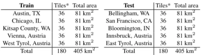
Train Tiles* Total area Austin, TX 36 81 km2 Chicago, IL 36 81 km2 Kitsap County, WA 36 81 km2 Vienna, Austria 36 81 km2 West Tyrol, Austria 36 81 km2
Total 180 405 km2
Test Tiles* Total area Bellingham, WA 36 81 km2 San Francisco, CA 36 81 km2 Bloomington, IN 36 81 km2 Innsbruck, Austria 36 81 km2 East Tyrol, Austria 36 81 km2
Total 180 405 km2
Table 1: Dataset statistics.*Tile size: 15002px. (0.3 m resolution).
areas of the country. Vectorial cadastral records have been re-leased through local or statewide geographic information sys-tem (GIS) websites. We must focus on the zones where such reference data are available in addition to the images.
In the case of Austria, the different provinces have shared images through their respective GIS agencies. We focus, in particular, on Tyrol and Vienna provinces, since open vecto-rial cadastral data are also on hand. We obtained the images through the WMS services provided by the GIS departments2 as well as the associated reference shapefiles.
The original US imagery is provided at either 15 or 30 cm resolution with three or four spectral bands (RGB/RGB-Infrared), depending on the area, and Vienna imagery con-tains three bands (RGB) at a resolution of 10 or 20 cm. We took out the common factor and built our dataset with 30 cm images (average resampling if needed) and the RGB bands.
We consider two semantic classes: building and not build-ing. For this we must extract the so-called building footprints from the cadaster. While there are other classes present in some areas (e.g., trees and roads), the building class is the only one that is consistent across different areas. Roads, for example, are often represented with a line, but it is very often not located at the center of the road and its width is usually not specified. This makes it difficult to derive a pixelwise se-mantic labeling for roads, and is an active research problem itself [5].
Once we selected a number of candidate areas for the dataset, we visually inspected them to assess whether the cadaster is properly aligned with the images. In some re-gions, there are irregular shifts that led us to exclude them (e.g., Seattle and Spokane cities). This may be the result of errors or imprecision in the terrain model used to orthorectify the images, or in the digitization of the cadaster. Note that we have only considered official image and cadaster data sources, ignoring, e.g., OpenStreetMap (OSM) data.
The regions included in the dataset and their distribution into training and test subsets is depicted in Table 1. Note first that the amount of data in each of the subsets is the same. This stresses our goal of properly assessing classification methods that generalize to different areas and images. The regions were split in such a way that each of the subsets contains both European and American landscapes, as well as high-density (e.g., Chicago/San Francisco and Vienna/Innsbruck)
2https://gis.tirol.gv.at/arcgis/services/Service Public/orthofoto/MapServer/
Bellingham Innsburck San Francisco Tyrol Chicago Fig. 2: Close-ups of the dataset images and their corresponding reference data.
and low-density (e.g., Kistap/Bloomington, West/East Tyrol) urban settlements. While aerial images over Tyrol are present in both subsets, they have been obtained at different flights over the country, thus showing different illumination char-acteristics. We have also selected dissimilar images inside some of the groups (e.g., Kitsap County contains tiles from two different flights with very dissimilar characteristics). The reference data was created by rasterizing the shapefiles with GDAL. Fig. 2 shows closeups of the images in the dataset.
We consider two evaluation measures to assess the perfor-mance of different methods on the dataset. First, the accuracy, defined as the percentage of correctly classified pixels. Sec-ondly, the intersection over union (IoU) of the positive (build-ing) class. This is defined as the number of pixels labeled as building in both the prediction and the reference, divided by the number of pixels labeled as building in the prediction or the reference. The IoU has become the standard in seman-tic segmentation [8], since accuracy favors methods that do not take the risk of assigning pixels to minority classes. It is therefore particularly useful in imbalanced datasets such as ours. We compute accuracy and IoU on the overall dataset and for every region independently (e.g., San Francisco).
3. EXPERIMENTS
We experimented with convolutional neural networks on the dataset3. We created a validation set by excluding the first five tiles of each area from the training set (e.g., Austin{1-5}). Such validation set may be useful to assess the conver-gence of the networks or to perform preliminary comparisons of different methods without the need to submit the results to the contest. We first trained a base fully convolutional net-work (FCN) [8], from which we then derived other architec-tures. An FCN is composed of a series of convolutional lay-ers with learnable parametlay-ers, interleaved with subsampling layers. Subsampling increases the receptive field (i.e., the amount of context considered to make a prediction) but at the same time reduces the spatial resolution of the output. Since
3Code and trained models: github.com/emaggiori/CaffeRemoteSensing
Concatenate
Learn to combine features Upsample features Base FCN MLP net. Dense semantic labeling Input image
Fig. 3: MLP network for semantic labeling.
we must naively upsample the classification maps, the result is expected to be overly fuzzy or “blobby”. We train the FCN proposed for Postdam imagery in [9] for 120,000 iterations on randomly sampled patches of our dataset (momentum is set to 0.9, the L2 penalty to 0.0005 and the learning rate to 0.001).
To provide a finer classification, we derived a so-called MLP network on top of the base FCN, as explained in [9]. This network, illustrated in Fig. 3, extracts intermediate fea-tures from the base FCN (which convey information at dif-ferent resolutions and with difdif-ferent receptive fields). The feature maps are upsampled to match the resolution of the highest-resolution maps, and concatenated to create a pool of equally important features. This way, both broad but impre-cise features and local but fine features are considered. To produce the final classification map, a multi-layer perceptron (MLP) takes the pool of features and learns how to combine them. The MLP is simply a neural network with one hid-den layer, applied to every pixel individually. The pretrained FCN mentioned earlier is used to initialize the correspond-ing parameters in the network of Fig. 3, and then the overall system is trained for an extra 250,000 iterations, which takes 50 hours on a single GPU. We start with a learning rate of
Austin Chicago Kitsap Co. West Tyrol Vienna Overall FCN IoU 47.66 53.62 33.70 46.86 60.60 53.82 Acc. 92.22 88.59 98.58 95.83 88.72 92.79 Skip IoU 57.87 61.13 46.43 54.91 70.51 62.97 Acc. 93.85 90.54 98.84 96.47 91.48 94.24 MLP IoU 61.20 61.30 51.50 57.95 72.13 64.67 Acc. 94.20 90.43 98.92 96.66 91.87 94.42
Table 2: Numerical eval. on small validation set. Belling. Bloom. Inns. S. Francisco East Tyrol Overall FCN IoU 44.83 35.38 36.50 44.92 43.69 42.19 Acc. 94.48 94.07 92.97 82.60 95.14 91.85 Skip IoU 52.91 46.08 58.12 57.84 59.03 55.82 Acc. 95.14 94.95 95.16 86.05 96.40 93.54 MLP IoU 56.11 50.40 61.03 61.38 62.51 59.31 Acc. 95.37 95.27 95.37 87.00 96.61 93.93
Table 3: Numerical evaluation on test set.
0.0001, and we multiply it by 0.1 every 50k iterations. The numerical results are summarized in Tables 2 and 3, for the validation and test sets, respectively. We also include the performance of a skip network, which is an alternative way of combining features to refine the predictions of a coarse base FCN (see [9]). Fig. 4 includes close-ups of the classifi-cation on the test set, i.e., on regions never “seen” by the neu-ral network at training time. While the FCN produces fuzzy results, it successfully identifies buildings in varied images. The MLP network provides finer outputs, as confirmed both numerically and visually.
The MLP network reaches about 60% IoU on the entire test set. This means that the output objects overlap the real ones by 60%, as assessed over a significant amount of test data. While there is certainly room for improvement, these values suggest that the current network does generalize well to different cities.
4. CONCLUDING REMARKS
We created a dataset for the semantic labeling of aerial im-ages. This dataset highlights the need for methods that gener-alize to the dissimilar appearance of urban settlements around the earth. Contrary to previous work, the testing is not per-formed over excluded areas of the training surface, but over entirely different cities instead. We cover a wide range of ur-ban densities, on both European and American cities.
Our preliminary experiments with deep neural networks show their satisfactory generalization capability. We hope these results will constitute a baseline for future work and our dataset to be used as a benchmark for comparisons.
5. REFERENCES
[1] Emmanuel Maggiori, Yuliya Tarabalka, and Guillaume Charpiat, “Optimizing partition trees for multi-object segmentation with shape prior,” in BMVC, 2015. [2] Volodymyr Mnih, Machine learning for aerial image
la-beling, Ph.D. thesis, University of Toronto, 2013.
a)
b)
c)
d)
Fig. 4: Visual close-ups on test set. (a) Color input. (b) Ref-erence data. (c) FCN results. (d) MLP results.
[3] Michele Volpi and Devis Tuia, “Dense semantic labeling of sub-decimeter resolution images with convolutional neural networks,” IEEE TGRS, 2016.
[4] Emmanuel Maggiori, Yuliya Tarabalka, Guillaume Charpiat, and Pierre Alliez, “Convolutional neural net-works for large-scale remote-sensing image classifica-tion,” IEEE TGRS, 2016.
[5] Gellert Mattyus, Shenlong Wang, Sanja Fidler, and Raquel Urtasun, “Enhancing road maps by parsing aerial images around the world,” in IEEE ICCV, 2015.
[6] Mathieu Fauvel, Yuliya Tarabalka, Jon Atli Benedikts-son, Jocelyn Chanussot, and James C Tilton, “Advances in spectral-spatial classification of hyperspectral images,” Proceedings of the IEEE, 2013.
[7] Silvia Valero, Philippe Salembier, and Jocelyn Chanus-sot, “Hyperspectral image representation and processing with binary partition trees,” IEEE TIP, 2013.
[8] Jonathan Long, Evan Shelhamer, and Trevor Darrell, “Fully convolutional networks for semantic segmenta-tion,” in CVPR, 2015.
[9] Emmanuel Maggiori, Yuliya Tarabalka, Guillaume Charpiat, and Pierre Alliez, “High-resolution seman-tic labeling with convolutional neural networks,” arXiv preprint arXiv:1611.01962, 2016.