Extracting structured models from raw scans of manufactured objects : a step towards embedded intelligent handheld 3D scanning

(1)

Extracting Structured Models From Raw Scans of

Manufactured Objects:

A Step Towards Embedded Intelligent Handheld 3D Scanning

Thèse

Zahra Toony

Doctorat en Génie Électrique Philosophiæ doctor (Ph.D.)

Québec, Canada

(2)

(3)

Résumé

La disponibilité de capteurs 3D rapides et précis a favorisé le développement de différentes applications dans les domaines de l’assemblage, de l’inspection, de la conception assistée par ordinateur (CAO), de l’ingénierie inverse, de la construction mécanique, de la médecine, et du divertissement, pour n’en citer que quelques-unes. Alors que les caméras 2D capturent des images 2D de la surface des objets, soit en noir-et-blanc, soit en couleur, les caméras 3D fournissent des informations sur la géométrie de la surface d’un objet. Aujourd’hui, les caméras 3D nouvellement introduites peuvent acquérir l’apparence et la géométrie des objets en même temps.

La popularité et la disponibilité de ces modèles 3D a ouvert de nouveaux champs d’inté-rêts, comme segmentation de modèles 3D, la reconnaissance du modèles 3D, l’estimation des paramètres de modèles 3D et même la modélisation 3D.

Dans ce projet, nous visons à faire une reconnaissance intelligente des différentes parties (pri-mitives) d’un objet 3D. À cette fin, nous préparons d’abord une base de données de primitives de CAO 3D (i.e., plans, cylindres, cônes, sphères et tores). Ensuite, en utilisant les algorithmes de segmentation, les objets complexes sont décomposés en leurs primitives et, en utilisant des techniques de reconnaissance des formes, un descripteur est associé à chaque primitive et, enfin, un classificateur est formé pour apprendre les propriétés des primitives. Le manuscrit étudie différentes méthodes liées à ces défis. Une étape supplémentaire est également proposée dans ce projet, par l’estimation des paramètres des primitives et la génération de primitives de CAO, qui complète l’ensemble du processus d’ingénierie inverse.

(4)

(5)

Abstract

The availability of fast and accurate 3D sensors has favored the development of different appli-cations in assembly, inspection, Computer-Aided Design (CAD), reverse engineering, mechan-ical engineering, medicine, and entertainment, to list just a few. While 2D cameras capture 2D images of the surface of objects, either black-and-white or color, 3D cameras provide informa-tion on the geometry of an object surface. Today, newly introduced 3D cameras can acquire the appearance and geometry of objects concurrently.

The popularity and availability of such these 3D models has opened new fields of interests, such as 3D model segmentation, 3D model recognition, estimation of 3D models’ parameters and even 3D modelling.

In this project, we aim at recognizing different parts (primitives) of a 3D object, intelligently. For this purpose, we first prepare a database of 3D CAD primitives (i.g. planes, cylinders, cones, spheres and, tori). Then using segmentation algorithms, the complex objects are decom-posed into their primitives and, by utilizing recognition techniques, a descriptor is extracted and associated to each primitive and, finally, a classifier is trained to learn the properties of primitives. The manuscript investigates different methods related to these challenges. An additional step is also proposed in this project which estimates the parameters of primitives and generate the CAD primitives that completes the whole process of reverse engineering.

(6)

(7)

List of tables

2.1 Generated Models in the GPrimDB. . . 52

3.1 Min, max, and mean values of c value introduced in Algorithm 2.4. . . 96

3.2 Partial and complete torus models parameters error . . . 106

3.3 Training the classifier with or without the skewness value. . . 109

3.4 The best selected pair of C and γ at each fold during training the classifier with the skewness value and 202 bins. . . 109

3.5 Training the classifier with different number of bins in the histogram. . . 110

3.6 The error values of the estimated parameters for the first CAD model . . . 114

(10)

(11)

List of figures

1.1 How to create a 3D model. . . 8

1.2 Accuracy of different most common active sensors . . . 9

1.3 Range data samples [197] . . . 10

1.4 3D shape acquisition and modelling techniques . . . 12

1.5 Comparison of the method presented in [103] to previous segmentation approaches 16 1.6 A comparison between manual boundary detection and the output of the algo-rithm presented in [9] . . . 17

1.7 Spin image . . . 24

1.8 The process of supervised machine learning [112]. . . 26

2.1 Diagram of the method proposed in the thesis. . . 32

2.2 1-ring face neighbourhoods . . . 37

2.3 The result of Sun’s method [183] for the Fandisk model. . . 38

2.4 Normal direction of a 3D model . . . 43

2.5 A color-coded representation of similarity matrix values for two 3D models . . . 43

2.6 3D-NCuts segmentation of a 3D model . . . 44

2.7 3D-NCuts segmentation with different similarity matrices . . . 47

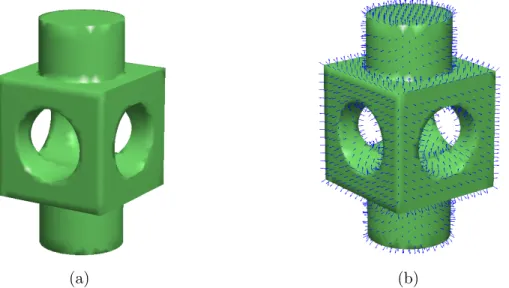
2.8 3D principal primitives with their normals on the model and on the Gaussian sphere. . . 49

2.9 Comparing the result of fitting a plane on the normals mapped on the Gaussian sphere using mean and median . . . 51

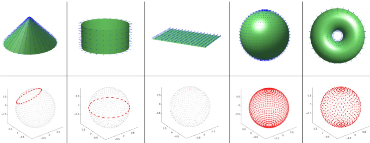
2.10 Typical unit Gaussian sphere for all types of primitives (full and partial) . . . . 53

2.11 Different parameters used for analyzing the Gaussian sphere. . . 54

2.12 Illustration of normals distribution on the Gaussian sphere with respect to the PCA plane . . . 57

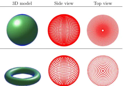
2.13 The dispersion of normals on the Gaussian sphere for spheres and tori . . . 59

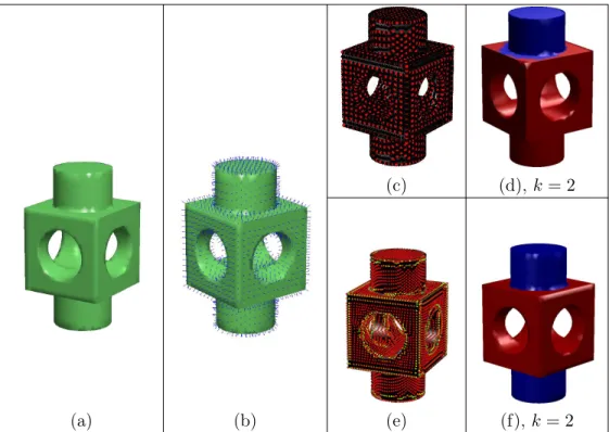
2.14 Triangulations of the CAD models and their decimated models with associated results of voting on the Gaussian accumulator . . . 60

2.15 The difference between regular voting of the Gaussian accumulator in compa-rison with the proposed Density Weighted Voting approach . . . 62

2.16 The different plots of the Gaussian accumulator’s statistical moments . . . 63

2.17 The Skewness value of the Gaussian accumulator for 100 spheres and 100 tori. . 63

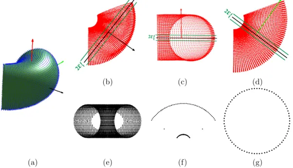
2.18 The sorted histogram of Gaussian accumulator values for 10 spheres and 10 tori 64 2.19 The parameters extracted for plane, sphere, cylinder, cone, and torus . . . 65

2.20 Extracting the parameters of a real scanned plane . . . 66

2.21 Extracting the parameters of a cylinder . . . 69

(12)

2.23 Extracting the parameters of a torus . . . 72

2.24 Finding the correct direction vector for a partial torus . . . 72

2.25 Diagram of the distances to the plane . . . 74

2.26 Finding the parameters of the circles for a partial torus . . . 75

3.1 A sample of each type of primitive as well as partial models. . . 82

3.2 Denoising Fandisk model Corrupted with zero mean Gaussian noise with stan-dard deviation σ = 0.25 of mean edge length . . . 83

3.5 Denoising Bunny model Corrupted with zero mean Gaussian noise with stan-dard deviation σ = 0.25 of mean edge length . . . 84

3.8 Removing outliers from the normals of a real scanned model . . . 85

3.9 Comparison of the performance of 3D-NCuts to other segmentation methods . 87 3.10 The result of the proposed 3D-NCuts segmentation method in comparison with the method proposed by [206] . . . 88

3.11 The result of the proposed 3D-NCuts segmentation approach in comparison with the method proposed by [206] on real scanned data. . . 88

3.12 The result of the proposed 3D-NCuts 3D segmentation approach in the presence of noise . . . 89

3.13 More results of the 3D-NCuts segmentation approach . . . 89

3.14 3D-PIC Segmentation of a 3D model with different number of clusters. . . 90

3.15 Comparison with the method proposed by [206] . . . 91

3.16 The result of the proposed 3D-PIC segmentation approach in the presence of noise . . . 92

3.17 3D-PIC segmentation of real 3D models. . . 93

3.18 More segmentation results achieved by 3D-PIC approach. . . 93

3.19 Comparison between feature extraction methods for four principal primitives . 97 3.20 D2 descriptor for the principal primitives and their partial models. . . 98

3.21 Partial cylinders and cones on the Gaussian sphere . . . 98

3.22 The result of the Gaussian accumulator for partial spheres and partial tori as well as complete spheres and tori with different number of cells . . . 99

3.23 Primitive detection using our approach for the segments of two complex models. 100 3.24 Primitive detection using our approach for real scanned models. . . 101

3.25 Comparison of sphere parameters between ground truth values, our method (PGP2X), Attene’s method and LSGE . . . 103

3.26 Comparison of cylinder parameters between ground truth values, our method (PGP2X), Attene’s method and LSGE . . . 104

3.27 The difference between ground truth values for height and centre of cylinders and results obtained by our method (PGP2X) . . . 105

3.28 Cone parameters comparison between ground truth values, our method (PGP2X) and Attene’s method . . . 107

(13)

3.29 Comparison of partial Cone parameters between ground truth values, our

me-thod (PGP2X), and Attene’s meme-thod . . . 108

3.30 The process of removing the plane supporting all primitives . . . 111

3.31 The result of the Part-to-CAD process for the first CAD model. . . 112

(14)

(15)

Acknowledgments

First and foremost I would like to express my deepest appreciation to my supervisor, profes-sor Denis Laurendeau, director of the Computer Vision and Systems Laboratory (CVSL) in Laval University. He has been supportive since the days I began working on this project. He has supported me not only by providing a research assistantship, but also academically and emotionally through the road to finish this thesis.

Thank you to my co-supervisor, professor Christian Gagné who provided me with a special opportunity to work with him. I really appreciate all the time, help and effort, he has invested in me and my project. Especially, I would like to acknowledge his guidance and support throughout these past few years both in academic and non-academic situations.

With all my sincere feelings, I would like to extend my gratefulness to my husband, Peyman, who never stopped believing in me. I dedicate this thesis to him. Many thanks to Denis Ouellet for his valuable academic advice. Special thanks go to my friends in CVSL Lab, Somayeh Hesabi and Trung-Thien Tran, for their explicit help and support and to Annette Schwerdtfeger for proofreading all manuscripts resulting from this thesis.

I gratefully acknowledge FRQNT post-graduate scholarship and NSERC-Creaform Industrial Research Chair for their support of my research program ; this work would not have been possible without their support.

(16)

(17)

Introduction

The vision sense has an important role in life. It allows people to infer spatial properties of the environment which are essential to perform crucial tasks. Even simple living organisms are capable of “remote” and “non-contact sensing” of their environment. Information which comes from sensing is processed in the brain in order to build a representation of the world which enables people to evolve in the environment while performing different actions such as recognizing objects, detecting danger, executing various tasks, etc. [132].

A collection of instruments which obtain an estimation of the environment’s geometrical pro-perties by transforming light intensity is called a vision system [132]. As an example, the human vision system captures light from the environment on the retina and the information is sent to the brain for further processing of transforming the light intensity to the 3D model of the scene [132]. Recently, artificial vision systems have been developed to perform such measurements in order to produce three-dimensional representation of a scene or environment [132].

Sensing technology, especially in computer vision, has been influenced by different factors such as innovative sensing electronics and increase of computer processing power which can now meet the requirements of real-world applications. During the last years, vision sensors have evolved from being sophisticated lab equipment to “practical” and “commercial devices” [204]. A vision sensor is usually under the complete control of the user (except maybe for low-level tasks such as gain control and focus), but intelligence is to be added to the sensors to support data capture. An intelligent sensor is able to modify its internal processes to optimize the act of collecting data from the environment (external world) and then communicating with the host system [23]. There are many applications of intelligent sensing in industry and robotics. In the early 1980s, the availability of precise 2D and 3D cameras has opened a new field of computer vision, 3D image acquisition and processing [16]. Nowadays, this field has found many different applications such as assembly, inspection, Computer-aided Design (CAD), reverse engineering, mechanical engineering, medicine, and entertainment.

Standard 2D cameras produce 2D appearance images of the surface of objects, in either black-and-white or color, while 3D cameras rather provide information on the geometry of the object

(18)

surface. Today, some 3D cameras can acquire both the appearance and geometry of objects concurrently. This results in many 2D processing approaches applied on 3D images : 3D mesh compression [29; 97; 211], 3D skeleton extraction [10; 162; 219], 3D object recognition [90;

104; 142; 168], and 3D segmentation [116; 126; 206] are instances of such extensions of 2D approaches to 3D.

3D sensing is thus becoming popular and can be applied to a large variety of applications in mechanical engineering, neuroscience, astrophysics and also other fields and industries inclu-ding entertainment, cultural heritage preservation, geo-exploration, architecture, and urban modeling [19]. To name just a few practical applications, we can mention, face detection [25], 3D plant analysis [151], and medical applications [108]. For instance, 3D scanners are used in the medical domain to capture the 3D models (shapes) of the patients in orthotics and dentistry. A CAD (Computer Aided Design) software is then used to design and construct the orthotics, prosthesis, or dental implants.

The long-term goal of the currect project is to use a 3D handheld sensor (and the data it produces) in order to recognize the type of components (primitives) of complex objectsduring the scanning process instead of a posteriori. In addition, intelligence would be embedded in the sensor so, i) it can help the user to become more efficient in the scanning process and ii) it can ease scanning of similar parts every time a sample is captured. Reducing the workload of sensing modules and the overall algorithms is the essential role of learning algorithms which extract relevant information from the sensing components and transmit the useful information to the data processing modules.

The thesis explores the steps that we believe would be required by the next generation of 3D sensors to produce a CAD model while the sensing process is performed. The steps for embedding this type of intelligence in the next generation of sensors are described in figure 2.1. In this thesis, these steps are executed a posteriori of the scanning step itself because the current generation of sensors do not provide enough processing capabilities to achieve these steps during scanning.

For reconstructing the geometry of an object from 3D data, it is required that many views of this object be acquired from different positions and orientations in space through successive overlapping measurements. The overlapping views are used for registration (i.e., alignment), integration, and reconstruction of a mesh of the 3D object. In our case all the aforementioned steps of the process are done by a Creaform handheld scanner. Usually, in a standard non-intelligent scanning process, the user decides arbitrarily whether or not enough data has been collected in order to build a reliable CAD model. This leaves some randomness in the scanning process as some parts, such as planes, may be oversampled while others (with large curvature) may remain undersampled.

As an application, our project can be used to add intelligence at the scanning step such that

(19)

it can help the user to decide when enough data has been acquired to identify the different parts of the object and decide where new scans should be obtained. In order to reconstruct the CAD model, some recognition tasks are needed, which in turn require efficient mesh representations known as “shape descriptors” which can describe shapes locally or globally [49]. This means that according to some basic hypotheses on the shape of the surface of the scanned object, e.g., general convexity, curvature, scale-, orientation- (or both) invariant features [26; 49;111; 130; 213], an approach should be developed to propose a trajectory to the user for the displacement of the sensor over the scanned object in order to collect the right amount of data for producing the CAD model. Such descriptors are also useful for extracting basic features of the surface composing the object.

The embedded intelligence could also be used for recognizing a given region that needs to be measured more accurately or a region where given measurements need to be acquired depending on the location on the surface. Since it is requested to recognize the 3D object parts gradually while scanning, producing high-level descriptions which can be used in CAD models are highly desirable. This method should take into account the data acquired so far, the desired precision of the model to be built, the uncertainty of the self-positioning of the sensor, and the optimization of the sensor displacement for the operator (time efficiency and user-friendliness).

In order to produce accurate CAD models from raw 3D data, removing noise from the data can also be an important pre-processing step. 3D scanning sensors can produce either range images or unstructured point clouds. Both types of data are subject to noise from various sources, so removing the noise from the 3D model while preserving its features is very important especially when extracting the features. Some successful methods like bilateral mesh denoising [66], mesh denoising by quadratic error metric [200], or even feature-preserving mesh denoising schemes [183;202] have been proposed. The latter try to remove noise while preserving sharp features in the model that are usually weakened by the smoothing process. After such a denoising procedure, feature extraction for recognizing object’s parts should be more efficient and robust.

0.1 Problem description and objectives

The proposed method is described as follows : a database of 3D geometric primitives is prepared and their features are then extracted. A new feature descriptor concept is proposed for this purpose. A classifier is then trained on the database in order to learn the features of the primitives for a recognition task. After the scanning process, when enough data is acquired to recognize a part, a denoising technique could be used which depends on the amount of noise captured by the 3D scanner, and then a segmentation approach is applied to separate primitives if more than one primitive has been scanned so far. Then the features of each

(20)

segment are extracted and their primitive type is recognized by the trained classifier. If there is enough data, the parameters of the primitive are estimated afterwards and that primitive can be reconstructed from the database without further scanning. The scanning can be continued to obtain more accurate measurements or to complete other parts of the model (object). As mentioned before, the denoising approach can be used before extracting the feature descriptor in order to increase the accuracy. It should be mentioned that all 3D objects that are used in the framework presented in the thesis are 3D triangular meshes.

The contribution of this thesis are listed as follows :

1. Presenting a new database of 3D geometric primitives including planes, cones, cylinders, spheres, and tori as well as partial models of the latter four primitives (GPrimDB). These geometric primitives are formatted as 3D triangular meshes to the best of our knowledge, such a database does not exist,

2. Presenting a new feature descriptor (Gsh+s) in order to extract salient properties of 3D geometric primitives for recognition purpose. In order to extract one of the features for the descriptor, a new concept of Gaussian accumulator is presented in this thesis, 3. Tuning a classification method for the train-and-test process of recognizing 3D geometric

primitives. Since the input data is available with their desired class labels (type of primitives), a supervised learning approach is exploited,

4. Proposing two 3D segmentation approaches, 3D Power Iteration Clustering (3D-PIC) and 3D Normalized Cuts (3D-NCuts), in order to select the one suited best for our application. These methods separate different primitives of a scanned object if more than one primitive is present,

5. Improving existing approaches for the estimation of descriptive parameters of cylinders, cones and, spheres,

6. Proposing a new method to estimate the parameters for a torus model, 7. Proposing a new algorithm to plot CAD planes and cones,

8. Adapting a noise removal method to our application and,

9. Modifying and adapting a point cloud noise removal approach to our application of removing outliers from the set of surface normals.

The approach proposed in this thesis allows the improvement of the following tasks :

X So far, the CAD model of an object is usually produced after scanning and the amount of scanned data must be set intuitively by the user. The long-term goal of this project is to produce a CAD model while scanning the part with the right amount of data, in order to reduce capture time and increase user efficiency. In the present thesis, this goal is achieved as a post-processing implementation since current sensors do not support a real-time implementation.

(21)

X By scanning the object, a high-level description of this object and, therefore, its CAD model can be produced. So, the framework proposed in the thesis can be used in reverse engineering, in the case of producing complex CAD models, by building the CAD model of each disassembled part to finally assemble the complex CAD model.

X Our method also aims at providing the measurements of the identified CAD primitives along with their location on the resulting CAD model. This step completes the process of reverse engineering.

X If CAD models are outdated, our intelligent 3D scanning process could provide an up-dated version by scanning the real object again and updating its structure. It can also be used for replacing missing or older parts of a CAD model.

X While scanning an object, its CAD model could be provided by an intelligent sensor for comparing the scanned object with a model known a priori.

0.2 Illustrative example of the proposed intelligent scanning

procedure

Suppose that there is a real 3D object for which we want to build the 3D computer model using a scanner. With a regular 3D scanner (i.e., one without embedded intelligence) it is difficult for the user who may not be an expert in 3D to assess how many data points should be captured on each part of the object. The object must be scanned until the user feels that enough points have been collected to build a 3D digital model (often a triangular mesh). The goal of this thesis is to introduce a framework which will allow the development of a scanner which obtains a 3D CAD model immediately once scanning is complete. This requires that intelligence be embedded in the scanner in order to guide the user during scanning and to avoid unnecessary scanning. The scanner we propose to be developed should work as follows. Given a 3D object, one starts to scan the object and when enough data has been captured on a given part, the system informs the user to stop scanning and to continue scanning another part. This helps to save time and make the scanner easier to operate by a non-specialist. Such an intelligent scanner could even guide the user on which direction to scan in order to get better 3D models faster (this is not part of the current thesis but the steps proposed in the framework could be used in such an intelligent sensor). We propose to produce the CAD model of the 3D object at the end of the scanning process. The CAD models can be used by software tools for further processing such as forward/reverse engineering.

Embedding intelligent algorithms into the scanner makes it easier to use and help to guide users who are not specialists in 3D scanning. For this purpose, first, we need to prepare a database of 3D objects that can be used for 3D object classification and recognition. Now, during the scanning of an object a hidden process is executed : the scanned model is segmented into its different primitives, if there is more than one. Then a descriptor of the features of the

(22)

segmented primitive is extracted in order to find its similar primitive in the database. To find the similar primitive, a classifier which is already trained on the database is used. The parameters of that primitive are also estimated and then a primitive of that type with the same parameters is extracted from the database. By doing so, additional scanning is not required and the user can then start scanning another part of the object. However if the scanned part does not exist in the database it is added to it once scanning is over. The database is thus augmented dynamically while scanning new objects.

As a scan of an object is corrupted by noise, a 3D denoising method is applied on the collected data while preserving sharp features (like edges and corners). Denoising and feature extraction are performed during scanning. A major feature of the framework proposed in the thesis is that the CAD models of the scanned 3D objects could be available immediately after the scanning procedure. The 3D sensor has thus the embedded intelligence needed to produce the CAD model of any 3D object in a period of time close to scanning time.

The thesis thus provides an explanation of the functionalities that need to be included in the next generation of handheld 3D sensors in order to embed intelligence in the scanning process.

(23)

Chapter 1

Literature Review

In this chapter, we present an overview of the different concepts at the centre of the thesis and then for each concept, a review of most recent and the most important methods is considered.

1.1 3D modelling

The process of creating a three-dimensional computer model of an object is defined as 3D modelling. 3D modelling has different meanings in computer vision and computer-aided-design (CAD). In computer vision, a 3D model is created from range data, but in CAD, the 3D model is built based on computer-generated geometric primitives. When the 3D model is built through the acquisition of range data, the process is called real-time 3D modelling [197]. Creating a 3D model from a real object is composed of the following steps : acquisition, registration, integration or reconstruction, and visualization (see figure 1.1). A modelling step, shown in gray shade, always runs before registration because a local low-level model (e.g. triangular mesh) is often used for registration instead of raw data. In interactive modelling, the above steps are part of a loop that integrates new data as it is acquired.

1.1.1 Acquisition

3D cameras capture images that collect information on the geometry of an object. There are different types of 3D cameras (active or passive) using various technologies for image acquisition and data production. Active 3D sensors use an artificial illumination which can be either a spatially coherent light source (e.g. laser) or an incoherent one (e.g. halogen lamp). They can produce dense 3D maps with low ambiguity by projecting a point or pattern on the surface of the object [53]. Since an active sensor uses artificial light, it is able to generate a model of an object geometry even when its surface is featureless [53].

The three most frequently used principles in commercially available active sensors are “time-of-flight ”, “interferometry ”, and “triangulation” [53]. The accuracy of the different types of

(24)

Figure 1.1 – How to create a 3D model.

active sensors as a function of operating distance is shown in figure 1.2 [53]. As seen in this figure, the coverage range (operating distance) of each method is different. To exploit the basic principle of the time-of-flight method, different approaches have been proposed [2;13;93]. In pulse-based time-of-flight, the time between light pulse emission and light detection on a sensor is computed. So, the distance between the sensor and points on the surface is computed based on the time traveled by the light pulse and light speed. In the phase-based time-of-flight approach, instead of a pulse, a continuous wave (e.g. sine) is used and the distance is computed based on the phase shift between the received and emitted signals [64].

The superposition of two light beams is known as Interferometry while the laser beam is split in two paths with known length and unknown length [53]. Because of path length differences between light beams, there is a phase difference between them. They are then combined together, superposed, and the interference pattern is observed by the photo-detector. The resulting depth measurement depends on the path difference [53].

In triangulation methods, the reflected pattern is observed by the camera. Knowing the dis-tance between the camera and the source and the orientation of the source, the coordinate of points on the surface of the object can be computed in the camera reference frame by triangu-lation. To find more details on 3D active sensors the reader is referred to [133] and to a recent article [53].

In Passive 3D sensors no external light source is used and the 3D information on the scene which is illuminated by an ambient lightening is recovered by the sensor [167]. Passive 3D imaging systems are classified in two categories : single-view and multiple-view [167]. In

(25)

Figure 1.2 – Accuracy of different most common active sensors as a function of operating distance [53].

multiple-view approaches, several views of the scene are acquired using one of the two fol-lowing methods : “stereo” (multiple cameras at the same time) and “structure from motion” (one moving camera at different times) [167]. The coordinates of surface points are computed by triangulating the rays produced by acquired images via two or more cameras [167]. In passive single-view approaches, the information from the scene is obtained from sources like “shading”, “texture” and “focus” that are also called “shape from shading”, “shape from texture” and “shape from focus” respectively [167]. For more details on passive technology refer to [167]. Depending on the approach used, 3D cameras provide different types of range data. Range data is a set of captured 3D points which describes physical positions of the points on the object’s surface. Classification of range data based on connectivity information was investigated for three categories of data [197] :

1. Unorganized sets of points or point clouds : this category does not show any specific spatial organization or connectivity information between points and the points are stored in random order (figure 1.3a). Such images are often provided by techniques such as stereo vision or LIDAR.

2. Range curves or scans : this class contains set of points measured along curvilinear paths and each point has two neighbours except the two end points ; the connectivity between neighbouring points on a scan is generally available (in smooth areas of the surface) but the connectivity of points on different scans is not be available automatically

(26)

(a) (b) (c)

Figure 1.3 – Range data samples [197] : (a) unorganized sets of points ; (b) range curves ; (c) range images.

(figure 1.3b). This type of image often results from the use of a light stripe scanned over the object during data acquisition by an active 3D camera.

3. Range Images, surface patches, or raster images : this group is structured as a set of points organized in parametric grids. Each point is connected to its neighbours which results in a surface (e.g. triangulated mesh), see figure 1.3c. The connectivity, 4-neighbour or 8-neighbour, is directly available from the image.

For more information about range sensing technologies, the reader is referred to [16].

1.1.2 Registration

Viewing an object completely from a single viewpoint, regardless of the type of 3D sensor, is not possible. To cover the entire surface of an object, it needs to be observed from different views in different positions and orientations. This can be achieved by moving either the object or the sensor (or sometimes both) [197]. The sufficient number of views depends on both the geometry of the object and the sensor and also the accuracy of reconstruction that is needed. When moving the object or the sensor to observe different viewpoints of the object, the location of the sensor relative to the object should be known to align range data from all viewpoints in a single and global reference frame. The task of finding the rigid (or nonrigid) transformation to express the data collected in local reference frames in a common global reference frame is called Registration. Registration is a complex problem which has received a lot of attention in 3D vision research. Many approaches have been proposed to find the rigid transformation automatically and align the range data. Iterated-Closest-Point (ICP) [14] is one of the most famous methods. The range data which is acquired from different points of view generally overlap. the overlapping parts contain redundant data. This redundancy is useful in solving the registration problem by automatic alignment methods [197]. For some other techniques,

(27)

the transformation can be estimated by an external positioning device such as the C-track photogrammetric system of the MetraScan 3D scanner [44].

A document has been prepared recently on image registration methods which contains more details [80].

1.1.3 Reconstruction

At this step, we assume that 3D data has been acquired in enough views to cover the whole surface of an object and then registration has been performed with enough accuracy to allow reliable reconstruction. The surface reconstruction consists of converting the aligned views into a continuous surface representation that is ideally a virtual replication of the real object [197]. Some of 3D reconstruction methods are presented in figure 1.4.

The first method, based on the shading on a surface (figure 1.4a), provides a lot of information about the overall surface shape and local orientation [185, Ch. 12, p. 505]. This method is especially useful in photometric stereo applications (when lights illuminating the scene from different directions can be turned on and off separately). When we look at an object, we can obviously infer its shape just from shading variations which result from brightness change due to surface normal variation on the object [185, Ch. 12, p. 505]. The shape-from-shading approach is in fact the task of recovering the model (shape) of an object using this variation in intensity [185, Ch. 12] which is a classical problem in computer vision [87]. There is a complete survey about shape from shading methods in [220] which reviews and compares different approaches.

Variations in foreshortening of regular patterns provide suitable information about local sur-face orientation (figure 1.4b) [185, Ch. 12]. Some pre-processing steps are required to implement shape from texture algorithms including the extraction of repeating patterns, or the measu-rement of local frequencies for obtaining local affine deformation of the pattern as well as the steps needed to obtain local surface orientation [185, Ch. 12]. To find more details on each pre-processing step the reader is referred to [17;76;91;129;135;205].

The amount of blur in an image can be used to estimate the depth. Blurriness increases as the object’s surface moves away from the camera’s focusing distance. So, focus is a strong way to obtain scene depth, see figure 1.4c, especially when two or more images with different focus settings are used [185, Ch. 12].

As presented in figure 1.4d, 3D shape can be reconstructed using active illumination methods such as light stripes (figure 1.4d) or time-of-flight range finders, see [185, Ch. 12, p. 505] for more details. These methods, or even passive stereo techniques, provide partial models of objects which can then be merged into more organized 3D models (figure 1.4e) [185, Ch. 12]. These methods can be used for applications aiming at building accurate models of cultural

(28)

heritage objects or structures (e.g. buildings) [185, Ch. 12].

(a) (b) (c)

(d) (e) (f)

(g) (h) (i)

Figure 1.4 – 3D shape acquisition and modelling techniques [185, Ch. 12] : (a) shaded image [220] (b) texture gradient [76] (c) real-time depth from focus [144] (d) scanning a scene with a stick shadow [21] (e) merging range maps into a 3D model [48] (f) point-based surface modelling [153] (g) automated modelling of a 3D building using lines and planes [203] (h) 3D face model from spacetime stereo [218] (i) person tracking [179].

When prior knowledge is available on the object to be reconstructed, 3D modelling will be more efficient if Model-based reconstruction is used [185, Ch. 12]. Three common examples are shown in figure 1.4 : architecture (figure 1.4g), heads and faces (figure 1.4h), and whole human body (figure 1.4i).

(29)

After modelling the 3D shape of an object or a person, the last stage is to collect texture information that is mapped onto the 3D model geometry to describe the object’s appearance. The simplest way to achieve texture mapping is to consider a separate texture map for each triangle of the 3D shape [185, Ch. 12] or to use a 3D sensor that captures appearance in-formation simultaneously with 3D data [45]. More information on accurate texture mapping approaches can be found in a recent and complete survey [185, Ch. 12].

1.1.4 Visualization

The information visualization field has started in the 1980s and has popularized rapidly in the marketplace [56]. Nowadays, expensive graphic workstations or high-end graphics cards make real-time and advanced interactive graphics possible in “animation”, “space exploration” and “visual effects in 2D and 3D formats”, information visualization technologies are widely available [56]. Since model visualization is out of the scope of this thesis, this topic is not developed further.

1.2 3D segmentation

One of the challenges in shape processing and understanding is to segment a 3D object into meaningful parts [146]. This implies segmenting a 3D shape, not based on distances, but rather based on its geometric properties to obtain a result close to the manual segmentation perfor-med by a human. Many applications, such as object recognition, modelling, or compression depend on meaningful segmentation [103]. In some other applications, segmentation is used to label specific parts of the 3D shapes. Most of these segmentation approaches are performed manually. Segmenting shapes manually leads to various results, e.g. for a human body, one user could distinguish “arm”, “leg”, and “head” from each other while another user could rather discriminate each part of body as a separate segment [103].

3D segmentation can be implemented on two different types of 3D models : 3D meshes and 3D point clouds. In the following, a review of the methods proposed in each category will be presented with the focus being directed toward mesh segmentation approaches.

1.2.1 Mesh segmentation approaches

In reference [170], algorithms for 3D mesh segmentation are classified into five groups, while in reference [1], a more detailed classification of 3D mesh segmentation methods identifies twelve groups : “Region growing”, “Watershed-based”, “Reeb graphs”, “Model-based”, “Skeleton-based”, “Clustering”, “Spectral analysis”, “Explicit Boundary Extraction”, “Critical points-based”, “Mul-tiscale Shape Descriptors”, “Markov Random Fields” and “Direct segmentation”.

Each of these groups can perform the segmentation in two main ways : surface-based and part-based. A surface-based 3D mesh segmentation method attempts to segment a model into

(30)

different regions that express separate surfaces of the 3D model such as planes or cylinders. On the other hand, a part-based approach attempts to segment a mesh into meaningful volumetric parts [1]. The more relevant methods will be reviewed in the following but in order to find more details on each category, the reader is referred to [170;1].

The theory of spectral graphs was introduced by [41] and was then applied on image segmen-tation by [176] as Normalized Cuts (NCuts). 3D spectral analysis approaches first define a similarity matrix on the data, based on properties of mesh connectivity, geometry, etc. Then, a Laplacian matrix is computed based on the defined similarity and its eigenvectors are de-termined in order to segment the 3D model. Since the Laplacian matrix and eigenvectors are found based on the similarity matrix, the most important step of spectral analysis methods is how the similarity is defined such that good segmentations are then obtained.

In 2004, Liu and Zhang [126] applied spectral analysis on 3D models. They defined the si-milarity matrix as the likelihood that faces belong to the same segment. In order to prevent merging faces with different concavities, they used the distance matrix presented in [178;106]. They constructed the normalized similarity matrix on the faces and then identified the k ei-genvectors with the largest associated eigenvalues for further processing. Finally, they applied k -means on the processed eigenvectors. They segmented a model by emphasizing concavities, which sometimes resulted in segmenting unmeaningful concavities [1]. Another method [216] used the same similarity matrix with recursive spectral cut and Nyström approximation [68], which offered the opportunity of defining a partial similarity matrix. The extracted eigen-vectors are then used in a line search algorithm to find the most prominent cut in order to segment the 3D model. In [127], a spectral analysis algorithm based on spectral embedding and 2D contour analysis was proposed. The 3D model was projected into the 2D domain in order to apply contour analysis. The algorithm required that some parameters be selected, and was likely to fail in the presence of noise.

Some other types of segmentation algorithms are based on region growth. In these methods, a seed point is first selected and a region is then grown around them, in order to find final regions. This often leads to over-segmentation [221]. Watershed-based approaches are also subject to over-segmentation of the 3D models [1].

Some other methods, such as Randomized Cuts [78], combine the advantages of using different segmentation methods to benefit both random and non-random features. In order to segment a 3D model, Golovinskiy and Funkhouser [78] generate a pool of segmented parts using different approaches such as k -means [178], hierarchical Normalized Cuts, and Min Cuts. Afterwards, based on the reputation of each edge on a segmentation boundary, they define a “partition function” on edges. “Consistent cuts” are then found and the model is segmented through these cuts.

For the k -means approach, the number of clusters is set and the k -means clustering algorithm

(31)

is repeated several times in order to generate different segmentation results. In the hierarchical Normalized Cuts method, the algorithm starts with every face in a separate segment and then tries to merge them based on an area-normalized cut cost function until the desired number of clusters is obtained. The cost function is the sum of the cut costs of segments divided by their areas. This cost function, called modified version of Normalized Cuts, is exploited instead of using only the cost of all edges in a segment which is utilized as Normalized Cuts in [176]. This algorithm is repeated to obtain different results. Finally, in the Min Cuts approach a set of k seeds is selected and a weight value is defined for each edge in order to maintain the cuts at a large distance from the seeds. This method is also repeated to provide more different segmentation results.

In [114] a random walk approach is implemented in order to achieve mesh segmentation. The authors compute the dual graph of the mesh and select the seeds automatically. The number of seeds is greater than the desired number of clusters. They then try to associate each face with a seed with the highest probability which results in an over-segmented mesh. A hierarchical method is then applied to merge the similar segments based on the length of common boundaries and overall perimeter of adjacent segments [36].

The hierarchical fitting primitive approach that is proposed in [3] considers each face as a segment and starts to merge faces until the desired number of clusters is obtained. At each iteration, a geometric primitive such as a plane, sphere, etc. is fitted to each pair of faces and the best fitted pair is then merged as a segment [36].

Another approach which is called Shape Diameter Function (SDF) [173] defines a scalar func-tion for every face of the mesh and produces a 1-D histogram. Then, a Gaussian Mixure Model is applied on the histogram to fit k Gaussian functions on each face and determine the pro-bability of assigning faces to each SDF cluster. Finally an alpha-expansion graph-cut method is used to minimize an energy function in order to find the appropriate segmentation. This method determines the number of clusters automatically [36].

Recently, a mesh segmentation method for CAD models was presented in [206]. At first, the CAD model is clustered into sparse and dense triangular regions. Using the Gauss map of triangular faces and the Hough transform, sparse triangular regions are separated into planar regions, cylindrical regions and conical regions. Dense triangular regions are also segmented by a mean-shift operation which is applied on the mean curvature field of mesh surfaces. One of the problems of this method is that it deals poorly with planar regions composed of non-uniform parts combining sparse and dense triangulations.

1.2.2 Point cloud segmentation approaches

An unstructured set of 3D points forms a 3D point cloud that is collected by scanners such as Light Detection and Ranging (LIDAR), laser range finder or, Microsoft Kinect [83]. One of

(32)

Figure 1.5 – Comparison of the method presented in [103] to previous segmentation ap-proaches, for chairs, octopuses, and quadrupeds. In each line, the training meshes are shown in the first column and the other columns are test meshes for different methods : (a) [103]’s method, (b) average human segmentation from the Princeton Segmentation Benchmark, (c) Consistent Segmentation [79], (d) Shape Diameter [172], (e) Randomized Cuts [78], with num-ber of segments defined as the average numnum-ber of segments in the category. The method pro-posed in [103] also provides labels in addition to segmentation but the other schemes only perform segmentation.

the main reasons that the point clouds are still used is that they do not include any further interpretation of the scene or the model [83].

Based on what is presented in [83], point cloud segmentation methods are categorized into three categories : “Segmentation of 3D LIDAR data”, “Edge-based and surface-based approa-ches” and, “Primitive extraction methods”. Since these types of the 3D models are not being considered in this thesis, the reader is referred to [83] for a complete review of these segmen-tation approaches.

1.2.3 Segmentation using machine learning approaches

There are also some 3D segmentation methods based on learning algorithms [9;103], which re-quire a database of labeled meshes, a rere-quirement that cannot be met in many cases. Learning-based methods might achieve better segmentation results than other methods but they always need a database of labeled parts which limits the application of such kind of approaches. Ground-truth databases for segmentation of 3D-meshes were created recently [11;36]. They offer the opportunity of analyzing and learning mesh segmentation quantitatively [9]. A new segmentation method based on learning has been proposed by [103] and demonstrates its

(33)

efficiency compared to state-of-the-art mesh segmentation approaches.

In [103], a data-driven approach for concurrently segmenting and labeling 3D meshes’ parts is proposed. The mesh parts labeling is considered as optimizing a Conditional Random Field (CRF) [113] which segments a mesh into parts with corresponding labels. The CRF objective function is learned from a database of labeled training meshes. CRF’s basic terms are learned using JointBoost classifiers [196] that select the relevant features of a particular segmentation among various geometric features [103]. Holdout validation is used to learn additional CRF parameters. The results of this method are shown in figure 1.5.

A full automated 3D mesh segmentation procedure based on boundary edge learning was proposed in [9]. This algorithm contains two steps : offline and on-line. At the off-line stage, based on a training set (segmented meshes) a boundary edge function is learned. At the on-line step, any input 3D mesh is segmented using the learned function. The main idea for boundary function learning is borrowed from the AdaBoost classifier [69] which automatically detects candidate boundary edges by selecting the most appropriate features from a set of geometric features. A comparison between manual boundary detection and the output of the algorithm in [9] is presented in figure 1.6.

Figure 1.6 – A comparison between manual boundary detection and the output of the algo-rithm in [9]. For each pair of models, the left one shows manual boundaries from the Princeton segmentation benchmark [36] (the darkness degree of contours indicates that people have se-lected the same edges in their cuts) ; and the right one is automatic boundary detection by the algorithm presented in [9].

(34)

1.3 Noise removal approaches

1.3.1 Removing noise from 3D meshes

3D meshes are generally used in computer graphics, geometric modelling and many other applications like bio-medicine and engineering design [202]. These surface meshes are acquired from different sources like scanning devices, digitization processes and are thus subject to noise. Noise has adverse effects on applications such as “reconstruction”, “visualization”, and “numerical simulation” [202]. Hence, mesh denoising is a vital pre-processing step for all 3D mesh processing algorithms. A vast variety of mesh denoising approaches have been proposed until now [65;50;58;175;186;188;199;202].

Mesh denoising is somewhat similar to mesh smoothing or fairing but there are nevertheless some differences between them. Smoothing meshes consists in moving mesh vertices on the surface to reduce curvature variation. It is similar to high frequency filtering in signal proces-sing. Denoising rather attempts to remove the noise or spurious information while preserving original features [202]. A denoised mesh contains “smooth features with low curvature and sharp features with relatively high curvatures, like edges and corners” [202].

Overall, as mentioned above, smoothing procedures iteratively relocate vertices of a mesh triangulation until a threshold value is satisfied or a specified number of iterations has been completed. Laplacian iterative smoothing is one of the fastest and simplest smoothing algo-rithms [65] but causes feature blurring and significant volume shrinkage. In 1995, using an isotropic method, a smoothing procedure was proposed by [188] to improve the smoothness of a surface mesh while attenuating shrinkage. An extension of this work was proposed in [50] by using geometric flows and re-scaling the mesh to preserve its volume. However, in both methods, features are often blurred or filtered out. Later, anisotropic diffusion [186] and bilateral filtering [55; 191] methods were proposed for mesh noise removal. Shen and Barner [175] presented a smoothing method which first applies a fuzzy vector median filter on surface normals and then integrates normals for vertex position updates by Least Square Error (LSE) criteria. This method can preserve detail features such as edges and monotonic regions. In [58], the authors smooth surfaces based on graph regularization. A recent approach, which tries to smooth meshes with the Geometric Element Transformation Method (GETMe) is presented in [199]. A complete survey on mesh smoothing and denoising methods is presented in [20]. Besides mesh smoothing procedures, several feature-preserving mesh denoising algorithms have been proposed [8; 15; 61; 66; 85; 96; 101; 148; 183; 184; 200; 207]. A non-iterative feature-preserving smoothing algorithm was developed by adopting local first-order predictors on triangulated meshes [101]. A similar method based on iterative bilateral filtering (non-linear Gaussian smoothing which weighs points based on their similarity to the one that is being processed) was introduced by [66]. These two latter schemes cannot work very well in the presence of high noise levels and do not address the volume shrinkage problem either. A fast

(35)

and simple feature preserving surface denoising algorithm using an anisotropic filter is proposed in [96] which does not cause surface shrinkage and distortion. Based on bilateral filtering and using consistent sub-neighbourhoods, a feature preserving mesh denoising algorithm is presented in [61]. This method works well on CAD models but does not achieve good results for surfaces with complex shapes. An iterative algorithm exploiting vertex classification is presented in [15].

Authors in [207] propose to smooth mesh normals using mean and median filtering to perform mesh denoising while [85] uses mean curvature flows to achieve feature-preserving denoising. An error minimization function for updating vertex positions is developed in [148]. Two of these authors have designed a diffusion-type smoothing scheme on the normal field in [8]. Likewise, [183] proposed a fast truncated function for filtering mesh normals and updating vertex locations ; a random walk is also used for determining average weights in noise removal in [184].

Recently, some authors proposed new methods for surface denoising with feature preservation. In [202], denoising is done by a combination of bilateral filtering, sharp feature recognition in noisy meshes, anisotropic neighbourhood searching, surface fitting, and projection techniques. As they claim, their method provides visually and numerically better results than state-of-the-art algorithms. Authors in [202] have developed a procedure using surface fitting and projection techniques. At the fitting step, an anisotropic neighbourhood of each vertex detected by normal weighted distance, is considered. For surfaces with a high-level of noise, a pre-filtering step is first performed on surface normals before neighbourhood searching. Another recent algorithm uses a vertex-centreed finite volume method in conjunction with the mesh covariance fractional anisotropy to denoise a mesh [102]. This scheme preserves prominent features such as sharp edges, curved regions and fine details, and is reported to be computationally fast [102]. In the context of this thesis, Sun’s denoising method [183], which is computationally efficient and provides high quality results, is used. The details of each step of this method are presented in Section 2.3.2.1.

1.3.2 Outlier removal from 3D point clouds

As mentioned above, the process of scanning a model is affected by noise which can eventually affect the set of surface normals of the model. In this thesis, the set of surface normals is used for primitive recognition and the estimation of the parameters of the primitives. So, removing the outliers from the set of normals is similar to a point cloud denoising problem. Based on the analysis presented in [88], noise and outliers are related to high frequencies. Consequently, low-pass filtering is the main idea of denoising methods such as λ/µ [188] and the Locally Optimal Projection operator [123] which exploits the concept of the “running median” [37]. High-frequency signals are farther away from the median value than the low-frequency signals

(36)

[88]. So, finding the shifts of the points in the spatial domain helps to find outliers [88]. Most methods proposed to remove outliers from point clouds [42; 51; 88; 89; 115; 119; 128;

137;138;150;163] are inspired from mesh smoothing approaches. In [88], the task of denoising unorganized points is classified into three categories : density-based, projection-based and parametrization-free approaches. The above methods are reviewed thoroughly in [88], where their main goal is to overcome the drawbacks of all smoothing approaches. For our application, we adopt a method which first considers a smoothing process in order to find a threshold. This threshold is then used to detect and remove outliers. Since the coordinates are not modified, this approach is the best for our application because it removes the normals corrupted by noise and consider the points as outliers instead of changing the components of all reliable normals in order to smooth the outliers. Some minor modifications were applied to the algorithm. The details of each step of the approach will be presented in Section 2.3.2.1.

1.4 Feature extraction in 3D meshes

One of the most difficult tasks in machine vision consists of object recognition. Over the past four decades, object recognition has been a very active research topic [140]. To identify an object and add a new object automatically to a database requires segmentation, tracking and classification algorithms [190]. Object recognition can be split into two categories. The first category refers to the methods dealing with 2D images and for which recognition is achieved using image intensity. The second category considers 3D geometric models built from point clouds or meshes for recognition [140].

The 3D data from which geometric properties are extracted for recognition can be collected with different sensors such as stereo cameras, time-of-flight laser scanners, active sensors such as the Microsoft Kinect or Panasonic DI-Imager [140]. All these sensors capture a 2.5D scan of the object. In order to capture the entire 3D geometry of the object, scans from different viewpoints must be collected. Then, the scans must be registered and integrated in order to obtain the full 3D model. In addition to the sensors mentioned above, there are also sensors such as the Creaform Go !Scan handheld white light 3D scanner which captures the geometry of an object and, as an output, returns a complete 3D mesh model with no need for explicit registration/integration since the scanner is able to position itself with respect to the object during the scanning process.

Several issues should be considered when working with 3D models [140] : occlusion when part of a 3D object is self-occluded or is occluded by another object ; clutter when a scene contains objects that are close to each other and may touch ; noise since capturing the 3D model of an object always contains noise caused by the sensor and by the quality of scanning ; and sampling resolution, the 3D model can be captured with different sensors and also with different accuracy levels which may affect the captured geometry and the object recognition

(37)

process.

The analysis and retrieval of a 3D mesh (a complete geometric model) is commonly used in a number of real-world applications such as object recognition and image retrieval. The 3D meshes are generally very large in size and irregular in both shape and resolution. It is not easy to design descriptors capturing the geometric structure of even the simplest 3D meshes such as spheres, and cylinders.

Such feature sets are called “shape descriptors” which can describe shapes locally or glo-bally [49]. A global descriptor represents a whole mesh as a feature vector which includes some information such as [49] “area”, “volume”, “statistical moments”, “Fourier coefficients”, “eigendecomposition of Laplace-Beltrami operator” [54], “wavelet parameters” [152], “diffusion embeddings” [214], and “skeleton based representations” [109]. The most relevant global des-criptors are reviewed in the next section.

It has been observed that 85% of complex objects found in industrial applications can be modeled by planes, cylinders, cones and spheres [159]. Adding toroidal models in the set of primitives allows 95% of industrial objects to be described [159]. Discriminating or, in other words, recognizing the type of these simple/basic primitives from 3D data is usually a difficult task. Most descriptors or methods that extract features from models work well on complex models (i.e., models with complex geometry) because they extract these features from parts of the object which have highly informative properties, e.g., high curvature parts. However, since the basic primitives are similar in their different parts and the parts do not show discriminative properties, most methods fail to extract useful features on simple primitives. Some well-known descriptors such as SIFT [130] and Spin Images [98] are proposed for complex models while other descriptors such as D2 [149] and Laplacian spectra descriptors [222] are proposed for simple models. More precisely, the Laplacian spectra descriptor is introduced to extract features from pure CAD models.

1.4.1 Global Descriptors

Several global descriptors are proposed in the literature to describe the whole object using a single compact representation of shape. These methods are efficient but sensitive to occlusion and clutter [140]. One of these well-known approaches, the D2 descriptor, was proposed in 2002 by Osada et al. [149]. They first sample random pairs of points from the model and then calculate the Euclidean distance between each pair. They then construct a histogram based on the intervals of distances. This histogram is the global descriptor of the 3D model and works better for simple objects than for 3D models with complex geometry. In order to achieve recognition, these descriptors are compared with each other using the L1 norm.

A similar descriptor, the Surflet-Pair-Relation Histograms, presented in [201], samples a pair of oriented points. Instead of computing only the distances between these points, it rather finds

(38)

a four-dimensional feature vector that is invariant to rotation and translation. The features include distance and normal information. A classifier is then used to learn this 4D feature descriptor to recognize the objects. A robust recognition rate is obtained by using Kullback-Leibler divergence and likelihood matching approaches. The method is also sensitive to noise. The global descriptor presented in [84] calculates the surface normal and curvature, uses the depth value of each pixel of the object locally, and groups them in a multidimensional histogram as a descriptor. Another global descriptor called “Potential Well Space Embedding” is proposed in [171]. It is based on comparing a 7D error function using the properties of the ICP (Iterative Closest Point) algorithm [14]. Object recognition is performed by comparing the feature vectors of runtime data with those of the preprocessed database.

The Spherical Harmonic Descriptor by Kazhdan et al. [107] is another global descriptor. This rotation invariant shape-descriptor is based on spherical harmonics. The main idea consists in decomposing a 3D model into a collection of functions defined on concentric spheres and to use spherical harmonics to discard orientation information (phase) for each one. Another approach based on Laplacian spectra [222] has been proposed for CAD models. Each 3D model is simplified using the idea of progressive meshes introduced by Hoppe [86]. Then the perturbed Laplacian spectrum approach is applied to extract the features. Using these values, a spectral distribution is built for each model. These distributions are then compared using the Kullback-Leiber divergence measure.

Recently, in addition to global descriptors, local descriptors have also attracted attention [24; 49; 139]. In such approaches, a mesh is described by a set of local descriptors, each of them characterizing a specific neighbourhood of vertices in the mesh. Each mesh can be described by a different number of descriptors. For local descriptors, a set of vertices is defined as the neighbourhood on which the descriptor value is computed. These vertices are called interest points [49]. The selection of interest points is important and allows the identification of variant or invariant features.

In the following, we cover the relevant work on interest point detectors, local descriptors for mesh objects, as well as the Bag of Words (BoW) approach in mesh retrieval [49].

1.4.2 Interest Point Detectors

In a given mesh, we wish to identify a set of vertices that can describe the shape of a surface well. There are many different ways to select these vertices, their neighbourhood as well as the shape descriptors associated with them. For example, in [139], the authors use Principal Component Analysis (PCA) to extract the features. For each vertex, they define a sphere centreed on the vertex with a specific radius. Then, all vertices inside the sphere are defined as neighbours. A covariance matrix is constructed for the neighbourhood and its eigenvalues are calculated. Finally, the feature points are the vertices for which the ratio between the two

(39)

leading eigenvalues is maximized [49].

In [160], the eigendecomposition of the Laplace-Beltrami operator is calculated first over the mesh. Based on the smallest eigenvalues of the Laplace-Beltrami operator, the eigenfunctions are computed and the feature points are the local extremum points of these functions. Two other methods based on the Laplace-Beltrami operator are proposed to find surface features. In [77] and [182], a Heat Kernel Signature (HKS) function is calculated over the surface using the Laplace-Beltrami operator and extremum points of the HKS are considered as feature points.

Other methods are extracting feature points locally. Sipiran and Bustos [180] proposed an extension of the seminal Harris corner detection scheme [81] which considers a quadratic patch as the vicinity of a vertex to extract feature points.

Litman et al. [124] represent the surface as a tree using a graph-based diffusion formulation and then compute graph theoretic measures [49]. Some other methods such as [213] exploit the difference of Gaussian (DoG) operators as a detector. They first apply a set of Gaussian filters on a mesh’s curvature function and compute the mesh’s octaves. To calculate the DoG function they subtract each octave from the subsequent octave. The local maxima of the DoG function are selected as the interest points. It is in fact a Mesh-DoG operator [49]. A Mesh-SIFT operator was proposed in [134] for which local features are scale-space extrema [49]. Another method based on DoG was proposed in [30]. They first apply Gaussian filters to the mesh and find differences between the octaves to obtain DoG function. This procedure is then repeated on a different downsampled version of the input surface. The interest points are the local maxima of the DoG function, repeated at various downsampled ratios [49]. Recently, a new method was proposed in [49], which uses an improved DoG-based detector. For each interest point, an intrinsic scale detector is proposed to derive two scale-invariant local features.

1.4.3 Local Descriptors

Feature detection methods are often used as a preprocessing step to describe a mesh or a surface with a reduced amount of data [49]. The Spin Image mesh descriptor, which was proposed in [98], contains two-dimensional coordinates. One dimension is the (positive) perpendicular distance to the surface normal direction, α, and the second one is the signed (positive or negative) perpendicular distance to the tangent plane (P ), β. The plane is determined by the vertex normal and position (n, p). Thus, a rotation-invariant descriptor sums all coordinate values of the vertex related to (α, β) in a radius around the interest point (see figure 1.7) [49]. The Mesh-DOG and the Mesh-SIFT approaches that are presented in [213] and [134] respecti-vely introduce a detector and also a descriptor where the Mesh-DOG is invariant to rotation, translation and scale and the Mesh-SIFT is invariant to rotation and translation.