Cloud analysis using NOAA-7 AVHRR multispectral imagery

CLOUD ANALYSIS USING NOAA-7 AVHRR MULTISPECTRAL IMAGERY by

Robert Paul d'Entremont B.S. Math., University of Lowell

(1978) SUBMITTED OF THE IN PARTIAL FULFILMENT REQUIREMENTS OF THE DEGREE OF MASTER OF SCIENCE IN METEOROLOGY at the

MASSACHUSETTS INSTITUTE OF TECHNOLOGY

August 1984

0 Robert P. d'Entremont 1984

The author hereby grants to the Massachusetts Institute of Technology permission to reproduce and to distribute copies of this thesis docu-ment in whole or in part.

Signature of Author: ... Department of Earth, AtmoA e! e - nd Planetary Sciences

August 10, 1984

Certified by: ...

Professor Ronald G. Prinn ,/// Thesis Supervisor Certified by: ...

Theodore Madden

Chairman, Departmental Committee on Graduate Students Department of Earth, Atmospheric, and Planetary Sciences

WITHD

N

.A

MIT LI

.

Cloud Analysis Using NOAA-7 AVHRR Multispectral Imagery

Contents

I. Introduction 3

II. Cloud Property Analysis Method 5

A. Remote Sensing of the Earth and Atmosphere 5 B. The NOAA-7 Advanced Very High Resolution Radiometer 7 C. Daytime Characteristics of AVHRR Imagery 10 D. Infrared Atmospheric Radiation Physics 17

E. Cloud Property Retrieval Method 30

III. Tests and Results 54

A. The Cloud Analysis Procedure 54

B. Results 58

IV. Concluding Remarks 67

V. References 78

VI. Appendices 80

A. Appendix A. Transmission Computations 80

B. Appendix B. Emissivity 92

CLOUD ANALYSIS USING NOAA-7 AVHRR MULTISPECTRAL IMAGERY

by

Robert Paul d' Entremont

Submitted to the Department of Earth and Planetary Sciences

on August 10, 1984 in partial fulfillment of the

requirements for the Degree of Master of Science in Meteorology

ABSTRACT

A multispectral low-level nighttime cloud analysis method using NOAA-7 polar orbiter AVHRR imagery is presented. The analysis technique

gener-ates cloud amounts and cloud top heights, and is capable of detecting

and identifying those parameters for sub-pixel clouds, i.e., for clouds

which only partially fill a satellite sensor's field of view. A theoretical satellite-observed radiance model was written for the

3.7pm, 10.7pm, and 11.7pm spectral regions corresponding to the NOAA-7 AVHRR Channels 3, 4, and 5, respectively. Satellite-measured radiances were then compared to the model-predicted radiances to help determine

the aforementioned cloud parameters. A wide variety of atmospheric

spec-tral transmission functions for the AVHRR instruments were computed during this study 8s well. Test -cases demonstrated the multispectral cloud analysis method as a useful technique for nighttime imagery analysis.

Thesis Supervisor: Dr. Ronald G. Prinn, Professor of Meteorology

-2-I. Introduction

Meteorological polar-orbiting satellite observations have enabled the determination of many useful physical properties of the Earth's sur-face and atmosphere by means of remote sensing. Polar orbiter radio-meter data provide global coverage of clouds and can therefore be used to analyze cloud top heights and temperatures, fractional cloud cover, and perhaps even reflectivity and emissivity of clouds and surfaces

(Wielicki and Coakley, 1981), all on a global basis. Global cloud analy-sis is recognized to be of fundamental importance to modelers who assess the accuracy of their model's predicted cloud amounts. Climate modelers are very interested in accurate specification of cloud amount, especial-ly low cloud amount (Henderson-Sellers and Hughes, 1983), because of

their first order effects on maintaining balanced radiation budgets. An

accurate cloud analysis is also necessary .to long range modelers since such analyses must be used -to assess the validity of model-generated cloud amounts, which in turn play a very important part in cloud/radia-tion feedback processes.

Many operational automated cloud analyses in use today are essen-tially single window IR threshold techniques which rely quite heavily on longwave (10.- 12pm) infrared satellite data and reliable surface skin temperatures. Threshold techniques basically compare a satellite-obser-ved brightness temperature to a known underlying surface temperature; if

the satellite brightness temperature matches or lies within some

prede-fined range of the surface temperature, the sensor's field of view is considered cloud-free. If on the other hand the satellite brightness

temperature is significantly colder than the underlying surface, clouds are considered to lie within the sensor's field of view. Although such

-3-cloud analysis algorithms are computationally quick, there are several instances where and several reasons why they might provide inaccurate results. For example, in the presence of a strong temperature inversion a low cloud could easily be much warmer. than the underlying surface. In addition, detection of low clouds at night using an IR radiance thresh-old technique is usually quite difficult since the IR brightness temper-ature of the low clouds and of the underlying surface are often very

close. Many times the distinction between cloud and surface temperatures

is not enough to affect a noticeable change in satellite-measured IR radiances. Regions that appear cloud free in nighttime IR imagery are often completely cloud covered. Yet another problem with single window IR thresholding techniques lies in computing accurate surface and cloud

top temperature values. Obstacles are due to the fact that satellite-measured brightness temperatures TBr must generally be corrected for relatively siall but nonetheless significant (significant, at least, for thresholding tolerances) atmospheric absorption effects. An atmospheric attenuation correction AT must be added to the satellite-measured TBr

to obtain a true thermodynamic temperature T = TBr+AT. For the most part the AT's are empirically estimated, often leading to unreliable

surface temperature calculations, especially when atmospheric transmission is low (e.g., as it is for moist, tropical atmospheres or dirty urban

atmospheres).

This study presents a cloud analysis technique designed for

retriev-al of cloud top temperatures and cloud amounts using NOAA-7 Advanced Very High Resolution Radiometer (AVHRR) multispectral imagery. The cloud

analysis algorithm was formulated in an effort to overcome some of the aforementioned obstacles that single window IR threshold techniques

-4-quently encounter. Part II describes the cloud analysis theory and appli-cation, and presents a description of the NOAA-7 AVHRR and its imagery data characteristics. A brief discussion of other data sources used in

this study is also provided. Part III presents the results of some cloud

analysis tests, followed by a summary and concluding remarks in Part IV.

II. Cloud Property Analysis Method A. Remote Sensing of the Earth and Atmosphere

Radiation emitted and reflected by an object on the surface or

with-in the atmosphere with-interacts with the medium that is present between that object and a satellite sensor. The radiance measured by a sensor is a "signature" which is characteristic of the composition and structure of

the target object and the atmosphere that lies within that sensor's field

of view. It is in this sense that satellite radiation measurements are used to infef the physical parameters of a target scene and the

inter-vening atmosphere.

Satellite sensors are designed and developed to measure electromag-netic radiation within specific spectral intervals known to be sensitive to some physical aspect of a target or medium. By measuring radiation emitted and reflected within certain spectral regions by the atmosphere and surface below, inferences of atmospheric temperature profiles, aerosol compositions, and water vapor concentrations can be made. Also, cloud

top temperature and cloud amount, as well as surface temperatures, can be

determined. However, a fundamental problem in determining such charac-teristics from radiometric measurements lies in the fact that, generally speaking, for a given measured radiance value a number of different combi-nations of the structure and physical composition of the atmosphere

-5-through which a target's emitted and/or reflected radiation travels will yield that same measured radiance.

There are several optically active gases in a cloud free atmosphere which absorb and reemit thermal radiation in well-defined spectral

re-gions, called absorption bands. Satellite observations of radiation

measured within absorption bands generally only see through the top down to middle layers of the atmosphere. These gases block out any radiation at their absorption band wavelengths that originates from atmospheric levels below those where the gases begin to effectively absorb. To de-rive temperatures through these levels all the way down to the surface, it is necessary that a spectral interval transparent to the effects of all these gases be used. Such intervals are called window regions. Sen-sors designed for windows "see" through the atmosphere to the underlying surface or cloud top. Several window regions exist throughout the elec-tromagnetic tpectrum. Atmospheric windows lie in the following spectral

regions: the visible window located around 0.6 - 1.1pm, the near infrared

windows at 1.6pm, 2.2pm, and 3.7pm, and the infrared windows at 4.4 -5.4pm, 8 - 9pm, and 10 - 12pm. A satellite sensor designed for these win-dows senses for the most part only the radiation emitted by any clouds

or the Earth's surface within the sensor's field of view, with relatively

little atmospheric contribution. However, for retrievals of almost any physical property using remotely sensed satellite data, the combined effects of radiant energy loss due to molecular absorption and scattering are significant enoughi that atmospheric attenuation must be accounted

for.

-6-B. The NOAA-7 Advanced Very High Resolution Radiometer

A near infrared sensor at the 3.7om window region was proposed in the late 1960's as a part of the four channel Advanced Very High Resolution

Radiometer (AVHRR) flown on the TIROS-N generation of NOAA polar-orbiting

satellites. Consequently, the NOAA-7 AVIRR, launched in 1981, was upgrad-ed to a five channel scanning radiometer that senses reflectupgrad-ed sunlight (Channels 1 and 2), emitted infrared energy (Channels 4 and 5), and re-flected solar/emitted thermal energy (Channel 3) simultaneously in the five window regions listed in Table 1.

There are 2048 samples per channel per AVHRR scan, and each sample step corresponds to an angle of scanner rotation of 0.95 milliradians (Kidwell, 1983). Consequently, the AVHRR has a maximum cross back scan angle of just over 550 from nadir, and each field of view's ground track

resolution is 1.1 km at satellite subpoint,. decreasing toward the edge of

scan. Figure 1 shows where.the five AVHRR channels lie in relation to each other on a plot of, atmospheric transmittance for a vertical path from ground level to space for the region 0.25 - 28.5pm, and for several atmospheres, as computed by the Air Force Geophysics Laboratory's (AFGL's) LOWTRAN3 atmospheric transmittance/radiance model (Selby and McClatchey,

1975).

Channel 1 responds to reflected solar energy in the visible portion of the spectrum. It is used, to detect cloud cover, snow cover, and sea

Five Channel AVHRR, NOAA-7

Channel 1 Channel 2 Channel 3 Channel 4 Channel 5

0.58 - 0.68pm 0.725 - 1.1im 3.55 - 3.93pm 10.3 - 11.3om 11.5 - 12.5pm

Table 1. Spectral intervals for the five NOAA-7 AVHRR window channels

Ch ch2

I

L

ATMOSPHERIC

WINDOW

OPAQUE

REGI.ON

.0

WAVELENGTH

(pm)

WAVELENGTH

(/pm)

Figure 1. Atmospheric Transmittance for a Vertical

Prom Sea Level for Six Model Atmospheres as Computed by Bandwidths for the Five Channels of the NOAA-7 AVHRR are

ter Selby and McClatchey, 1975)

Path to Space LOWTRAN3. The Indicated (af-LuJ U

z

z

Ch 3

ice, along with cyclones and even volcanic dust plumes. Channel 2 responds

to reflected solar energy in the spectral region 0.7 - 1.lum. It is good for the same sorts of identifications that Channel 1 is good for, but was

added on to the AVHRR because of its differing sensitivity to land

back-grounds and water. Most land surfaces reflect near infrared satellite

ra-diation more strongly than visible rara-diation, so that land/sea boundary features appear much sharper in Channel 2 imagery than they do in Channel

1 imagery.

The infrared Channel 4 is used for thermal mapping of clouds and the Earth's surface and oceans during both day and night, since it is not con-taminated by reflected solar radiation. Solar fluxes at such wavelengths are negligibly small. Even though Channel 4 is a window relatively trans-parent to water vapor (a main tropospheric absorber), tropospheric vapor amounts do cause some attenuation which must generally be accounted for when trying to determine target temperatures (particularly in the tropics and mid-latitude summers). Channel 5 is anothet infrared region which, as can be seen in Figure 1, is even more sensitive than Channel 4 with respect to water vapor (the transmittances are lower in Channel 5 than they are in Channel 4 for most atmospheres). For dry, clear, cold atmo-spheres, imagery from both channels looks similar since such atmospheres are comparably clean in any window (in Figure 1 note each channel's

respective IR subarctic winter atmosphere transmittances). But due to

the atmospheric attenuation effects (primarily of water vapor), moist atmospheres yield Channel 5 brightness temperatures that are cooler than

those of Channel 4.

The Channel 3 3.7pm sensor was designed to complement Channel 4's sensor data in the remote sensing of sea surface temperatures (SST's)

-9-by providing corrections for sensor fields of view within which

atmo-spheric water vapor and partial cloud cover exist (McClain, 1981 ). In the spectral range 3.5 - 3.9pm there is less absorption by water vapor so that energy emitted at 3.7pm by the Earth's surface can penetrate larger column concentrations of water vapor than can energy at the longer IR wave-lengths. On the other hand, the AVHRR Channel 3 is sensitive to both re-flected solar and emitted terrestrial energy, a characteristic none of the other AVHRR Channels has. Incoming solar radiation is small in comparison to emitted thermal radiation at the longer IR wavelength intervals of Chan-nels 4 and 5 (10i - 121m or so). However at near infrared 3.7pm wave-lengths, incident solar radiation is no longer negligible, but can be as large as emitted terrestrial radiation depending on the temperature (Smith and Rao, 1972). In addition, cloud reflectivities at 3.7pm can approach 30% (see Figure 2), so that reflected sunlight can easily be a signifi-cant part of daytime 3.7m -radiance measurements. For this reason, the use of Channel 3 data has historically been restricted largely to night-time applications.

C. Daytime Characteristics of AVHRR Imagery

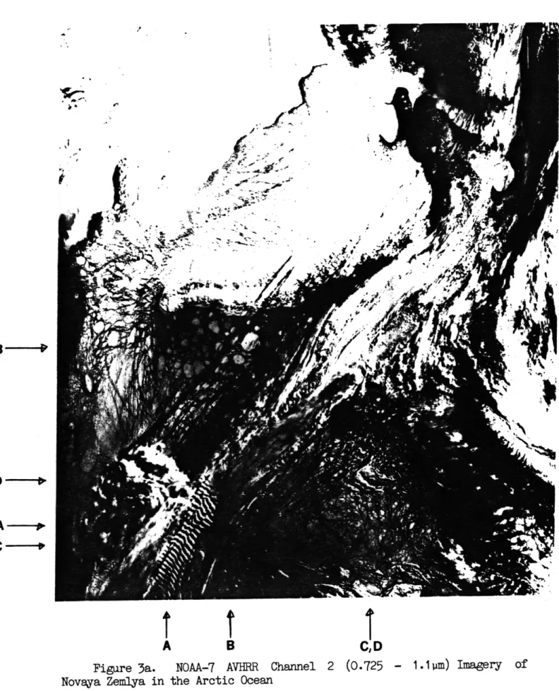
The AVHRR imagery in Figures 3a, 3b, and 3c were taken simultaneously in daylight hours over the Arctic Ocean. The Channel 2 imagery of Figure 3a is shown here instead of. the Channel 1 imagery because boundaries of water with other surfaces contrast more sharply in the Channel 2 spectral range 0.725 - 1.lim, as previously mentioned. Even though some of Channel 2 is technically outside the "visible" part of the spectrum, its charac-teristics for the most part resemble those of the Channel 1 visible band. Thus during the following discussion Channel 2 imagery may be referred to

-10--WATER

--- ICE

0.1 1.0 10.0 100.0

OPTICAL THICKNESS

Figure 2. Theoretical Calculations of the Reflectance at 3.7pm

Versus Optica1 Thickness for Plane Parallel Clouds With Various

r ,'" w . . . • 4 . . . 4-rA

:

T

B

Figure 3a. NOAA-7 AVHRR Channel 2 Novaya Zemlya in the Arctic Ocean

'A'

"i

C,D

'1

C:

_i2i.

9'

A

B

C,D

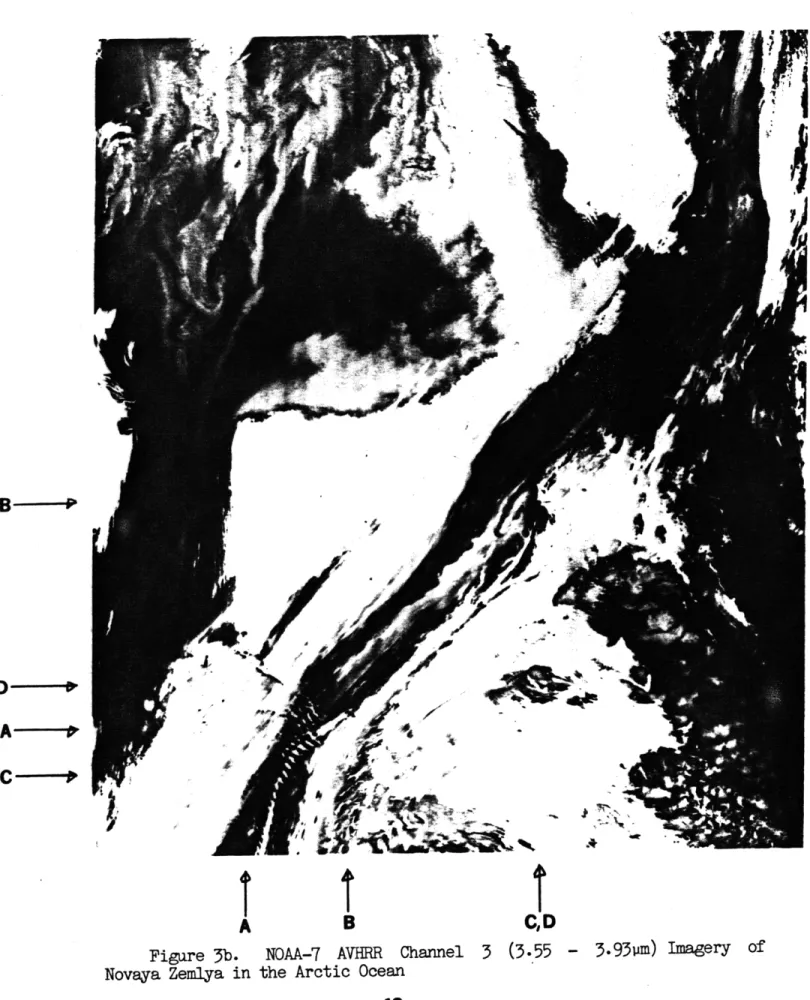
Figure 3b. NOAA-7 AVHRR Channel 3 (3.55 - 3.93pm) Imagery of Novaya Zemlya in the Arctic Ocean

-U-I

1.1

B

-D

ir~i

A B C,D

Figure 3c. Novaya Zemlya in

NOAA-7 AVHRR Channel

the Arctic Ocean

4 (10.3 - 11.3pm) Imagery

-14-B - 0

as "visible" imagery.

Bright tones in Figure 3a denote high albedos (e.g., clouds, snow/ice covered land), while darker tones denote lower albedos (e.g., ice free

surfaces, forests). Black is open ocean. The Channel 4 IR imagery is shown in Figure 3c. Cold temperatures are represented by bright tones and warm temperatures by dark. At nighttime, the tones of gray in Channel 3 imagery would exhibit the same general characteristics as the imagery of Channel 4, i.e. cold is bright and warm is dark. In daytime, reflected

incident solar radiation contaminates this scheme, as can be seen in com-paring Figure 3c with Figure 3b.

Note most obviously that the 3.7um imagery is not always dark (hot) where the 11 m imagery is dark. Likewise, the two imagery types are not always correspondingly bright (cold). At night, in the absence of any solar radiation, the 3.7 and 10.74m images would look characteristically

similar.

The point A denotes an area of high, cold (bright in the IR) cirrus clouds. Their ripples and 6hadows can be detected in the visible, and even in the IR a hint of their wavelike structure is noticeable. In the IR these clouds appear to be colder than just about any other cloud or land feature in the image, but this is not so in the near IR image 3b. In fact the point A appears considerably warmer in the near infrared image than does point B, in direct contradiction to the IR image information. As can be seen in the visible image, point B contains an area of sea ice and open ocean. The ice free ocean should be much warmer than the high

cirrus cloud tops. This opinion is substantiated by the fact that in the IR window (3c), which is not directly affected by reflected solar radiation, the cirrus tops are indeed brighter and therefore colder than

-15-both the open ocean and the sea ice areas. The reason that the near infrared image has "inverted" this scheme is because at 3.7m, liquid water and ice/snow are good absorbers of incident solar radiation. Thus the water and ice don't reflect as much 3.7um incident solar radiation back to space as the nonwater bodies around it do, in turn making it

look colder in relation to everything around it. The cirrus clouds of region A on the other hand reflect a much more significant part of inci-dent 3.7pm solar radiation back to space (note the Figure 2 reflectances for ice particle clouds), giving them warmer brightness temperatures than the truly warmer water below. It should be kept in mind that the appearance of thin cirrus clouds in nearly any spectral region is based not only on what it reflects or emits at a given wavelength, but also is further complicated by the fact that thin cirrus transmissivities are significant. In other words, some of the radiation emitted by the

sur-faces below pass directly through the thinner parts of ice clouds, chang-ing the appearances of these surfaces noticeably.'

The cloud free, snow covered area surrounding point C illustrates a similar phenomenon. The snow effectively absorbs all of the incoming 3.7pm solar radiation, so that it does not appear warm in the Channel 3 image as the.Channel 4 image shows it to be. Note also the midlevel water

droplet cloud D. It appears warmer in the 3.7um image than does the sur-face beneath it, whereas the more truly temperature-representative

10.7pm image shows the cloud to be significantly cooler than the ground below. Water droplets reflect better at 3.7um than ice crystals do (see Figure 2). The 3.7pm reflectivities of ice crystals and water droplets are an interesting property; intercomparison of a 3.7im daytime image

with a corresponding 10.7pm image helps to discriminate water clouds (and

-16-ice clouds) from from underlying snowy backgrounds. Such discriminations

on the basis of visible and thermal IR imagery alone can often be quite

difficult.

In these images there are more illustrations of the problems encount-ered when dealing with daytime Channel 3 radiance data. Separating out reflected solar from thermal emissive effects at 3.7um during daylight hours is not a trivial task. Corrections for reflected solar radiation at 3.7jm are highly variable functions of surface properties and scene solar elevation angle, and comprise a whole study in themselves. It is for this reason that this multispectral image analysis study restricts itself to the use of nighttime Channel 3 AVHRR data.

D. Infrared Atmospheric Radiation Physics

The monochromatic .upwelling thermal radiance at the top of a non-scattering, plane-parallel, 'cloud- free atmosphere, which is in local thermodynamic equilibriunt and whose source function is the Planck func-tion, may be written as a function of pressure p at the top of the atmosphere (where p=0O) in the form (Liou, 1980)

0

Y =(O) = IX(psfc) X(sfc ) + B[T(p)] dp, (1)

ap

Psfc

where 'X is the monochromatic transmission function for wavelength X and

is often called transmittance, and where BX is the Planck emission for a

blackbody of temperature T. _{The subscript sfc denotes surface values.} The transmission function 'x(p) is

X(p) = exp(-TX(p)), (2)

and the optical depth TX is defined 0

x(p)

=

{

k

-- (p')dp'},

(3)

gases g _{P a}

p

where kX is the absorption coefficient (in units of effective cross-sectional absorbing area per unit mass of absorbing gas [LM-1 ]), p and pair are the densities of the absorbing gas and the atmosphere, re-spectively, and g is the acceleration of gravity. Optical depth is never negative; since the integrand on the right side of (3) is positive defi-nite (both kX and P/Pair are nonnegative by definition), the order of in-tegration in (3) ensures T to be positive as well. Since T>O, then from

(2) it is easily seen that transmittance 7X is always within the range O< X41. The lower the transmittance, the more opaque the atmospheric path

is to radiation of wavelength X. The cleaner or more transparent an atmospheric path is for a particular wavelengths's radiation, the smaller the value of the optical depth and the larger the transmittance. Thus near the top of the atmosphere (p+O) where there exist virtually no ab-sorbing gases or aerosols, optical depth +O as well. As the path length through the atmosphere increases then so too does optical depth, in gen-eral. The less transparent (more opaque) an atmosphere becomes, the lar-ger T becomes. ,?(Psfc) = exp(-TX(Psfc)) is usually significantly less less than 1; at the top of the atmosphere, :X(p=O) = exp(-T(p=O)) =

e- 0 = 1. In short, the transmittance is a measure of the fraction of radiant emission from a body that makes it through the atmosphere and out to space.

-18-a V (P)

The quantity on the right side of equation (1) can be regarded ap

as a weighting function. It is a wavelength and pressure (height) depend-ent function which, when multiplied by the Planck emission, gives the atmospheric contribution of level z(p) to the upwelling radiance I (0). Figure 4 shows a qualitative example of what corresponding atmospheric transmittances and weighting functions look like. The peak in the weight-ing function curves indicates where within the atmosphere originate the

most significant contributions to measured upwelling radiance. It can be shown that the levels of these peaks are given by

Zpeak = HanTx,sfc,

where TX ,sfc is the cloud free atmospheric optical depth from space to

ground level, and where H is the scale height of the particular band ab-sorber (Prinn, course notes).- This peak lies at the level z where optical depth Trx(z) from the top of the atmosphere' to z is approximately unity. Hence in window regions such' as those of the NOAA-7 AVHRR where optical

depth is small (i.e., <1 ), weighting functions attain their largest values

at the surface. On the other hand, in spectral regions where optical depth is significantly larger (i.e., >1; large optical depths are due to absorp-tion by such gases as water vapor, ozone, and carbon dioxode), then the

corresponding weighting functions peak at levels Zpeak above the surface. Observations of radiation measured within absorption bands generally only

see through the top down to middle layers of the atmosphere, since absorb-ing gases block out any radiation at their absorption band wavelengths that originates from levels below those where the gases begin to effectively absorb. Figure 4 shows weighting functions for two absorption bands with peaks at 50 mb and 400 mb, and also shows a weighting function for a "dirty" window which peaks at the surface. In summary, the quicker

5o0 100 200 400 500

85o

SWeij h1T3

Funcho(*

Trqns mi4ttace

Figure 4. Qualitative Example of Transmittances and Corresponding

Weighting Functions (after Liou, 1980)

U,

with height the transmittance for a particular wavelength approaches unity, the further through the atmosphere a satellite sensor responsive

to energy at that wavelength can see.

The term IX(Psfc) in equation (1), represents emitted surface

ra-diance, and is given by

IX(sfc) = EXBA(Tsfc), (4)

where EX is the emissivity of the emitting surface. Emnissivity is the relative emissive power of a radiating surface expressed as a fraction of the emissive power of a blackbody radiator at the same temperature. Emis-sivity is a function of both wavelength and surface (e.g., rocks, trees, ice crystals, water droplets).

Equation (4) implies that there is no incident solar radiation of wavelength X reflected back out to the atmosphere by the surface, and

likewise that there is no downward-reflected atmospheric contribution of radiation at' wavelength X which might be reflected back out by the sur-face. Also, (4) is valid for surfaces with zero reflectivities at

wave-length X. In any event, (4) is certainly valid for the AVHRR window

re-gions at night, when incident solar fluxes which might affect Channel 3

are nonexistent.

Substituting the form (4) for IX(Psfc) into (1), the following

ex-pression for IX(O) is obtained:

0

IX(O) = eXBX(Tsfc) (Psfc) +J BX[T(p)] ap, p. (5)

ap

Psfc

Equation (5) gives a form in pressure coordinates for the upwelling

ther-mal radiance at a single (monochromatic) wavelength. However, space-borne satellite sensors are designed to measure radiant energies within

some wavelength range (X1,X 2). The observed upward spectral radiance

Iobs sensed by a downward pointing radiometer in band width (X1,X2) (call

this band width Channel j, say) is a weighted average of the monochromatic

radiances IX(O) (from (5)), and is given by

SIx(O)Rj(X)dX

0

o

2bs,j(0 ) = , (6)

0

where Rj(x) is the response function for channel j, and X is the central wavelength in the band width (X1,2). 7 is a functionXj of channel j.

The response function Rj(X) takes on values between 0 and 1, and is often expressed in percent. Rj(X) is a measure of Channel j's sensor response to radiation at wavelength k; if Rj(X) is 1, the sensor detects 100% of the energy radiated at wavelength X, whereas if.Rj(X) is .89, then the sensor only detects 89% of the total energy radiated at wavelength X. Sensors are designed to have response functions Rj(X) that are zero outside some wavelength range (X1,X 2); within this range it is generally

a rapidly varying function of wavelength. Response functions are usually depicted in graphical or tabular form. They are predetermined by the

instrument manufacturer according to customer needs and the properties of the sensor optical components. The response functions for the five

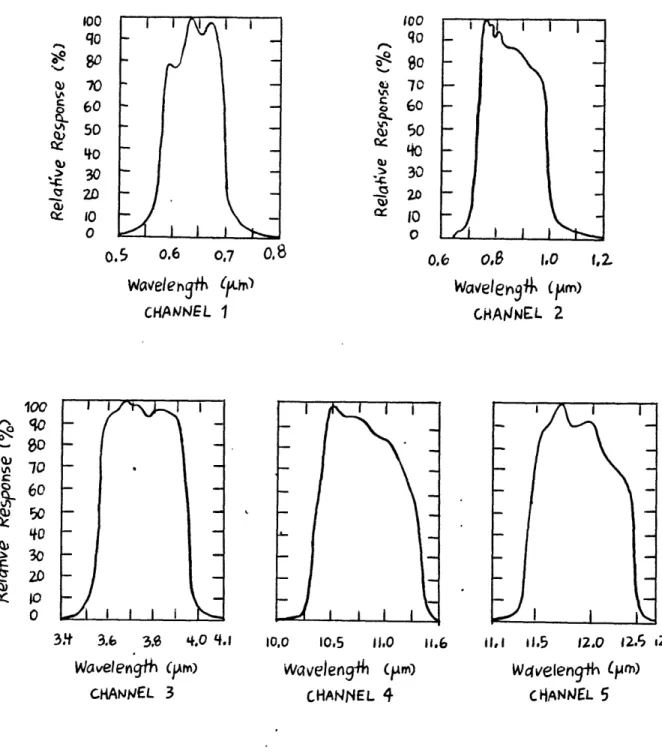
NOAA-7 AVHRR Channels 1, 2, 3, 4, and 5 are shown in Figure 5.

The spectral radiance Iobs(O) measured by a satellite sensor is given

x

by equation (6), with IX(0) as given by equation (5). The Planck radiance B (T) is

100 0 80-0 70 S60 S50

30

I.-60

Figure 5. _{Response Functions for the NOAA-7 AVHRR Window Channels} 1-5 (from Kidwell, 1983)

2hc2 1

BX(T) = 1 (7)

B5 exp(hc/AkT)-l' (7)

where h = 6.63 x 10-27 erg sec photon-1 is Planck's constant,

c = 3 x 1010 cm sec-1 is the speed of light, and k = 1.38 x 10-16 erg oK-1 molecule-1 is Boltzmann's constant. The brightness temperature, or equiv-alent blackbody temperature, is defined as

he 1

Tr = (8)

Br Ak In(2hc/A s BA+1)'

(8)

and corresponds to the temperature a blackbody would have if it emits radiation at an intensity BX(TBr). When satellite-measured radiances are

inverted to obtain brightness temperatures using I°bs in place of BX

in equation (8), for most objects the temperatures TBr thus obtained are not true thermodynamic temperatures. They are generally lower than actual, due 'primarily to atmospheric attenuation effects and surface emissivity properties.

Substituting the form (5) for IX(O) into (6) yields

Ibs,j(₀o) = B(Tsfc) ofX(Pf c) Rj (X)dX O 0 0 + X[T(p)] p R i)dX (6b) Psfc

Since the response function Rj(X) is identically zero outside some

spec-W xj,z

tral interval Xj,l(<Xj,2, then note that the fdX + fdX in equation (6)

O Xj,

0 X<xj,1 or X>Xj,₂ Rj(X) =

<1 Xj,1l"Xxj,2. The above equation for IobS(o) can then be written

Iobs,j(0) =

xBTf

Rj (X)dX -Xj Psfc

ji

+

[ T()l1 pdR (;

jRj(A)W d ii

S

)dal

Now if the spectral region X1<X<X is sufficiently small that BX(T) varies slowly with wavelength Xe[X1,X2], then BX may be replaced with Bj(T) to

a good approximation (in other words, the variation with wavelength of BX is small and smooth over the interval Xi XZ and hence BX can be

effective-ly removed from inside the fdA in the first term on the right side of

equation (9)). Assuming similarly that EXBX(Tsfc) + Ej j(Tsfc) (for most

earth surfaces, EX is relatively independent of X over the range of an AVHRR channel (Dozier, 1981)), then equation (9) can be written

Sobs'(0) EjBj'(Tsfc)

l

(psf)Rj(A)dA

where the overbar ""' is defined as some average wavelength operator over the interval Xj,1XXj,z. Now consider the double integral term

ffdpdX

Aj,2 o Aj,1.

dp

R;

Aj,1

Pi

Psfc

j,'

Again invoking the assumption that the variation of BX(T) with respect to wavelength X is small and smooth over the interval Xj41( , the above be-comes

0

0

j,2

- Rjj(dA dp

Psf C _A

Substitution of the above form for the

ffdpdX

obsj I

1

A A-2

j,z

:ABjd

C

(o)p

(

AP.Rcad

SRj

(~a

A

o _Aj,

(

+

f

j[Tp)J

aI(p)

Rj(A) ddp

i

(11)

Psfc

Aj,1

Defining the spectral transmittance a-(p) as

(p) Al (12a)

f Rj(A)dA

,-26-a

CT.

(P)

and the spectral weighting function as

f

a

R(ap

)

_J:,.:) ap

(12b)

ap Aj,2

then (11) can be written in the simpler form

0

bs(0) j(Tsfc) Psf) + Bj [T(p)] p. (13)

h 'ap

Psfc

Both the spectral transmittance (12a) and the spectral weighting function (12b) take into account the sensor response function Rj (X). Note the similarity of the form of, equation (13) to that of equation (5).

Equation (13) gives the form for satellite-observed radiances. How-ever, keep in mind that the -form (13) for Ibs(O) is an approximation to the exact form (6) for two reasons. First of all the Planck emittance BX(T), along with the surface emission EXBk(Tsfc), was considered essen-tially independent of wavelength for a given spectral region l <<2', as previously stated. This is not a bad assumption at all for "small" spec-tral intervals, but the NOAA-7 AVHRR spectral intervals are not so small as to constrain BX(T) to be precisely constant within them. For typical terrestrial temperatures, the approximation BX(T) + Bj(T) (remember that even the average Bj is still a function of X (i.e., a function of Channel number)) is better for the longer IR wavelength AVHRR channels than it

is for the shorter ones, as is depicted in Table 2. Variations of black-body radiances for the 3.7im Channel 3 sensor are on the order of one order of magnitude, whereas they are more consistent for the wavelengths

Lower bound of R.(X) (in m) 3.442 10.0 11.1 BX (273 ₂oK) (Watts m- 2 Pm-1 ster-1 ) .055236 6.156901 6.181713 Upper bound of R.(X) (in im) 4.142 11.65 12.8 B (273 oK) (Watts m-2 um-1 ster- 1 ) .291088 6.086909 5.739613 Table 2. Values of Planck blackbody radiances at 273 oK for the

lower and upper wavelength bounds of the response func-tions for NOAA-7 AVHRR Channels 3, 4, and 5

-28-Channel 3

Channel 4 Channel 5

in the Channel 4 and 5 regions. In addition, it must be remembered that the response functions R for each of the three channels listed in Table 2 are small for some of the wavelengths for which they are defined. In light of these consequences, the choice of the definition for Bj(T) should be made with care and caution, especially when using (13) to theoretically estimate upwelling thermal radiances observed by the AVHRR Channel 3 sensor.

Second, the emissivities E. were also considered independent of X

for X1 <X 2. However, the assumption EX + Ejturns out to be far better

than the assumption BX + Bj, since emissivities don't change much over spectral intervals like those of the AVHRR. It is far more a problem to be able to accurately specify the emissivities eX as a function of varying

surface types such as vegetation, forests, snow, and water.

The form (13) for I2bs(0) is more desirable than the form (6b) as far

as numerical integration techniques are concerned. Equation (6b) contains a double integral term fjdpdx + EEApmAXn, whereas equation (13) contains

Xp n m

at most a single integration

fdp

reduc-m

tion in computational iterations offered by (13) is gained at the expense

of the two approximations BX(T) B-j(T) and exBX(Tsfc) + ejBj(Tsfc) and the subsequent associated reductions in the accuracy of the computed

E. Cloud Property Retrieval Method

Equation (13) for the satellite-observed radiances can be written in pressure coordinates (at the top of the atmosphere, p=O):

0

(

0) E E f'Bj

(Ps(r

+3

dp,

P Psf

in height coordinates (at the top of the atmosphere, z=--):

00

I

+

dE

Z=0

or in transmission coordinates (at the top of the atmosphere, X=1

obs,j T( X

Ib () Cj j (T+,S ₎ V jsif + T( .r ] d " (13c)

Each of the three equations (13a) - (13c) yield exactly the same radiances for the continuous vertical grid case. However when they are approximated in quadrature form, different I2bs values may be obtained for each of the three vertical coordinate systems. The following.example illustrates this point.

Recall that the form (2) for the transmission, which shows the trans-mission function to be logarithmic in nature. Recall, too, that for atmo-spheric windows the transmission function takes on its lowest values at the surface and monotonically increases upward with height. With these facts

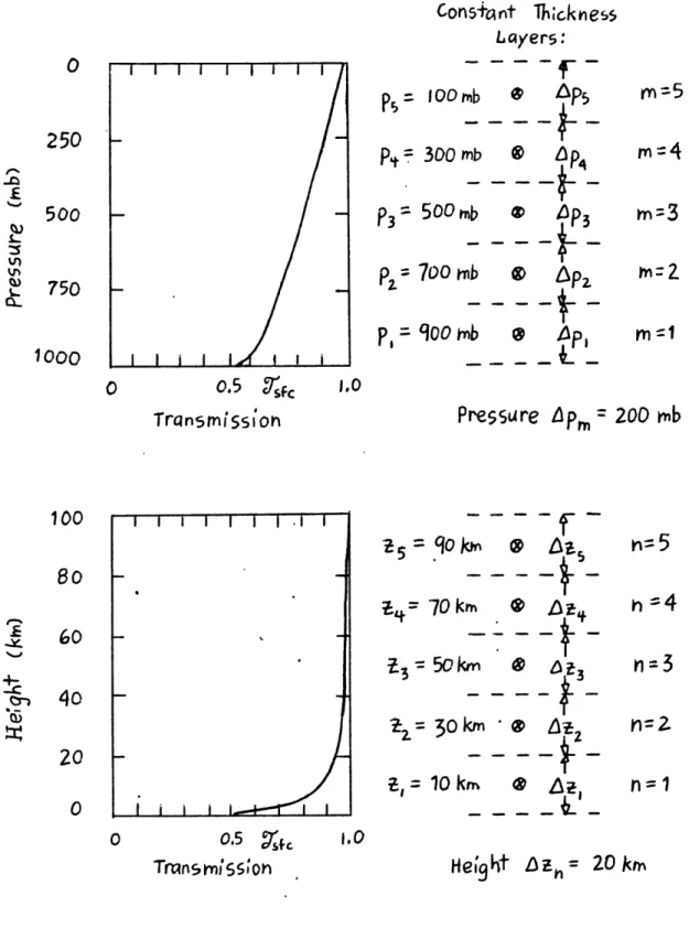
in mind, consider now the qualitative plots of a window transmission func-tion versus two of the three aforemenfunc-tioned vertical coordinates, namely pressure and height, as drawn in Figure 6.

Assume a simple five layer quadrature for the equations (13a) and

-30-0

250

750

----

Lps

P3

Soo0b

a P3_

----2-Pt

700

enb

p2

-,

= 900

-

4b

p,-p

=qoo00 nb

1?PI

=3

m2

Pressure

p,

₂₀₀

_rnb

---

-f--m

krn

Figure 6. A Qualitative Plot of the Transmission Function for a

Typical Window Region, Graphed Versus Pressure and Height as Vertical Coordinates 100 I-' .-t ki3 60

40

20

Eq= 70 k

3

= 50

k

Ii=

301

t,

= 10 k

5

n=

3

n=

1

(13b), respectively, as follows:

S(o)

ej

where Pm - is the pressure coordinate weighting function, and

ap p_Pr

obs,j ---- 5

I 3 (o') Ej0j(Tsf) (0) +

Bj

n=1

where Zn is the height coordinate weighting function. For the

above hypothetical case, the layer thicknesses Apm for the pressure

coord-inate quadrature are given by

Ap_ - _Ps -O 200 mb,

and the layer centers pm are 900, 700, 500, 300, and 100 mb. The layer

thicknesses Azn for the height coordinate quadrature are given by

'100 km - O km

- m 20 kin,

h,

5

and the layer centers zn are 10, 30, 50, 70, and.90 km. In the altitude case note that at least 4 out of 5 of the layer centers lie in atmo-spheric regions where the transmissions are quite close to one. The

atmospheric contribution to upwelling thermal radiance is very small in

these regions, i.e., is very small from levels with transmittances close to 1, since temperatures are quite cold and absorption by constituents

in atmospheric window regions is small. Hence, 4 out of the 5 quadrature points in the vertical grid for equation (14b) add essentially no contri-bution to Iobs.

Clearly the bulk of the atmospheric window contribution to Ibs comes from

-32-the lowest atmospheric levels where tropospheric window absorber concen-trations (mainly water vapor) are highest and temperatures are usually warmest. The pressure coordinates (equation (14a)) are clearly superior to the altitude coordinates but still they are not optimal. Indeed, un-like the layers depicted in Figure 6, it would be advantageous to choose a radiance quadrature scheme the majority of whose layers' centers lie at levels much closer to the ground. Choosing layers of equal transmit-tance thickness alleviates this finite layer quadrature problem in the best possible way.

The five layer equal transmittance quadrature for (13c) can be writ-ten

ObSJ) 5

okj , 5 T

- (. ) - ) s.+ +j.(Tsf TS) 4" j , (14c)

where the constant layer thickness A t~j1 is given by

3 5

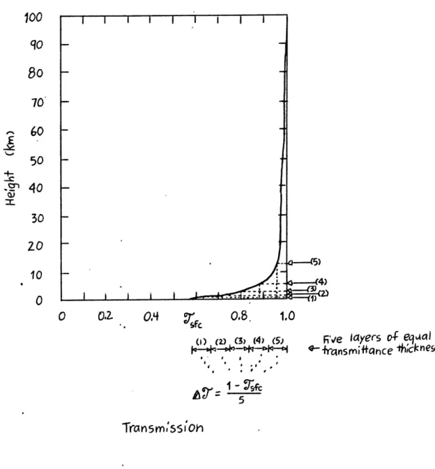
Figure 7 depicts the five layers of equal transmittance computed in the above fashion. The majority of the layers lie close to ground level where most of. atmospheric contributions to upwelling thermal radiance originate. Note that the centers of the first four layers of equal transmittance lie below the. center of the first equal height layer. Clearly, then, the transmittance method (14c) is the proper, most desir-able coordinate system to use in order to obtain the most accurate quad-rature possible for equation (13).

The satellite-observed radiance model used in this study is therefore expressed in transmission coordinates. In summary, for the continuous

-33-O, C 0.8. (I) (2) (3) (4) (5

~qDQ-DPG

5. I

5 .

Fi'Ve layers of eAal 4-fransmi4+nce ;~hckneS

TrnSm;551'Oh

Figure 7. A Qualitative Plot of the Transmission Function as in Figure 6, But Depicting the Heights of the Centers of the Five Equal Transmittance Thickness Layers. Locations of the Centers of These Layers are Denoted by Arrows

-34-100

qo

60

50

40

20o

0

case it is

I

s ( )" Bj Tj Aj (15a)

In quadrature form, (15a) can be written

I

where Ibs, j (1) is the theoretically expected satellite observed ra-diance, j is the NOAA-7 AVHRR channel number (j=3,4,5),-cj is the sur-face emissivity valid over the spectral interval of Channel j, Fj(T) is the average value of the Planck radiance valid over the spectral in-terval of Channel j, 9- j is the spectral transmittance (as defined by

(12a), a is the layer counter, L is the number of layers to be used in the quadrature, and where each layer's thickness A ,j is given by

1 -

_j,

c

1 5fe

(15c)

3j

L

Note from the above equation (15c) that the "dirtier" the window (i.e., the smaller the 7sfc), the thicker the layer (the larger the AT) in altitude.

The upwelling thermal radiance measured by a satellite sensor for AVHRR Channel j is given by the equations (15). Now consider a mixed scene composed of a cloud of temperature Tcld, occupying a portion p of a sen-sor's field of view, along with the surface at temperature Tsfc, occupying the portion p-1 of the sensor field of view. Then the upwelling radiance Isat,j (=1) sensed by Channel j at the top of the atmosphere will be a linear combination of the integrated radiances Icld,j(1) (emitted by a

-35-total cloud cover) and Iclr,j (1 ) (emitted through a completely clear

atmo-sphere), and is given by

Isat,j(i) = (p-1)Iclr,j(1) + Icld,j(1), (16)

where p is the amount of cloud cover (O<p1), and where Lglr,j(1) and ICld,j(1) are computed using equations (15) with Ej Tsfc, and Isfc equated with the emissivity, temperature, and transmission for the ground and cloud top, respectively.

It is important to note that the cloud contribution Icld,j to the satellite-observed radiance Isatj is computed assuming that clouds act as an emitting surface through which no radiation can pass. In other words, in order for (16) to be valid the optical depths t (see equation

(3)) of the clouds being sensed must be significantly greater than unity so that no radiation emitted by levels .underlying the clouds passes

through those clouds. The cloud transmissivity must be low (no greater, say, than 0.1). Transmissivity is defined as follows.

On the basis of conservation of energy, the following relation for the

transfer of radiation through a scattering and absorbing medium must hold

(Liou, 1980):

tX + rX + eX = 1,

where tX is the transmissivity, rx is the reflectivity, and ex is the emissivity. The transmissivity is defined as the ratio of the outgoing radiation to incoming radiation. Reflectivity is defined as the ratio of the reflected (backscattered) intensity to the incident intensity.

Emis-sivity is as defined in equation (4). Note that transmissivity, reflect-ivity, and emissivity are each a function of wavelength, and that the range of values each can take on is in the interval [0,1].

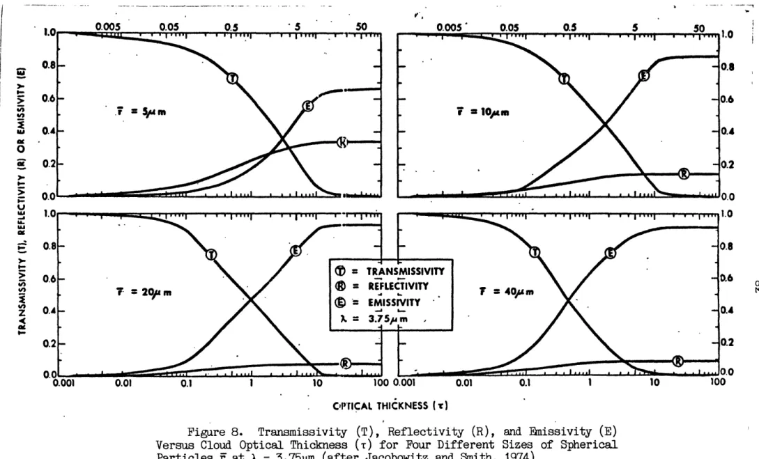
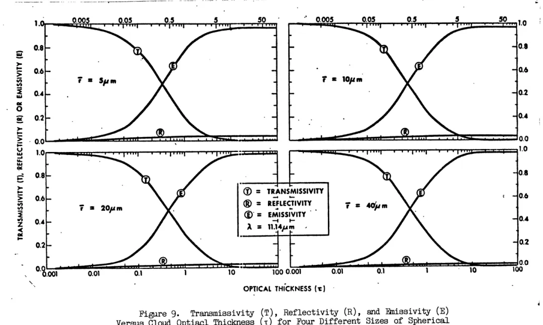
-36-Figures 8 and 9 contain transmissivity, emissivity, and reflectivity

plots for various average cloud droplet sizes Fand cloud optical depths T, at X=3.75 and 11.14om, respectively. Table 3 lists the total cloud

opti-cal depths which correspond to cloud transmissivities equal to 0.1, as re-trieved from the graphs in Figures 8 and 9. For a given cloud drop size r, note that optical depths are generally lower in the Channel 4 and 5

spec-tral regions than they are in the Channel 3 specspec-tral region. This is equivalent to stating that the attenuation (absorption plus scattering) of 3.7um radiation by water droplet clouds is smaller than it is for

ra-diation at 11um.

Hence to have transmissivities that are low enough (<0.1) for the

Ic1d,j(I) term of equation (16) to be adequately described by equation

A

(15) requires that clouds within the sensor field of view have optical depths no smaller than those values listed. in Table 3. This requirement

restricts the successful use-of equation (16) for Isat,j to fields of view_A

within which only lower clouds exist. Low clouds are generally water

drop-let clouds; the lower they are the warmer their environment is, and hence

the larger the cloud droplets will tend to be (except for ground fog, which nearly always consists of tiny water droplets). Therefore in addition to only being able to use 3.7pm Channel 3 nighttime imagery, this cloud

Droplet Wavelength

Size X = 3.75om X = 11.14um

' = 5pm 9 2

S= 10m 8 3

F = 20Pm 7 3

f = 40Pm 3 3

Table 3. List of optical depths t where cloud transmissivities

TX equal 0.1, for various spherical particle sizes F and

0.005 0.05 0.5 5 50 0.005 0.05 0.5 5 50 1. a I I w 4 1 1 1 1 1 w I I I I I o I I I .0 0.8 - - o. 5 0.6 - - -0.6 S10 _m 0.4 - - -0. 0.- -0. TRANSMISSIVITY 0.2 -0o 0.001 0.01 0.1 10 100 0.001 0.01 0.1 10100 C'PTICAL THICKNESS (r)

Figure 8. Transmissivity (T), Reflectivity (R), and Emissivity (E)

Versus Cloud Optical Thickness (r) for Four Different Sizes of Spherical

-4 0..5 5 50 0.005 0.05 0.5 5 50 1.0 0.8 - - -0.8 0.6- -1 - 0.6 . SP m = 1014 m s 0.4- -0.2 0 0 0.2- -- 0.4 1.0 " 1.0 Ui 08 _-0.8 0.8-TRANSMISSIVITY 0.6 - - 0.6 c > 0.2 _{(ID REFLECTIVITY} 0 4 M 4 21 m .4 20" I . = EMISSIVITY 0.4 00- 0.4 Z _A11.14 0.2 -0.2 " I ") Tn"--0.0 0- .001 0.01 0.1 1 10 100 0.001 0.01 0.1 1 10 l00 OPTICAL THICKNESS (C)

Figure 9. Transmissivity (T), Reflectivity (R), and Emissivity (E)

Versus Cloud Optiacl Thickness (T) for Four Different Sizes of Spherical Particles F at X = 11.14pm (after Jacobowitz and Smith, 1974)

analysis study also must restrict itself to the specification of cloud

parameters for lower, relatively thick water phase clouds. Higher clouds,

in addition to being made up of smaller water droplets (which would sub-sequently require them to be of greater vertical extent to acquire the

necessary optical depths), might also be composed of ice phase particles.

Ice crystal attenuation properties differ significantly from those of

spherical water droplets, and many types of ice clouds encountered in the atmosphere (e.g., cirrus) generally have much higher transmissivities

than even the thinnest of water droplet clouds. The problem with optic-ally thin clouds lies in the fact that significant amounts of radiation emitted from lower layers beneath the cloud pass through it and

subse-quently reach the satellite radiometer. A more complicated radiance

model would have to be developed to account for such effects; however, keep in mind that even for high, optically thin clouds,

satellite-observed brihitness temperatures are typically low enough to allow for

their straightforward detection.

A computer code was written to compute a series of Igat,j(1)'s using (16) and a 15-layer model (L=15 in (15)), for a number of different atmo-spheres. These computations were functions of temperature profile, transmission'profile (which itself is dependent on satellite seeing angle), and the amount of cloud cover p. A hypothetical sample set of

such Isat,j(1) calculations -for each of the NOAA-7 AVHRR Channel 3, 4,

and 5 radiometers is shown in Tables 4-7.

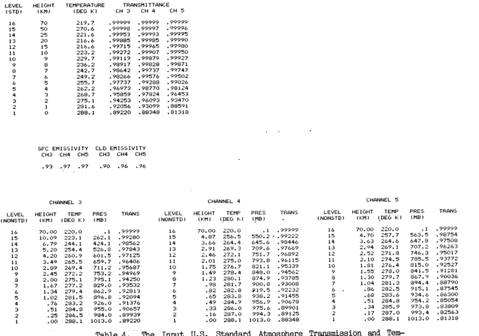
The top part of Table 4 contains the input U.S. Standard Atmosphere transmittances Y , j for each of the three AVHRR channels indicated, along with the input temperature profile. The transmittances were calculated using AFGL's computer code RSAT (personal communication, Dr. Robert A.

LEVEL (STD) 16 15 14 13 12 11 10 9 8 7 6 5 4 3 2 1 SFC EMISSIVITY CH3 CH4 CH5 .93 .97 .97 CHANNEL 3 TRANSMITTANCE CH 3 CH 4 CH 5 HEIGHT TEMPERATURE (KM) (DEG K) 70 219.7 50 270.6 25 221.6 20 216.6 15 216.6 10 223.2 9 229.7 8 236.2 7 242.7 6 249.2 5 255.7 4 262.2 3 268.7 2 275.1 1 281.6 0 288.1 .99999 .99998 .99953 .99885 .99715 .99272 .99119 .98917 .98642 .98266 .97737 .96973 .95859 .94253 .92056 .89220 .9999 .99997 .99993 .99985 .99965 .99907 .99879 .99828 .99737 .99576 .'99288 .98770 .97824 .96093 .93099 .88348 CLD EMISSIVITY CH3 CH4 CH5 .90 .96 .96

LEVEL HEIGHT TEMP (NONSTD) (KM) (DEG K) 70. 00 10.09 6.79 5.20 4.20 3.49 2.89 2.45 2.00 1.67 1.34 1.02 .76 .51 .25 .00 220.0 223. 1 244.1 254.4 260.9 265.5 269.4 272.2 275.1 277.2 279.4 281.5 283.2 284.8 286.5 288.1 PRES (MB) .1 262.1 424.1 526.8 601.5 659.7 711.2 753.2 795.1 829. 0 862.9 896.8 926.0 955.0 984.0 1013.0

TRANS LEVEL HEIGHT TEMP (NONSTD) (KM) (DEG K) .99999 .99280 .98562 .97843 .97125 .96406 .95687 .94969 .94250 .93532 .92813 .92094 .91376 .90657 .89939 .89220 70.00 4.87 3.66 2.91 2.46 2. 01 1.75 1.49 1.23 .98 .82 .65 .49 .33 .16 .00 220.0 256.5 264.4 269. -272.1 275. 0 276.7 278.4 280.1 281.7 282. 8 283.8 284.9 286.0 287.0 288.1 PRES (MB) .1 550.2 645.6 709.6 751.7 793.8 821.1 848.0 874.9 900.8 919.5 938.2 956.9 975.6 994.3 1013.0 TRANS .9999 -. 99222 .98446 .97669 .96892 .96115 .95339 .94562 .93785 .93008 .922.32 .91455 .90678 .89901 .89125 .88348

LEVEL HEIGHT TEMP (NONSTD) (KM) (DEG K) 70.00 4.70 3.63 2.94 2.52 2.10 1.81 1.55 1.30 1.04 .86 .68 .51 .34 .17 .00 220,. 0 257.7 264.6 269.1 271.8 274.5 276.4 278. 0 279.7 281.3 282.5 283.6 284.8 285.9 287.0 288.1

Table 4. The Input U.S. Standard Atmosphere Transmission and

Tem-perature Profile (Top), Ground and Cloud Emissivities (Middle), and

the Vertical Grid Levels for the 15 Iayer Equal Transmittance Radiance

Model Calculations (Bottom)

.99999 .99996 .99995 .99990 .99980 .99950 .99927 .99871 .99747 .99502 .99026 .98124 .96453 .93470 .88591 .81318 CHANNEL 4 CHANNEL 5 PRES (MB) .1 563.5 647.8 707.2 746.3 785.5 815. 0 841.5 867.9 894.4 915.1 934.6 954.2 973.8 993.4 1013.0 TRANS .99999 .98754 .97508 .96263 .95017 .93772 .92527 .91281 .90036 .88790 .87545 .86300 .85054 .83809 .82563 .81318

McClatchey). This code is designed to compute atmospheric spectral

trans-mittance functions (as defined by equation (12a)), and takes into account absorption by well-mixed gases, water vapor, the effects of varying

atmo-spheric temperature, and the effect of. varying satellite viewing angle (which determines optical path length). Tables of the spectral trans-mittance functions for each of the AVHRR window Channels 3, 4, and 5

are listed in Appendix A as a function of atmosphere (e.g., Arctic, U.S.

Standard, and Tropical) and satellite viewing angle.

In the middle of Table 4 are listed the cloud and surface emissivi-ties that went into the 15-layer radiative transfer model. A list of

emissivities as a function of wavelength for the clouds and surfaces encountered in this study can be found in Appendix B.

Finally, at the bottom of Table 4 are listed the levels bounding the

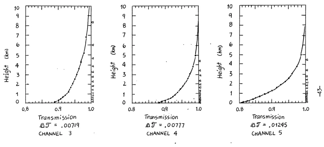
15 layers of equal transmittance thickness, along with their corre-sponding temperatures, for each of the AVHRR Channels 3, 4, and 5. Ob-serve that nearly all the layers of the transmittance coordinate grid lie in the lowest 5 km or so of the atmosphere (recall the previous ar-guments leading up to Figure 7), as is well illustrated in Figure 10. The transmittances listed in Table 4 were computed for U.S. Standard at-mospheric temperature and aerosol profiles, and also for a vertical path from the ground to space (i.e., the satellite viewing angle is zero). Note that the A 9' for Channel 5 is the largest of all three channels; this is due to the fact that Channel 5 is the dirtiest of the 3 infrared AVHRR windows. With surface/cloud emissivities and atmospheric

trans-mittances and temperatures entered in, the radiance code then computes estimates of satellite-measured upwelling thermal radiances as defined

by equation (16).

-42-(0

5

44

/L-

,oo71q

Trans mi55 ion

/r = ,00777 CHANNEL 4 1,0 0.S Trans m iss55'o n

/L6

=

.01245

Figure 10. Plots of Transmittance for Each of the NOAA-7 AVHRR Channels as a Function of Altitude for the U.S. Standard Atmosphere

Example of Table 4. The Arrowheads at the Right Side of Each of the

Three Plots Indicate the Position of the Centers of Layers of Equal Transmittance Thickness

--I

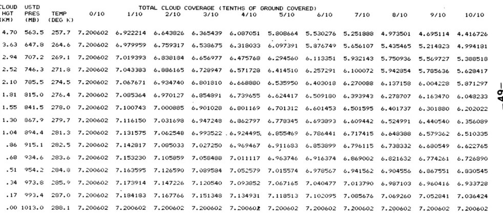
Tables 5a and 5b list the results of Channel 3 radiance computations

Isat,j(1) for the temperature, transmittance profile of Table 4 and Fig-ure 10, and for various cloud top heights and fractional cloud covers.

Fractional cloud cover runs along the top of each Table, and varies from 0 (clear) to 10/10's (completely cloudy) coverage in steps of 1/10. Along the side of each of the Tables is listed the height and temperature of the cloud top (in km and OK, respectively), just next to a list of

pres-sures which correspond to the indicated heights and temperatures. (The

pressures are just reasonable estimates of actual case pressure values,

and are listed for reference purposes only.) To find the upwelling

ther-mal radiance measured by the Channel 3 sensor whose field of view con-tains a cloud covering 80% of the underlying ground, and whose top

tem-perature is 277.2 oK, slide across the top of Table 5a to the 8/10 column

and down the Table to the 277.2 OK (1.67 km) row to read off a thermal radiance valdAe of .169036 Watts m- 2 p1rl ster-1. A simple linear inter-polation can be used to, determine thermal radiance values for clouds whose fractional coverage and/or top temperatures lie between the values

listed in the Tables.

Tables 5a and 5b contain essentially the same information; they

dif-fer only in the atmospheric vertical extent of their tabulations (note

the differences in the heights of the cloud top levels listed down the

left side of the Tables). Table 5a contains radiances for cloud tops at each of the lowest 15 levels which bound the layers of equal transmit-tance thickness, while Table 5b lists radiances for cloud tops at the lowest 10 km of the atmosphere in increments of 1 km. Table 5b was

de-rived from Table 5a using a simple linear interpolation scheme.

SATELLITE-OBSERVED THERMAL RADIANCE FOR NOAA-7 AVHRR CHANNEL 3, IN WATTS/M2-MICRON-STER

TOTAL CLOUD COVERAGE (TENTHS OF GROUND COVERED)

.227054 .228869 .230936 .232920 .234737 .236588 .238169 .239880 .241336 .242917 .244632 .246081 .247597 .249202 .251665 .202444 .206074 .210207 .214175 .217809 .221511 .224674 .228095 .231008 .234170 .237599 .240498 .243528 .246739 .251665 2/10 3/10 4/10 .177833 .183279 .18478 .195430 .200881 .206434 .211179 .216311 .220679 .225423 .230566 .23491"4 .239460 .244276 .251665 .153223 .160483 .168749 .176685 .183953 .191357 .197684 .204526 .210351 .216675 .223533 .229331 .235392 .241814 .251665 5/10 .128613 .137688 .148020 .157940 .167025 .1762:30 .184188 .192741 .200022 .207928 .216500 .223747 .231324 .239351 .251665 6/10 .104002 .114892 .127291 .1391196 .150097 .161203 .170693 .18057 .189693 .199180 .209468 .218164 .227255 .236888 .251665 7/10 .079392 .092097 .106562 .120451 .133169 .146126 .157198 .169172 .179365 .190433 .202435 .212580 .223187 .234425 .251665 8/10 .054781 .069301 .085833 .101706 .116242 .131049 .143702 .157387 .169036 .181606 .195402 .206997 .219119 .231962 .251665 9/10 10/10 .030171 .046506 .065104 .082':61 .09Q314 .115972 .130207 .145602 .158708 .172938 .188369 .201413 .215051 .229500 .251665 .005560 .023710 .044375 .064216 .082386 .100895 .116712 .133818 .148379 .164191 .181336 .195830 .210982 .227037 .251665

Channel 3 Radiance Computations

Cloud Covers and Cloud Top Heights. _{The Heights are the Levels}

Bound-ing the Lowest 15 _{Equal-Transmittance Layers} 1/1 CLOUD HGT (VM) 10.09 6.79 5.20 4.20 3.49 2.89 2.45 2.00 1.67 1. 34 1.02 .76 .51 .25 .00 USTE PRES (MB) 262.1 424. 1 526.8 601.5 659.7 711.2 753.2 795.1 82g.0 862.9 896.8 926.0 955.0 984.0 1013.0 TEMP (DEG K) 223.1 244.1 254.4 260.9 265.5 269.4 272.2 275. 1 277.2 279.4 281.5 283.2 284.8 286.5 288. 1 0/10 .251665 .251665 .251665 .251665 .251665 .251665 .251665 .251665 .251665 .251665 .251665 .251665 .251665 .251665 .251665

SATELLITE-OBSERVED THERMAL RADIANCE FOR NOAA-7 AVHRR CHANNEL 3, IN WATTS/M2-MICRON-STER

TOTAL CLOUD COVERAGE (TENTHS OF GROUND COVEREL)

8/10 .055198 .059587 .063977 .068366 .077503 .089013 .105783 .128403 .157348 .196189 .251665 9/10 10/10 .030640 .006081 .035578 .011568 .040516 .017055 .045453 .022541 .055733 .033962 .068681 .048349 .087548 .069313 .112995 .097587 .145558 .133769 .189255 .182320 .251665 .251665

Channel 3 Radiance Computations for Various

Cloud Covers and Cloud Top Heights. _{The Heights Range From} 0 to 10 km in Increments of 1 km 1/10 2/10 CLOUD HOT (1KM) 10 9 8 7 6 5 4 3 1 0 USTD PRES (MB) 265.0 308.0 356.5 411.1 472.2 540.5 616.6 701.2 795.0 898.6 1013.0 TEMP (DEO K) 223.2 229.7 236.2 242.7 249.2 255.7 262.2 268.7 275.1 281.6 288.1 0/10 .251665 .251665 .251665 .251665 .251665 .251665 .251665 .251665 .251665 .251665 .251665 .227106 .227655 .228204 .228752 .229895 .231333 .233430 .236257 .239875 .244730 .251665 .202548 .203645 .204743 .205840 .208124 .211002 .215194 .220849 .228086 .237796 .251665 3/10 .177990 .179636 .181282 .182928 .186354 .190670 .196959 .205441 .216296 .230861 .251665 4/10 .153431 .155626 .157821 .160015 .164584 .170339 .178724 S190034 .204506 .223927 .251665 5/10 .128873 .131616 .134360 .137103 .142814 .150007 .160489 .174626 .192717 .216992 .251665 6/10 .104315 .107607 .110899 .114191 .121043 .129676 .142254 .159218 .180927 .210058:3 .251665 7/10 .079756 .083597 .087438 .091278 .099273 .109344 .124018 .143810 .169138 .203123 .251665 Table 5b. Fractional