Classical capacity of the free-space quantum-optical channel

Classical Capacity of the Free-Space

Quantum-Optical Channel

by

Saikat Guha

Bachelor of Technology in Electrical Engineering,

Indian Institute of Technology Kanpur (2002)

Submitted to the Department of Electrical Engineering and Computer

Science

in partial fulfillment of the requirements for the degree of

Master of Science in Electrical Engineering and Computer Science

at the

MASSACHUSETTS INSTITUTE OF TECHNOLOGY

January 2004

@

Massachusetts Institute of Technology 2004. All rights reserved.

A u thor ...

...

Department of Electrical Engineering and Computer Science

(

January 30, 2004

Certified by...

Julius A. / trgtonjiofessor

'effr

jH. Shapiro

of Electrical Engineering

Thesis Supervisor

Accepted by ...

Arthur C. Smith

Chairman, Department Committee on Graduate Students

MASSACHUSETTS INSTITUTE OF TECHNOLOGY

Classical Capacity of the Free-Space Quantum-Optical

Channel

by

Saikat Guha

Submitted to the Department of Electrical Engineering and Computer Science on January 30, 2004, in partial fulfillment of the

requirements for the degree of

Master of Science in Electrical Engineering and Computer Science

Abstract

Exploring the limits to reliable communication rates over quantum channels has been the primary focus of many researchers over the past few decades. In the present work, the classical information carrying capacity of the free-space quantum optical channel has been studied thoroughly in both the far-field and near-field propagation regimes. Results have been obtained for the optimal capacity, in which information rate is maximized over both transmitter encodings and detection schemes at the re-ceiver, for the entanglement-assisted capacity, and also for sub-optimal systems that employ specific transmitter and receiver structures. For the above cases, several new broadband results have been obtained for capacity in the presence of both diffrac-tion limited loss and additive fluctuadiffrac-tions emanating from a background blackbody radiation source at thermal equilibrium.

Thesis Supervisor: Jeffrey H. Shapiro

Acknowledgments

First and foremost, I would like to extend my sincerest thanks to my research advisor Prof. Jeffrey H. Shapiro. This work has been made possible only with the continual guidance and encouragement I received from him over the past one and a half years.

I am really impressed at the way he efficiently organizes his work, and devotes time

to meet each of his graduate students individually on a regular basis, along with managing his numerous administrative responsibilities. I particularly adore his style of 'color-coding' his presentations on both black-board and paper.

I thank my graduate advisor Prof. Dimitri P. Bertsekas, for his suggestions and

discussions on my progress in graduate school, at the beginning of every term.

I am grateful to my office mate Brent Yen for the numerous interesting discussion

sessions we have had on a wide variety of topics ranging from quantum information to classical physics to number theory. The discussions we had during the 'ups and downs' of the thermal noise capacity proof were indeed fun.

I would also like to thank Dr. Vittorio Giovannetti and Dr. Lorenzo Maccone,

post-doctoral associates in RLE, for quite a few useful discussions I have had with them.

My family and friends have always been very supportive towards all my endeavors

so far. I thank my father Prof. Shambhu N. Guha, mother Mrs. Shikha Guha and my sister Somrita, for their continual encouragement and support over all these years.

I am really grateful to my best friends Arindam and Pooja for having been there for

me whenever I needed them, and for the nice times I relished spending with them over the last couple of years.

Finally, I thank the Army Research Office for supporting this research through DoD Multidisciplinary University Research Initiative Grant No. DAAD-19-00-1-0177.

Contents

1 Introduction

2 Background

2.1 Free-Space Propagation Geometry:

The Channel Model . . . .

2.1.1

Far Field . . . .

2.1.2

Near Field . . . .

2.2 Thermal Noise . . . .

2.3 Quantum Detectors for Single Mode Bosonic States

2.3.1

Direct Detection . . . .

2.3.2

Homodyne Detection . . . .

2.3.3

Heterodyne Detection

. . . .

2.4 Classical Capacity of a Quantum Channel . . . . .

2.5 Entanglement-Assisted Capacity . . . .

2.6 Wideband Channel Model . . . .

3 Capacity using Number State Inputs and Direct Detection Receivers

3.1

Number State Capacity: Lossless Channel . . . .

3.2 Number State Capacity: Lossy Channel . . . .

3.2.1

SM Capacity . . . .

3.2.2

Wideband Capacity . . . .

Constant High Loss and Low Input Power . . . .

Constant Loss with Arbitrary Input Power . . . .

14 18

. . . . .

18

20

. . . .

2 1

. . . .

22

. . . .

22

. . . .

23

. . . .

23

. . . .

24

. . . .

24

. . . .

26

. . . .

27

30

30

31

32

34

35

37

4 Capacity using Coherent State Inputs and Structured Receivers 39

4.1 Coherent State Capacity: Lossless Channel . . . . 40

4.1.1 SM Capacity: Heterodyne Detection . . . . 40

4.1.2 SM Capacity: Homodyne Detection . . . . 42

4.1.3 Wideband Capacity: Heterodyne and Homodyne Detection . . 43

4.1.4 Wideband Capacity: Restricted Bandwidth . . . . 43

4.2 Coherent State Capacity: Lossy Channel . . . . 47

4.2.1 SM Capacity: Homodyne and Heterodyne Detection . . . . 49

4.2.2 Wideband Capacity . . . . 49

Frequency Independent Loss . . . . 50

Free-Space Channel: Far-Field Propagation . . . . 53

Free-Space Channel: Near-Field Propagation . . . . 57

Free-Space Channel: Single Spatial Mode -Ultra Wideband . 61 General Loss Model: A Wideband Analysis . . . . 64

5 Capacity using Squeezed State Inputs and Homodyne Detection 68 5.1 Squeezed State Capacity: Lossless Channel . . . . 69

5.1.1 SM Capacity . . . . 70

5.1.2 Wideband Capacity . . . . 71

5.2 Squeezed State Capacity: Lossy Channel . . . . 72

5.2.1 SM Capacity . . . . 74

5.2.2 Wideband Capacity . . . . 74

6 The Ultimate Classical Capacity of the Lossy Channel 76 6.1 Ultimate Capacity: SM and Wideband Lossy Channels . . . . 77

6.2 Free-Space Channel: Far-Field Propagation . . . . 78

6.3 Asymptotic Optimality of Heterodyne Detection . . . . 81

6.3.1 Heterodyne Detection Optimality: Free-Space Far-Field Prop-agation . . . . 82

6.3.2 A Sufficient Condition for Asymptotic Optimality of Coherent State Encoding and Heterodyne Detection . . . . 83

7 Capacity of a Lossy Channel with Thermal Noise 88

7.1 Background . . . . 89

7.2 Ultimate Classical Capacity: Recent Advances . . . . 91

7.2.1 Number States: Majorization Result . . . . 94

7.3 Capacity using known Transmitter-Receiver Structures . . . . 98

7.3.1 Number States and Direct Detection . . . . 98

7.3.2 Coherent States and Homodyne or Heterodyne Detection . . . 103

7.3.3 Squeezed States and Homodyne Detection . . . . 104

7.4 Wideband Results and Discussion . . . . 105

8 Conclusions and Scope for Future Work 109

List of Figures

2-1 Free space propagation geometry. AT and AR are the transmitter and receiver apertures respectively. . . . . 19

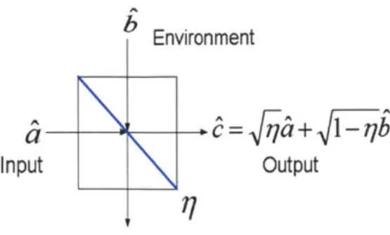
2-2 A single-mode lossy bosonic channel can be modelled as a beam-splitter with transmissivity rj. , is the input mode,

I

a

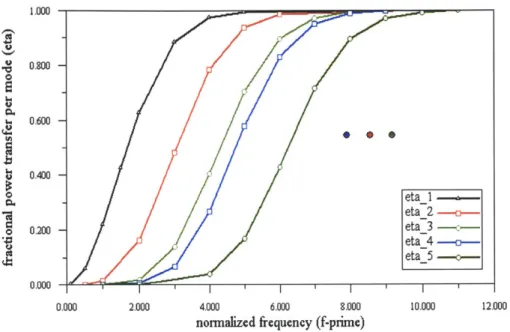
2-3 Variation of the fractional power transfers (transmissivities) of the first five successive spatial modes as a function of normalized frequency of transmission

f'

fc

frequency normalization. . . . . 21

3-1 Capacity (in bits per use) of the SM lossy number state channel com-puted for very low average input photon numbers, (a) Numerically

using the 'Blahut-Arimoto Algorithm' for q7 = 0.001 [blue solid line],

and (b) Using approximation (3.5) [black dashed line]. . . . . 33 3-2 Capacity achieving probability distribution for r/ = 0.2 and Ft = 2.62

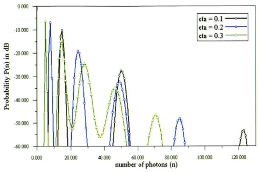
3-3 Capacity achieving probability distributions of photon numbers at the input of the SM lossy bosonic channel for three different values of transmissivity - = 0.1, 0.2, and 0.3 (the black, blue and green lines respectively). All three distributions correspond to the same average number constraint A = 2.62. As the transmissivity decreases, the peaks

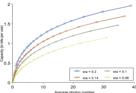
of the distribution spread out. . . . . 34 3-4 Capacity (in bits per use) CNS-DD(h), of the SM lossy number state

channel computed numerically using the 'Blahut-Arimoto Algorithm', and plotted as a function of h, for r7 = 0.2, 0.14, 0.1, and 0.06. . . . . 35

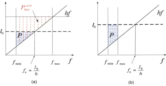
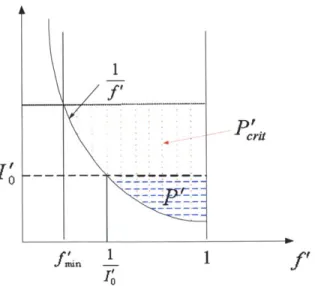
4-1 Optimal allocation of intensity across the transmission bandwidth to achieve maximum capacity on a lossless channel using coherent-state

4-2 This figure illustrates the effect of forced lower and upper cut-off fre-quencies (fmin and fmax), on the coherent state homodyne and hetero-dyne capacities. Given values of fmin and fm,, the critical power levels (the input power at which the critical frequency

f,

f

cases. In this figure, we plot the normalized capacities C' - C/fma

vs. a normalized (dimensionless) input power P' = P/hf2.. We normalize all frequencies by

fma.

f'

The 'dash-dotted' (black) line represents the capacity achievable using either homodyne or heterodyne with unrestricted use of bandwidth (Eqn. (4.20)), i.e. C = (1/ In 2) V2P/h bits per second. The 'solid'

(green) line, and the 'dashed' (blue) line represent homodyne and het-erodyne capacities respectively for any set of cut-off frequencies

satisfy-ing fi = 0.2. For this value of f'in P'd = 0.16, and P'h = 0.32.

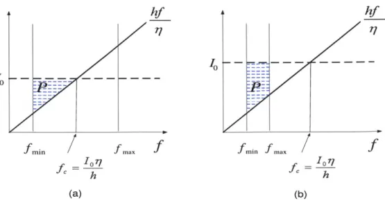
Different capacity expressions hold true for power levels below and above the respective critical powers (Shown by the thick and the thin lines in the figure respectively). . . . . 48 4-3 Optimal allocation of intensity across the transmission bandwidth to

achieve maximum capacity on a channel with frequency independent transmissivity TI, using coherent-state inputs and heterodyne detection.

(a) f

f , (b) fmax < fc. . . . .

.

.

. . . .

.

. . . .

51

achieve maximum capacity on a channel with frequency dependent transmissivity q OC

f2,

4-5 Dependence of C' on P' for coherent-state inputs and heterodyne

de-tection, for different values of

fi.

fi

the red (dotted) line is for

fAni

for

fj

fnin.

f'..

4-6 Dependence of C' on P' for coherent-state inputs with heterodyne and homodyne detection, for

f'

hetero-dyne detection, and the red (dashed) line is for homohetero-dyne detection. . 57

4-7 This figure illustrates the coherent state homodyne and heterodyne capacities for the free-space optical channel in the near-field regime. All the frequencies in the transmission range

f

>

2-1). Given values of fmin and fm,, the critical power levels (the input power at which the critical frequency

f,

fmax, and beyond which power 'fills up' only between

fmin

f

have been denoted by Phr and Ph, respectively for the two cases. The 'solid' (black and blue) line, and the 'dashed' (red and green) line represent homodyne and heterodyne capacities respectively for any set of cut-off frequencies satisfying

fj,1,

fmi,

values of the normalized critical input power are: p'crit = 0.019, and

p'it = 0.076 respectively. Different capacity expressions hold true for

power levels below and above the respective critical powers (Shown by the thick and the thin lines in the figure respectively). . . . . 62

4-8 An example of ultra wideband capacities for coherent state encod-ing with homodyne or heterodyne detection, for the free-space optical channel under the assumption of a single spatial mode transmission. . 65

4-9 The optimal power allocation for the wideband coherent state chan-nel with heterodyne detection depicted as 'water-filling', for frequency dependent transmissivity shown for ql in Fig. 2-3. . . . . 67 5-1 This figure shows comparative performance of squeezed state encoding

and homodyne detection with respect to that of coherent state encod-ing with homodyne and heterodyne detection. The 'solid' lines (red, green and grey) represent coherent state heterodyne, coherent state homodyne, and squeezed state homodyne capacities respectively for an arbitrary set of cut-off frequencies satisfying f' i= 0.2. Different capacity expressions hold true for power levels below and above the respective critical powers (Shown by the thick and the thin lines in the figure respectively). For the above value of

f'

nor-malized cut-off power are: P' = 0.32, p' = 0.08, and p'crit = 0.16.

The thick dashed (blue) line is the best achievable performance of the coherent state channel (with either heterodyne or homodyne detec-tion), and is given by C' = (1/ In2) 2P'. The thick dotted (red) line

is the best achievable performance of the squeezed state channel, and is given by C' = (1/In 2) 1. . . . . 73 5-2 An example of ultra wideband capacities for squeezed state channel and

coherent state encoding with homodyne or heterodyne detection, for the free-space optical channel under the assumption of a single spatial m ode transm ission. . . . . 75 6-1 Single Mode Capacities (in bits per use of the channel) for various

cases. The transmissivity of the SM channel q = 0.16. . . . . 78 6-2 Dependence of C' on P' for the ultimate classical capacity compared to

C' for coherent-state inputs with heterodyne and homodyne detection.

All curves assume f'is = 0. The blue (solid) line is the ultimate

classical capacity, the red (dotted) line is for heterodyne detection, and the green (dashed) line is for homodyne detection. . . . . 81

7-1 The thermal noise channel can be decomposed into a lossy bosonic channel without thermal noise (2.1), followed by a classical Gaussian

noise channel 4

(1 ,)F (7.4). . . . . 90 7-2 A plot of E' o Pn,k for a SM thermal noise channel with transmissivity

T = 0.8, and N = 5 photons, as a function of m; for n = 0, 6, 12, 18,.

The dark (black) lines correspond to the values n = 0, 30, 60, 90. . . . 96 7-3 A plot of output entropies of the SM thermal noise channel as a function

of 71 for number states inputs In)(n1, corresponding to n = 0, 1, 2, 3 and 4. The value of N = 5. We see that output entropy is minimum for

the vacuum state 10) (0 , which is shown in the figure by the dark black line. The results for n > 0 were obtained by numerical evaluation of the pa, from (7.18); the n = 0 entropy result so obtained matches the

analytic result g((1 - ,)N ). . . . . 97

7-4 A plot of optimum apriori probability distributions (in dB) for a pure

SM lossy channel (Tj = 0.8, h = 3.7), and a SM thermal noise channel

(T = 0.8, h = 3.7, N = 5). In the pure lossy case, there are no peaks

at this value of transmissivity and the distribution is close to linear, whereas for the thermal noise lossy channel, the distribution still has multiple peaks. For the optimum distribution of the thermal noise channel to converge sufficiently close to the Bose-Einstein distribution, y has to be even closer to unity. . . . . 102

7-5 A sample calculation of the number-state direct-detection capacity

(us-ing the Blahut-Arimoto algorithm) of a SM lossy thermal noise channel with transmissivity 7 = 0.8, and mean thermal photon number N = 5. 102

7-6 A sample simulation result of all the different capacities of a SM lossy

thermal noise channel we considered so far in the thesis. The channel SN has transmissivity y = 0.8, and mean thermal photon number N = 5.106

7-7 Ultra-wideband capacity of a lossy thermal noise channel - Free-space optical communication, single spatial mode propagation - AT = 400

cm2 and AR = 1 cm2, separated by

L

frequencies of transmission ranging from that associated with a wave-length of 30 microns (which is deep into the far-field regime), to that associated with a wavelength of 300 nanometers (which is well within the near field regime). Mean thermal photon number N = 5 is assumed

to remain constant across the entire range of frequencies. . . . . 108

7-8 Capacities of a wideband lossy thermal noise channel - Free-space

optical communication, single spatial mode propagation all param-eters same as in Fig. 7-7, except that the mean thermal photon number

N is now assumed to vary with frequency of transmission

f

to E qn. (7.2) . . . . 108 A-1 Blahut-Arimoto Algorithm . . . . 113

Chapter 1

Introduction

The objective of any communication system is to transfer information from one point to another in the most efficient manner, given the constraints of the available physi-cal resources. In most communication systems, the transfer of information is done by superimposing the information onto an electromagnetic (EM) wave. The EM wave is known as the carrier and the process of superimposing information onto the carrier wave is known as modulation. The modulated carrier is then transmitted to the des-tination through a noisy medium, called the communication channel. At the receiver, the noisy wave is received and demodulated to retrieve the information as accurately as possible. Such systems are often characterized by the location of the frequency of the carrier wave in the electromagnetic spectrum. In radio systems for example, the carrier wave is selected from the radio frequency (RF) portion of the spectrum.

In an optical communication system, the carrier wave is selected from the op-tical range of frequencies, which includes the infrared, visible light, and ultraviolet frequencies. The main advantage of communicating with optical frequencies is the potential increase in information that can be transmitted because of the possibil-ity of harnessing an immense amount of bandwidth. The amount of information transmitted in any communication system depends directly on the bandwidth of the modulated carrier, which is usually a fraction of the center frequency of the carrier wave itself. Thus increasing the carrier frequency increases the available transmission bandwidth. For example, the frequencies in the optical range would typically have

a usable transmission bandwidth about three to four orders of magnitude greater than that of a carrier wave in the RF region. Another important advantage of op-tical communications relative to RF systems comes from their narrower transmitted beams [tRad beam divergences are possible with optical systems. These narrower beamwidths deliver power more efficiently to the receiver aperture. Narrow beams also enhance communication security by making it hard for an eavesdropper to inter-cept an appreciable amount of the transmitted power. Communicating with optical frequencies has some challenges associated with it as well. As optical frequencies are accompanied by extremely small wavelengths, the design of optical components require completely different design techniques than conventional microwave or RF communication systems. Also, the advantage of optical communication derives from its comparatively narrow beam, which introduces the difficulty of high-precision beam pointing. RF beams require much less pointing precision. Progress in the theoreti-cal study of optitheoreti-cal communication, the advent of the laser - a high-power optitheoreti-cal carrier source the developments in the field of optical fiber-based communication, the development of novel wideband optical modulators and efficient detectors, have made optical communication emerge as a field of immense technological interest [1].

The subject of information theory addresses ultimate limits on communication. It tells us how to compute the maximum rate at which reliable data communication can be achieved over a particular communication channel by appropriately encoding and decoding the data. This rate is known as the channel capacity [20, 2, 31. It also tells us how to compute the maximum extent a given set of data can be compressed so that the original data can be recovered within a specific amount of distortion. Though information theory doesn't give us the exact algorithm (or the optimal code) that would achieve capacity on a given channel, and it doesn't tell us how to optimally compress a given set of data, nevertheless it sets ultimate limits on communication which are essential to meaningfully determine how well a real system is actually performing. The field of information theory was launched by Shannon's revolutionary 1948 paper [20], in which he laid down its complete foundation.

needed to assess the ultimate limits on optical communication. Much work has al-ready been done on quantum information theory [13, 4], which sets ultimate limits on the rates of reliable communication of classical information and quantum informa-tion over quantum mechanical communicainforma-tion channels. As in classical informainforma-tion theory, quantum information theory does not tell us the transmitter and receiver structures that would achieve the best communication rate for a given kind of quan-tum mechanical noise. Nevertheless the limits set by quanquan-tum information theory are extremely useful in determining how well available technology can perform with respect to the theoretical limit.

In this thesis, we will primarily focus on the lossy free-space quantum optical chan-nel. Some examples of such a channel are satellite-to-satellite communication, wireless optical communication through air with a clear line-of-sight between transmitter and receiver units, and deep space communication. Long distance communication through a lossy fiber or a waveguide can also be treated along similar lines. Quantum informa-tion theory work to date has not treated the lossy channel case sufficiently well. This thesis will establish ultimate limits achievable on reliable communication of classical information over such a channel. In addition, it will study the best possible per-formance of standard transmitter and receiver structures in relation to the ultimate achievable capacity. It will also consider the effects of background thermal noise on the ultimate capacity and other achievable capacities of the channel.

The organization of this thesis is as follows. In chapter 2, we elaborate the chan-nel model in detail, establish our notation for the rest of the work, present a short review on the notion of thermal noise in single mode bosonic communication, discuss some standard quantum detection schemes, and review the notions of unassisted and entanglement-assisted classical capacity of a quantum channel. The capacity of the far-field lossy channel using photon number state inputs and unit-efficiency direct detection receivers is dealt with in chapter 3. Chapter 4 evaluates the capacity of the lossy channel using coherent state inputs with homodyne and heterodyne receivers. The calculations in this chapter have been done for a simple frequency-independent loss model and for a more realistic free-space optical channel model in which the

transmissivity of the channel depends on the frequency of transmission, in both the near-field and the far-field regimes. We look into the achievable rates using optimized quadrature-squeezed state inputs in Chapter 5. We establish the ultimate classical capacity of a lossy far-field channel in chapter 6, and work out the single mode and wideband capacities in the presence of thermal noise, in Chapter 7. The thesis con-cludes in chapter 8 with a note on ongoing and future directions of research in the

Chapter 2

Background

This chapter is intended to provide all the necessary theoretical background and framework, with ample references to previous work in the area, for the material to be covered in the thesis. We discuss the model of the free-space quantum optical channel both in the far-field and the near-field propagation regimes. We describe the well known structured receivers for single mode (SM) bosonic states, and lay down their definitions mathematically. We also present a brief discussion on the notion of capacity for transmitting classical information over a quantum channel, followed by a discussion on entanglement assisted classical capacity. The chapter ends with a short note on the formulation of the power constrained wideband channel model that we use for all our subsequent capacity calculations.

2.1

Free-Space Propagation Geometry:

The Channel Model

Free-space optical communication has attracted considerable attention recently for a variety of applications [25, 26]. In the present work, we shall primarily focus on maximizing the rate at which classical information can be sent reliably over a free-space optical communication link under an average input power constraint by

AT

z-0 _AR

Free Space

z=L

Figure 2-1: Free space propagation geometry. AT and AR are the transmitter and receiver apertures respectively.

modes at the transmitter, and by using different detection schemes at the receiver. Consider a line-of-sight free space optical communication channel with circular shaped transmitter and receiver apertures denoted AT and AR respectively, as shown in Fig. 2-1. A quantized source of radiation at the transmitter produces a field E(r, t) which is space limited to the transmitter exit aperture AT

{

+y

and time limited to a finite signalling interval To = {t : to - T < t < to}. After

propagation through L m of free space, the field is collected by a receiver whose entrance aperture is AR {(x', y') :

+

{t

defined as Df = (ATAR/c 2

L2)f 2, where with some abuse of notation, we are now

using AT = irdo2/4 and AR = 7rdL2/4 to denote the aperture areas at the transmitter

and the receiver respectively. For narrowband transmission at a center frequency

f,

Environment

&

c =J0a+ 1-q~b

Input Output

Figure 2-2: A single-mode lossy bosonic channel can be modelled as a beam-splitter with transmissivity 7. e is the input mode, b is the environment, which remains

unexcited (in vacuum state) in the absence of any extraneous noise other than pure loss. is the output of the channel.

2.1.1

Far Field

In the far-field regime, only one spatial mode of the input bosonic field couples ap-preciable amount of power to the receiver aperture [5], and all other spatial modes are thus insignificant. Further, it has been shown that [5], in the Heisenberg picture, quantum description of the propagation of a single spatial mode of the field through this channel in the far-field regime is obtained by coupling the input field mode & into a beam splitter of transmissivity 7 = Df, with an 'environment' mode b (Fig. 2-2), which is in the vacuum state (2.1); i.e.

= d& + /1 - 7b, (2.1)

where

(ATAR

f 2

c2L2 )

₂₂

and d, , and b are the modal annihilation operators of the input, output and the noise modes respectively. Several authors like to call the above model a single-mode lossy

bosonic channel, where 1 - q is identified as the 'loss'. Physically, q is the fraction of the input power that gets coupled to the receiver aperture. Note that, q has a quadratic dependence on the carrier frequency

f

1.000 0 I-U 0.00 - 0.600-0.400 -0.200 -0.000 0.000 2.000 4.000 6.000 8.000

normalized frequency (f-prime)

10.000 12.000

Figure 2-3: Variation of the fractional power transfers (transmissivities) of the first

five successive spatial modes as a function of normalized frequency of transmission

f

772 > 773 > ... , and

f,

2.1.2

Near Field

As the value of Df increases, more and more spatial modes of the field start coupling appreciable power into the receiver. If we arrange the fractional power transfers of the spatial modes in decreasing order and denote the fractional power transfer of the ith mode by 7ij, then - from the eigenvalue behavior of the classical free-space modal decomposition theory [23, 24] - the qj's depend upon the carrier frequency

f

shown in Fig. 2-3.

When Df

>

modes which have e7 ~ 1, and all the other modes are insignificant [5].

eta_1 -eta_2 -eta_3 -eta_4 -eta_5

-0

.

2.2

Thermal Noise

In the absence of any extraneous noise sources other than pure loss, the environment mode b (2.1) is in the vacuum state, which is the minimum 'noise' required by quantum mechanics to preserve correct commutator brackets of annihilation operators of the output modes. Different types of noise can be described by different initial states of the environment mode 6. We define a thermal noise lossy bosonic channel to be a channel that describes the effect of coupling the lossy channel to a thermal reservoir

at temperature T [7]. The thermal environment mode 6 is excited in the state given

by the density matrix

PT

A

exp

-

a,

(2.3)

where 1a) are the coherent state vectors and S is the mean photon number per mode of the thermal state PT, given by the Planck's formula for the mean number of photons per mode of a blackbody radiation source at thermal equilibrium at temperature T:

N 1r~~uu) = = hf/JkBT -1 24

where h and kB are the Planck's constant and Boltzmann's constant respectively.

2.3

Quantum Detectors for Single Mode Bosonic

States

An arbitrary quantum measurement on a single EM field mode can be described in terms of a set of Hermitian operators {lb}, which satisfy

b ;> 0 (positivity), (2.5)

nib

These operators thus comprise a Positive Operator Value Measure (POVM). When field mode is in the state given by the density operator /a, the probability of an

outcome b is given by

Pr(bla) = Tr(I afb). (2.7)

Some of the basic quantum measurement schemes for single mode (SM) bosonic states that we will consider in this thesis are (a) Direct Detection, (b) Homodyne detection, and (c) Heterodyne Detection. Their POVM descriptions are given below

[6].

2.3.1

Direct Detection

Direct detection (or photon counting) refers to a widely used method of optical demodulation that responds to a short time averaged power of the optical field. Quantum mechanically, it refers to a measurement done in the number-state basis

{in),n

H = In)(ni, for n=0,1,2,... (2.8)

2.3.2

Homodyne Detection

Homodyne Detection refers to a quantum detection scheme in which the incoming field is mixed with a strong local oscillator (LO) field through a 50-50 beam-splitter (BS). The LO field is spatially and temporally coherent with the incoming field. The outputs of the BS are detected by two ideal photon counters. The output of the homodyne detector is the scaled difference of the output of the two photon counters. Homodyne detection measures one quadrature of the field in a given direction in phase-space, depending upon the phase of the LO-field. Homodyne detection can be

described by the POVM

where 11, are projection operators onto the 6-function normalized eigenstates lai) of the quadrature component ai = Re(a), that is in phase with the LO field whose phase, for convenience, has been set to zero.

2.3.3

Heterodyne Detection

Heterodyne detection refers to a simultaneous measurement of both the quadratures of the optical field. It mixes the received signal with a strong LO, whose center frequency is offset by a radio frequency -- known as the intermediate frequency (IF)

from that of the signal, on a 50-50 BS. Quadrature detection on the IF difference signal from photodetectors placed at the BS output ports then yields the desired measurements. Heterodyne detection can be described by the POVM

1

EH

= -c)(aL,

for aE

C,

(2.10)

7r

where 1a) is a coherent state.

2.4

Classical Capacity of a Quantum Channel

Let us consider an information source that emits discrete independent, identically-distributed (i.i.d.) classical symbols, indexed by i = 1,2,..., A. The source emits one letter at a time with a probability distribution PN, where PN(i) is the apriori probability that the symbol i is emitted. Our goal is to transmit the output of this source in the best possible manner over our quantum channel (2.1) using appropriate quantum states for encoding and an optimum detection scheme at the receiver. In particular, we wish to compute the capacity for transmitting classical information in bits, per use of a lossy quantum channel.

Let us assume that we excite the field mode & (in one signalling interval), in the quantum state ,i E 'R to encode the source-symbol i. Let us denote the state at the

output of the channel by <P(i) where the channel <P is a completely positive (CP) trace preserving map. A block code of length n would consist of codewords that in general

could be an entangled state 3 E Ro(n At the output, the most general quantum mechanical detection scheme can be described in terms of a POVM, which we shall call a 'decision rule' and denote by X = {X3}. Such a generalized measurement can be

thought of as a measurement of a quantity X whose possible results of measurement are labelled by

j

output symbols. The conditional probabilities that a particular output symbol is received given that a particular input symbol was transmitted through the channel, i.e. the classical transition probabilities [9, 11, 12] are given by

P(ji)

=

Tr(I(pA)X)

(2.11)

The classical mutual information and the quantum Holevo information for single use of this channel are respectively given by [13]

I(pN, (, X) = E pN()PJ log P(k) (2.12)

AH(PN =S (ZPN(i)i -E pN(i)S(i (2.13)

where S() = -Tr( log ,) is the Von Neumann entropy of the state 3. We define [13]

C (1) = sup sup I(pN, 4*", X) (2.14) {PNI X

C,(@)=

{PN(i)}

where (DO' = (D 0 4D 0 ... 0 1 represents multiple uses of the channel, and PN is a probability distribution over all states in H71. It can be shown that both of the above quantities are superadditive and that their averages with respect to n, as n -+ oc exist

[13]. From Shannon theory we know that, at any rate less than C(I), using product

state inputs over many uses of the channel to encode the source letters, one can achieve arbitrarily low error probability by using suitable classical coding techniques

[20]. We define CcQ to be the classical information capacity of a quantum channel 1 when the transmitter can encode messages using product state inputs and the receiver can decode using measurements entangled over arbitrarily many uses of the channel. The Holevo-Schumacher-Westmoreland (HSW) Theorem states that [13, 14].

CCQ = Ci(D). (2.16)

The ultimate capacity of a quantum channel 1 to communicate classical informa-tion is the supremum of the CCQ of n uses of ID (i.e. (pon), divided by n. We call this capacity the 'Classical Capacity' of a quantum channel, and denote it by CQQ or simply by C. The subscript 'QQ' signifies the fact that input-states and decoding can both be entangled over a large number of channel uses. So, the classical capacity of a quantum channel is

C = CQQ = sup (2.17)

n n

2.5

Entanglement-Assisted Capacity

A majority of the striking advantages that quantum information theory enjoys over

its classical counterpart stem from the wonders that quantum entanglement [4] can do to communication protocols. Teleportation and Superdense Coding [4] are two such examples. Surprisingly, it turns out that the classical information carrying capacity of a quantum channel can be increased way beyond its Classical Capacity

(2.17), by using prior shared entanglement as a resource. The entanglement-assisted classical capacity CE is defined to be the maximum asymptotic rate of reliable bit transmission with the aid of unlimited amount of prior entanglement shared between the transmitter and the receiver. The importance of CE lies in the fact that it gives an upper bound to all the relevant capacities of the quantum channel, including the quantum and classical (unassisted) capacities [21].

In can be shown [21] that the natural generalization of the concept of mutual information between input and output of a channel, to the quantum case, is given

by the Quantum Mutual Information I(, ,) of a quantum channel (D, where 3 is the

input state, given by

I(,y)

S()

+ S(I'())

-

S((W

0

T)PP)

(2.18)

where P is a purificationi of the input density matrix ,. It can be shown that the entanglement-assisted capacity CE is given by

CE=

max I(1,D)

(2.19)

where the maximum is taken over all possible inputs / to the channel [21].

2.6

Wideband Channel Model

The study of quantum limits to wideband bosonic communication rates has been one of the primary applications of quantum communication theory [15, 8]. The wideband capacity of a power-constrained lossless bosonic channel has been shown to be propor-tional to the square root of the total input power P [8]. Until very recently [18], the exact solution to the wideband classical capacity of the lossy bosonic channel was not known. In this thesis, we will demonstrate the calculation of the wideband classical capacities of the free-space channel (with and without thermal noise) for a variety of cases, viz. ultimate classical capacity, entanglement-assisted capacity, capacity achieved by using a coherent state encoding with heterodyne or homodyne detection, and capacity achieved by using an encoding based on an optimized set of quadrature squeezed states and homodyne detection. For all these cases, the procedure we use to compute the input-power-constrained wideband capacities from the respective SM

(bits per use) capacities is essentially the same. The procedure is illustrated below. Let us consider an input-power-constrained frequency multiplexed channel, in

'Purification of a mixed state is a purely mathematical process [4]: one can show that given any system A in a mixed state k^, it is always possible to introduce an additional reference system R and a pure state in the combined state space JAR), such that this pure state reduces to

yA

pA

Tr(IAR)(ARI).

which each frequency bin (of width b Hz) is in general a SM thermal noise chan-nel characterized by a transmissivity qi and an input-output relation similar to (2.1). In the following discussion, we shall consider communication using a single spatial mode of the bosonic field at each frequency

f

a real bosonic channel would primarily depend upon practical limitations on trans-mitter and receiver design, and on the optimum power allocation corresponding to the given set of transmitter and receiver structures. We denote the center frequency of the ith frequency bin by fi and use

bfih

the ith bin. The average input power constraint is then given by

P

b

hfiii.

(2.20)

In far field free-space propagation ,the transmissivity of the ith bin is ij = 2

where

A -

L2 _{(2.2). Let us denote by}

_Ri

photons in the ith bin of the environment;

Ni

f

fi.

denote the SM capacity (in bits per use) of the ith frequency bin by C(7i, fii, Si), then the wideband capacity CWB can be obtained as a function of the average input power constraint P, using a constrained maxization:

CwB(P)

=

MaxZC (qi(fi), fi,

(M)

(2.21)

subject to

b

hfig ; P.

(2.22)

The above maximization can be done using a Lagrange multiplier technique ei-ther analytically or numerically, depending upon the complexity of the SM capacity formula C

(rh(fi),

Note that this formulation assumes that different frequency bins are employed as parallel channels. Because of superadditivity, it must be shown that optimum capacity, for our channel, does not require entangling different frequency bins. Of

course, when seeking the capacity of specific transmitter-structure/receiver-structure combinations, we are free to assume that these structures do not entangle different frequency bins. In the subsequent chapters, we first work through the capacity cal-culations of all the different cases without thermal noise. We later summarize all the thermal noise capacity results together in one chapter.

Chapter 3

Capacity using Number State

Inputs and Direct Detection

Receivers

Number states are eigenstates of the photon number operator N = &f&, where d is the annihilation operator associated with a single mode of the bosonic field. The number state In) is the eigenstate associated with the eigenvalue of n photons. Clearly, as

N

{In);

counter) is a device that performs a measurement of N with unit efficiency, on an incident single mode (SM) field. If the state incident on such a receiver is the number state In), then the result of measurement is n with certainty.

3.1

Number State Capacity: Lossless Channel

Consider a zero-temperature SM lossless (rj = 1) bosonic channel (2.1), with a

max-imum average number of photons h, at the input. It is well known that classical capacity (2.17) can be achieved for this channel using photon number states and a unit-efficiency direct detection receiver [15]. The probability distribution of number states that achieves capacity is the Bose-Einstein distribution, given by

PN(n) =

1+h 1+h

where PN(n) is the probability of transmitting the state In)(nI in one use of the channel. The capacity (in bits per use) of this SM number state channel is given by

[15]

C(") = g(h) = log2(1+ "-1) + log2(1 + ). (3.2)

We also know that the ultimate classical capacity (in bits per second) of the wideband lossless channel with an average input-power constraint P (in Watts) is given by [15]

Cultimate(P) V

(3.3)

which can be achieved by number state encoding and direct detection [15]. In the rest of this chapter, we shall investigate the impact of loss on the capacities of SM and wideband channels with number state transmission and direct detection.

3.2

Number State Capacity: Lossy Channel

Let us transmit a pure number state PIN =

In)(nj

a zero-temperature SM lossy channel (2.1) with transmissivity 'q. It can be shown [4], that the output is a mixed state given by POUT = E'=o (nk(i - )n~kIk)(kI,

when we transmit In). If we detect this state using a unit-efficiency direct detection

receiver, the probability of getting m counts is (n)rp,(I - ' for m = 0, 1, 2,..., n. So, the classical transition probabilities (2.11) for a single use of the channel can be

written as

0 for m > n

3.2.1

SM Capacity

To get the SM capacity (in bits per use), we have to maximize the classical mutual information I(M; N) (2.12) over all input probability distributions pN(r) subject to a fixed value h of average photon-number at the input. This constrained maximization problem can be solved numerically using an iterative algorithm, known as the

Blahut-Arimoto

the special case Tpi << 1 (low-power, high-loss), some approximate analytical results can be obtained. In this regime, the SM capacity (in bits per use) of the number state channel is given by

C ~ H(7pi) - H(7), (3.5)

where H(x) X log2(x) - (1 - X) log2(1 - X) is the binary entropy function. The

results of a Blahut-Arimoto simulation for SM capacity in this regime has been com-pared with the above approximation in Fig. 3-1.

Interestingly, on carrying out the BA algorithm [16] for the general case, we find that the capacity achieving probability distributions have multiple peaks (See Fig.

3-2). This suggests that to achieve the best capacity using number state inputs, one

would almost preferentially use a set of optimum numbers of photons in each channel use. A sample plot of the optimal probability distribution for 7 = 0.2 and i! = 2.62

is given in Fig. 3-2.

A qualitative explanation of the appearance of these peaks in the optimum

dis-tribution is as follows. When photons are sent through the lossy channel in bunches of known magnitudes, the effect of the loss is to spread each bunch by some amount about its mean value. If the initial bunches are spaced out well enough, the pho-ton counting receiver is able to resolve them with little or no ambiguity. Thus, we should expect that the peaks of the probability distributions would space out more and more as we increase the loss (i.e., decrease the transmissivity 71), as lesser loss would imply lesser 'spread' of the peaks, and hence for the same level of 'ambiguity' at the receiver, we could afford to have the peaks closer together. Though the above

5.000e-4 4.000e-4 WI 3.2OOe-4 -1.000e-4 -1000 Approximation - -Blahut Arimoto -0-I- f I I I I I 0.000 0.020 0.040 0.060 0.080 0.100

Average Photon Number (nbar)

I 1

0.120 0.140

Figure 3-1: Capacity (in bits per use) of the SM lossy number state channel

com-puted for very low average input photon numbers, (a) Numerically using the

'Blahut-Arimoto Algorithm' for r

=

0.001 [blue solid line], and (b) Using approximation (3.5)

[black dashed line].

0 11111111

0 20 40 60 80

Photon number (n) 100

120 140 160

Figure 3-2: Capacity achieving probability distribution for r7

=

0.2 and A

=

2.62

photons.

i

i

I

A.

1

.

eta

I-

/

~{

I

\

f

\

V

*\

number

/

X

Figure 3-3: Capacity achieving probability distributions of photon numbers at the input of the SM lossy bosonic channel for three different values of transmissivity

--- 77 = 0.1,0.2, and 0.3 (the black, blue and green lines respectively). All three

distributions correspond to the same average number constraint ft = 2.62. As the

transmissivity decreases, the peaks of the distribution spread out.

explanation is not completely rigorous, this intuitive idea has been illustrated by ac-tual BA simulation results for the optimum distributions for 27 = 0.1, 0.2, and 0.3.

(Fig. 3-3). As one increases the transmissivity to unity, the multiple peaks in the optimum probability distribution gradually merge, and the distribution converges to the Bose-Einstein distribution (3.1).

Finally, a plot of the capacity (in bits per use) CNS-DD(!) as a function of h for various values of q is given in Fig. 3-4. As one would expect, for the same value of ii, the capacity increases with increasing transmissivity 71.

3.2.2

Wideband Capacity

The wideband capacity of the number state channel can be obtained numerically

by maximizing the sum of the SM capacities (obtained using the BA algorithm)

0.000

A

Ct

-60.000 0.000

2- 0.5-0 eta = 0.2 eta = 0.1 e eta = 0.14 eta = 0.06 0 10 20

Average photon number

30 40

Figure 3-4: Capacity (in bits per use) CNS-DD(5i), of the SM lossy number state channel computed numerically using the 'Blahut-Arimoto Algorithm', and plotted as

a function of h, for q = 0.2, 0.14, 0.1, and 0.06.

across the entire frequency range of transmission, subject to the average input power constraint P (Watts), using the Lagrange Multiplier technique described in Section

2.6. We will consider two cases (a) Constant high loss (frequency independent) and low input power at all frequencies; and (b) Frequency independent loss with arbitrary input power. The numerical analysis of the frequency dependent wideband far-field free-space channel turns out to be too complicated for the number state inputs.

Constant High Loss and Low Input Power

Let us assume that the total input power P is so small that the mean photon numbers fi < 1, Vi, where i is a discrete index corresponding to a narrow frequency bin of width b Hz centered at

fi

I

I

I

W = exp

[i+ AhI

f

,

where A is the Lagrange multiplier.

Substituting this result into the the power constraint equation (2.22), and ap-proximating the sums by integrals by assuming a vanishingly small bin width, we obtain

P

bh

fi

exp (-[ + Ohfi])

(3.7)

S Xe (3.8)

Ihf

-'(3.9)

eh021

where 3 = Aln 2/7, and allowing the integration to be over all frequencies is per-missible because the contribution of the optimum average photon number becomes

vanishingly small as f -- oc.

Substituting this relation into the capacity equation (3.5), and approximating the sums by integrals by assuming a vanishingly small bin width, we obtain

C

b

[H(pfi)

-

fiH(77)]

(3.10)

+ 71ln 77 + i(1 - 7) ln(1 - 7)]

[-ri 1n1 - qhi ln hi + (1 - 7nh) nh + ifn ln 77 - r77i (1 - I)]

In i In i (neglecting terms of second order in 71) (3.11)

3 (1 +

x)e-dx

Eliminating the Lagrange multiplier coefficient f from the power equation and the capacity equation, we obtain the wideband capacity CWB in bits/sec as a function of input power P:

CWB- 2T 2 P (3.13)

Note that in the limit of low power and high loss, the wideband capacity of a lossy channel with frequency independent transmissivity, achieved by number state encoding and direct detection, is proportional to the transmissivity 77.

Constant Loss with Arbitrary Input Power

Now, let us consider the general case of arbitrary transmissivity 77, without any re-striction on the input power constraint P. The analysis developed in this section can be used to compute the wideband capacity with frequency independent loss for any transmitter-detector combination for which the SM capacity (in bits per use) is known.

Let us set up the Lagrangian J(ni, A) as follows:

J(hi, A) = b C(, hi) + A(P - b hfih), (3.14)

where C(TI, hi) is the SM capacity in bits per use. Setting &J(nii, A)/Ohi = 0, we

obtain

____ - Ahfi. (3.15)

Oni

The above equation can be inverted to express hi as a function of Afi. Making the substitution z = Af, and converting the sums to integrals by going to the limit of vanishingly small bin width, we can define h(z) as a function with a continuous argument. Let us define a function m(z) = zn(z). Also, as we know C(rj, h(z)), we may express the capacity as a function of z, say C,,(z). Now, going through the algebra, one can show that the wideband capacity CwB satisfies

CWB, P fo

Cizdz

1

f" m(z)dz

Given the SM capacity, the term in the square braces is just a positive constant which can be evaluated easily. For rI = 0.2 for all frequencies, the capacity was cal-culated to be CwB,=0.2 = 0.5877/P/h, which is almost r7 times the lossless capacity

CWB,Iossless. So, similar to the 'low-power high-loss' case, at r7 = 0.2 with arbitrary input power P, the wideband number state capacity of the lossy channel (with fre-quency independent loss) is almost proportional to the transmissivity.

We later show that the ultimate classical capacity of the wideband lossy chan-nel C = V/CwB,ossIess, which can be achieved by a coherent-state encoding. So, one important conclusion is that - at least for the case of frequency-independent transmissivity - in contrast to the lossless case, number state encoding and direct detection is not optimal for the lossy channel. Another important observation from the above analysis is that, for frequency independent transmissivity, the wideband classical capacity of any lossy channel can be expressed as a constant times VP/h, where P is the constraint on total input power in Watts.

Chapter 4

Capacity using Coherent State

Inputs and Structured Receivers

Coherent states

{fla)}

ja)

= ala),

(4.1)

with, in general, complex eigenvalues {a}. The mean complex amplitude of the coherent state

Ia)

are the normalized quadrature operators. Coherent states are quadrature minimum uncertainty states each of whose quadrature components are uncorrelated and have variances ((A&i)2) = ((Aa2)2) = 1/4. One can derive the number-state expansion of a coherent state [15],

Ia) =

The two other properties of coherent states that we will use for our analysis are the inner product of two coherent states and the overcompleteness property: