A design methodology for hysteretic dampers

A Design Methodology for Hysteretic Dampers

by

Bora M. Tokyay

B.S., Lafayette College, PA (2001)

A.B., Lafayette College, PA (2001)

Submitted to the Department of Civil and Environmental Engineering

in partial fulfillment of the requirements for the degree of

Master of Engineering in Civil and Environmental Engineering

at the

MASSACHUSETTS INSTITUTE OF TECHNOLOGY

June 2002

@

Massachusetts Institute of Technology 2002. All rights reserved.

Author... ...

...

Department 'f AYvil and Environmental Engineering

May 15, 2002

Certified by ...

Professor of Civil

Accepted by ...

.

Jerome J. Connor

and Environmental Engineering

Thesis Supervisor

K

Oral Biiyiik6ztiirk

Chairman, Department Committee on Graduate Students

MASSACHUSETTS INSTITUTE OF TECHNOLOGY

J UN

3 2002

JUN

BARKER

A Design Methodology for Hysteretic Dampers

by

Bora M. Tokyay

Submitted to the Department of Civil and Environmental Engineering on May 15, 2002, in partial fulfillment of the

requirements for the degree of

Master of Engineering in Civil and Environmental Engineering

Abstract

In this thesis, a design methodology for hysteretic dampers, which are energy dissi-pation devices for buildings, is proposed. The increasing repair and insurance costs in the construction industry suggest a trend towards following a damage-controlled design philosophy in which the motion of the structure is the design parameter, as opposed to strength. Damage-controlled structures consist of energy dissipation sys-tems, such as hysteretic dampers, in addition to the primary structural elements. The proposed design methodology is developed and explained using a typical building and then evaluated by running computer simulations.

Thesis Supervisor: Jerome J. Connor

Thank you all. In order of appearance:

Mom and Dad - for getting it ALL started

My big brother - for being proud of me

achers at Robert College - for setting up the strong foundation RC'97 - for helping me be who I am

YAH'97 - for not letting me forget who I am Profs at Lafayette - for helping me get here Prof. Saliklis - for making me a structural engineer Friends at Lafayette - for making me have a great four years

MIT - for not being as bad as I thought you would be Special Thanks to...

nnor - for broadening my horizons and making me see the Big Picture Franny - for being and saying "canim benim"

Kevin - for too many things

Carmen - for our not "supposed to be had" conversations Fiona - for your sweet tone of speech

Marc - for understanding

Charisis - for being aaa, you know.... aaaa. He he he.. Tzu-Yang - for being the Master

Paul - for your valuable procrastination skills Lisa - for winning our love

Onur -- for the fresh food, the clean fridge, the clean room

a crazy nine-months here at MIT. Never thought I would be sad leaving but somehow you guys just managed to make me. Until we meet again,

enjoy, bora

Acknowledgments

Contents

1 Introduction 13

2 The Design Philosophy 15

2.1 Introducing Damage Controlled Structures ... 15

2.2 Establishing the Design Standard . . . . 17

2.2.1 Structural Performance Levels and Ranges . . . . 18

2.2.2 Seismic Hazard . . . . 19

3 Hysteretic Dampers 23 3.1 Applications of Hysteretic Dampers . . . . 23

3.2 How Do Hysteretic Dampers Work? . . . . 24

3.3 Recent Research on Hysteretic Dampers . . . . 27

4 Application Studies 31 4.1 Building Description . . . . 31

4.2 Strength Based Design . . . . 32

4.3 Design with Hysteretic Dampers: Method 1 . . . . 35

4.3.1 Conclusion . . . . 40

4.4 Design with Hysteretic Dampers: Motion Based Design Approach . . 41

4.4.1 Conclusion . . . . 45

5 SAP Analyses 47 5.1 Introduction . . . . 47

5.2.1 Assigning the "optimal" stiffness and damping values . . . . . 48

5.3 Results and Interpretation . . . . 52

5.4 What Went Wrong? . . . . 54

5.4.1 Expressing Hysteretic Damping as Equivalent Viscous Damping 55

5.4.2 The Earthquake . . . . 56

6 Cost Study 61

6.1 Cost of the Primary Lateral Support System . . . . 61 6.2 Cost of the Hysteretic Dampers . . . . 62 6.3 Cost of the Retrofit . . . . 64

7 Conclusion 65

A Los Angeles Ground Motion Records 67

List of Figures

2-1 Repair Costs vs Earthquake Intensity for Conventional and Damage-Controlled Structures. . . . . 16

2-2 Concept of Damage Controlled Structures: (a)Actual Structure; (b)Primary Structure; (c)Damping System. Taken from [8]. . . . . 17 2-3 Time history plots of the ground acceleration for Imperial Valley, 1940

earthquake and its BSE-1 and BSE-2 versions. . . . . 21

3-1 A hysteretic damper installed in a 44-story building . . . . . 26 3-2 Load-deflection curves for a yielding core element. . . . . 26 3-3 Idealized Hysteresis loop for an elastic-perfectly plastic material. Taken

from [5] . . . . 28

3-4 The unbonded-brace elements used in the Bennett Federal Building Project. Taken from [4] . . . . 29 3-5 Cross-section of an hysteretic damper proposed by KCI . . . . . 29

4-1 Floorplan and elevation views of the original structure. Taken from [3]

and [5] . . . . 31

4-2 The lumped-mass model of the original building with shear forces. . . 33

4-3 The chevron brace configuration used for the stiffness and hysteretic damper installations. . . . . 34 4-4 The modal shape of the original structure subjected to BSE-1. . . . . 37

5-1 The force experienced by the dampers is negligible, considering the dampers have a yield strength of 386.4 kips . . . . .

5-2 The dialog box in SAP2000 where the properties of are defined. . . . .

5-3 Maximum displacement observed on third floor vs. dampers for 50-50 stiffness distribution scheme. . . 5-4 Maximum displacement observed on third floor vs.

dampers for 30-70 stiffness distribution scheme. . .

5-5 Maximum displacement observed on third floor vs. dampers for 10-90 stiffness distribution scheme. . .

NLLink elements . . . . yield strength of . . . . yield strength of . . . . yield strength of

5-6 Time history of the force the hysteretic dampers (F, = 122.8 kips) in

the first story experience under BSE-1 excitation. . . . .

5-7 Time history of the force the hysteretic dampers (F, = 122.8 kips) in

the first story experience under BSE-2 excitation. . . . . 49 57 58 58 58 59 59

List of Tables

3.1 Tall steel buildings in Japan designed using hysteretic dampers. . . . 24

4.1 The mass of each story . . . . 32

4.2 Results of runs 1-6. . . . . 38

4.3 Results of Runs 7-10. . . . . 39

4.4 Number of iterations required for Runs 7-10. . . . . 40

4.5 Results of Runs 101-106. . . . . 44

5.1 Results of Runs 1-12. . . . . 53

A. 1 50/50 Set of Records (72 years Return Period). Taken from [3] . . . . 67

A.2 10/50 Set of Records (475 years Return Period). Taken from [3] . . . 68

Chapter 1

Introduction

The advances in the practice of earthquake engineering, coupled with the increased use of sophisticated computer analysis tools, have led engineers around the world to consider the use of energy dissipation devices in both large- and small-scale structures. These seismic energy dissipation devices are passive control devices that provide

re-liable sources of seismic energy absorption.

There are a number of energy dissipation or damping mechanisms currently avail-able for structural engineers. Some of the most common ones are viscous dampers, frictional dampers, tuned-mass dampers, viscoeleastic dampers and hysteretic dampers. The design methodology presented in this thesis is for hysteretic dampers. As such, hysteretic dampers will be investigated in greater detail in the following sections.

The use of damping mechanisms, hysteretic dampers in specific, to control the response of a structure is not limited to new buildings. In fact, the use of damping mechanisms in retrofit applications is gaining more popularity and acceptance ev-eryday. A good example to that is the Seismic Retrofit of the Wallace F. Bennett Federal Building in Salt Lake City, UT. Although the reinforced concrete structure was designed and constructed according to the codes that prevailed during its time of construction in the 1960s, the advances in seismic resistant design show that the building would not be capable of resisting the large magnitude earthquakes the nearby Wasatch Fault could generate [4]. The use of hysteretic dampers was found appropri-ate for that particular project considering parameters and constraints such as cost,

aesthetics and continuous functionality of the building during construction.

The Bennett Building is not the only structure that does not comply with the current building codes. In fact, the number of such structures is so large that Federal Emergency Management Agency (FEMA) funded a study to address this issue and arrive at feasible rehabilitation methods for such buildings. To achieve this goal, following a detailed investigation of numerous structures, FEMA identified several model buildings for analysis purposes according to parameters such as height and location.

In what follows, the concept of Damage Controlled Structures and the associated design philosophy will be introduced first. Following that, the thesis describes the mechanics of how hysteretic dampers work and then introduces three design method-ologies for retrofitting buildings with dampers. These methodmethod-ologies are applied to a three-story building located in Los Angeles to provide a basis for comparison. Although a rehabilitation strategy is the main interest of this thesis, the proposed design methodology is not restricted to retrofit applications and can be adapted for new buildings.

The optimal stiffness and damping combination from the Analyses section will be taken as inputs for the nonlinear analyses. The methods and simplifications used to model the structure and the associated difficulties that arose in the process are included to provide insight for further work.

The thesis concludes by addressing an important aspect of the rehabilitation pro-cess; the cost. The cost analysis is reduced to material cost calculations and finding the relative importance of each element in a rehabilitation project where hysteretic dampers are utilized.

Chapter 2

The Design Philosophy

2.1

Introducing Damage Controlled Structures

An optimal design for a building is the one that satisfies the predefined safety and serviceability requirements for the minimum amount of cost. Historically strength based design has been followed in practice. The current building codes, such as the Uniform Building Code, are based on the strength based design philosophy, in which the structure is designed with respect to strength constraints. The stiffness properties of the structure are established according to strength requirements, and then the building is checked for serviceability criteria. Usually an iterative process is necessary to obtain an acceptable design that satisfies both sets of requirements. This kind of design results in a structure in which the stiffness and energy absorption mechanisms are combined in one, as a result of which the building deforms inelastically.

Strength based design has been appropriate in the past where strength was the dominant design requirement. However, recent developments, especially the increase in repair and insurance costs suggest a new design philosophy should be used, one that minimizes the damage in the structure. Proposed by J. J. Connor1 _{and A. Wada}2

, a damaged controlled structure is "a combination of several structural systems and energy transformation devices that are integrated in such a way as to restrict damage

'Massachusetts Institute of Technology, Cambridge, MA

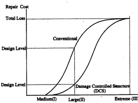
to a specific set of structural elements that can be readily repaired" [8]. The justifi-cation of using damage-controlled structure is depicted in Figure 2-1, taken from [8], which relates the repair cost to earthquake intensity for a conventional structure and a damage-controlled structure. The figure indicates that damage-controlled structures are most effective for moderate earthquakes.

Repair Co Total Loss Design Level

Design Level

Conventional

--- ---.--... .... _{Damage Controlled Sftctut} (DCS)

Medlum()

Large(U)

Figure 2-1: Repair Costs vs Earthquake Intensity for Conventional and Damage-Controlled Structures.

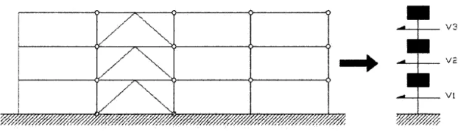
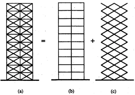
Since the main reason for damage is motion, creating a damage-controlled struc-ture involves controlling the motion of the strucstruc-ture. Connor and Wada argue in their earlier works [9], [7] that the spatial distribution of the structure's motion (i.e. the modal shape) is determined by stiffness, while the amplitude of the motion is a func-tion of both stiffness and energy absorpfunc-tion (or damping). Therefore in the design methods that are presented in this thesis as alternatives to strength based design, first the stiffness distribution that yields the desired displacement profile is obtained, and then the damping is added to adjust the magnitude of the response. It is worth remembering that the damping or energy absorption mechanism is separated from the primary system that provides both lateral and vertical support. Figure 2-2 depicts

the concept graphically. The structure (a) consists of (b) the primary structure and

(c) the damping system.

(b)

(c)

Figure 2-2: Concept of Damage Controlled Structures: (a)Actual Structure; (b)Primary Structure; (c)Damping System. Taken from [81.

2.2

Establishing the Design Standard

In October of 1997, Federal Emergency Management Agency (FEMA) released

FEMA-273: NEHRP Guidelines for the Seismic Rehabilitation of Buildings. This document,

which will be referred to as the Guidelines, is the latest and most appropriate stan-dard for any rehabilitation project. The Guidelines detail the requirements and steps of a systematic retrofit for a broad range of building types, performance levels, and seismic hazards.

One of the first steps in a rehabilitation process is to decide on a set of Rehabili-tation Objectives for the building. RehabiliRehabili-tation Objectives are "statements of the desired building performance when the building is subjected to earthquake demands of specified severity" [1]. Therefore in order to establish a set of Rehabilitation Ob-jectives, the structural engineer needs to know about Performance Levels and Seismic

(a)

-1-1-i-Hazard. Performance Levels Building performance can be described qualitatively in terms of several factors:

" The safety afforded building occupants during and after the event

" The cost and feasibility of restoring the building to pre-earthquake condition " The length of time the building is removed from service to effect repairs " Economic and architectural impacts on the larger community

In light of these factors, building performance levels and ranges are separated into two groups: Structural and Nonstructural. Since the main interest of this thesis lies in the structural problems caused by seismic excitations, the descriptions Performance Levels and Ranges are limited to those of Structural ones. In terms of notation, Structural Performance Levels are denoted by both names and numbers (following S-), while Nonstructural Performance Levels are identified by a name and an alphabetical designator (following N-).

2.2.1

Structural Performance Levels and Ranges

Three discrete Structural Performance Levels and two intermediate Structural Perfor-mance Ranges are defined. The Structural PerforPerfor-mance Levels are the Intermediate Occupancy Level (S-1), the Life Safety Level (S-3), and the Collapse Prevention Level

(S-5), while the Ranges are the Damage Control Range (S-2) and the Limited Safety

Range (S-4). Acceptance criteria are well defined for the levels, while design parame-ters for the ranges need to be interpolated from the values obtained for the preceding and the subsequent performance levels. The relevant Performance Levels and Ranges are explained below based on the definitions provided in the Guidelines:

Immediate Occupancy Performance Level (S-1)

The post-earthquake damage state in which only very limited structural damage has occurred. The basic vertical- and lateral- force resisting systems retain nearly all of their pre-earthquake strength and stiffness.

Damage Control Performance Range (S-2)

Continuous range of damage states that entail less damage than that defined for the Life Safety Level, but more than that defined for the Immediate Occupancy Level.

Life Safety Performance Level (S-3)

The post-earthquake damage state in which significant damage to the structure has occurred, but some margin against either partial or total structural collapse remains. There might be injuries during the earthquake, however life-threatening injuries are very unlikely.

Limited State Performance Range (S-4)

Continuous range of damage states between the Life Safety and Collapse Prevention Levels.

Collapse Prevention Performance Level (S-5)

The building is on the verge of experiencing partial or total collapse. Substantial damage is done to the structural systems, including degradations in strength and stiffness in vertical and lateral force resisting members. However, all significant com-ponents of the gravity-load-resisting system must continue to carry their gravity load demands. The structure may not be technically practical to repair and is not safe for reoccupancy, as aftershock activity could induce collapse.

For more detailed explanation of the Structural Performance Levels and Ranges as well as information on Nonstructural Performance Levels, the reader is advised to visit Chapter 2 of the Guidelines, [1].

2.2.2

Seismic Hazard

Seismic Hazard presents methods for determining earthquake shaking demands. Earth-quake demands are a function of the location of the building with respect to causative faults, the regional and site-specific geologic characteristics and the hazard level(s)

selected in the Rehabilitation Objective. In this study hazard levels defined on a probabilistic basis are used, which state the probability that more severe demands will be experienced (probability of exceedance) in a 50-year period. Hazard levels used in this study are given below:

Earthquake having probability of exceedance Mean Return Period (years)

50%/50 year 72 (rounded to 75) 10%/50 year 474 (rounded to 500)

2%/50 year 2475 (rounded to 2500)

In the Guidelines, and also in this thesis, frequent reference is made to two levels of earthquake hazard that are useful for the formation of the Rehabilitation Objective. These are termed Basic Safety Earthquake 1 (BSE-1) and Basic Safety Earthquake 2

(BSE-2). They are taken as 10%/50 and 2%/50, respectively. Appendix A includes

tables of basic characteristics of Los Angeles Ground Motion Records. Taken from

FEMA-355C, this table provides a set of earthquake excitations for the hazard levels

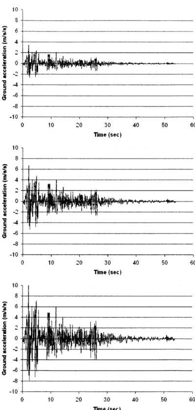
mentioned above. In the examples given in this thesis the Imperial Valley, 1940 earthquake is taken as the representative earthquake and is scaled up to a peak ground acceleration (PGA) of 261.0 in/sec2 _{(6.63 m/sec}2_{) for BSE-1. The same}

earthquake is scaled up to a PGA of 391.5 in/sec2

(9.95 m/sec2) to be used as BSE-2. Figure 2-3 shows the time history record of the acceleration for the Imperial Valley, 1940 earthquake as well as its scaled up versions corresponding to 1 and BSE-2. The time history data for this earthquake were obtained from the University of California, Berkeley Website.

Three levels of objectives are specified in the Guidelines, Basic Safety Objective (BSO), Enhanced Rehabilitation Objectives and Limited Rehabilitation Objectives. In order to achieve BSO the building rehabilitation must be designed to attain the Life Safety Performance Level for BSE-1 and the Collapse Prevention Level for BSE-2 earthquake demands. A structure that is retrofitted to provide a performance superior to BSO is said to have an Enhanced Rehabilitation Objective. Conversely if the goal of the retrofit is to provide a performance inferior to BSO, the Rehabilitation Objective is called Limited. It should be noted that structures designed and constructed in

0

Figure 2-3: Time history plots of the ground acceleration for Imperial Valley, 1940 earthquake and its BSE-1 and BSE-2 versions.

accordance with the latest building codes, namely BOCA 1993, SBCC 1994, ICBO 1994, may be deemed to meet the BSO.

Since the Guidelines provide a formal procedure to be followed only for BSO, it is suggested that according to FEMA attaining BSO should be the goal of a typical rehabilitation project. However, in light of Connor's and Wada's work on the sig-nificance and benefits of keeping the damage on the structure within economically repairable limits, and the definitions of the performance levels the BSO corresponds to, selecting BSO as the primary objective is deemed inadequate.

Therefore the Rehabilitation Objective set for this thesis consists of attaining Immediate Occupancy Performance Level for BSE-1 and Collapse Prevention Perfor-mance Level for BSE-2 excitation. This objective would be considered as an Enhanced Rehabilitation Objective, and is likely to cause higher initial costs. However it is ar-gued here that the initial higher costs will be offset by the savings in repair costs throughout the life of the structure.

The Guidelines have converted the qualitative descriptions of the Performance Levels into quantitative design criteria in terms of the allowable drift. According to these parameters, a structure consisting of Braced Steel Frames (which is the main structural system in the rehabilitated building in this thesis) can have 0.5% transient and negligible permanent drift for BSE-1 to satisfy the Immediate Occupancy Level and 2% transient or permanent drift for BSE-2 to satisfy the Collapse Prevention Level.

Chapter 3

Hysteretic Dampers

3.1

Applications of Hysteretic Dampers

To date, the use of hysteretic dampers has not been as popular in the United States as it has been in Japan, where this mechanism is used in more than 160 building [4]. However, there are reasons to believe its applications will gain popularity in the United States, especially in the seismic West Coast. Nippon Steel Corporation, the Japanese producers of the propriety low-yield strength steel used in the hysteretic dampers in Japan, are gradually entering the market in the West Coast. For instance, The Bennett Building, mentioned earlier in Section 1 is the first federally owned building to employ the buckling-restrained braces manufactured by Nippon Steel.

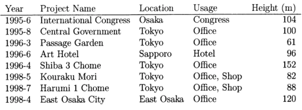
Table 3.1 below, modified from [10] lists some of the buildings in Japan where hysteretic damping systems are used. Two of the more interesting examples are briefly introduced below

Central Government Building

This 100 m high building serves as the headquarters for the Government Police Board and therefore has great importance. It is designed to behave elastically even under large intensity earthquakes. The hysteretic dampers used in this building are steel walls made of extra-low yield point steel (yield strength 10OMPa). The Hysteretic Damping system is accompanied by an additional viscous damping system which

Table 3.1: Tall steel buildings in Japan designed using hysteretic dampers. Year Project Name Location Usage Height (m)

1995-6 International Congress Osaka Congress 104

1995-8 Central Government Tokyo Office 100

1996-3 Passage Garden Tokyo Office 61

1996-6 Art Hotel Sapporo Hotel 96

1996-4 Shiba 3 Chome Tokyo Office 152

1998-5 Kouraku Mori Tokyo Office, Shop 82 1998-7 Harumi 1 Chome Tokyo Office, Shop 88

1998-4 East Osaka City East Osaka Office 120 consists of two movable steel plates and three fixed steel plates.

Passage Garden in Shibuya, Tokyo

This 61.4m building has 14 stories and no vertical columns. The entire structural system consists of two distinct systems; elastic column system and unbonded brace system (which provides hysteretic damping). The damage is clearly confined to the unbonded braces, which are installed in easy to replace locations.

3.2

How Do Hysteretic Dampers Work?

In pure frame elements (i.e. no braces, no dampers), the energy is dissipated through the yielding that occurs at the flange welded part of the beam ends for steel struc-tures [10]. In essence the beam ends are "sacrificed" for the structural integrity of the whole building. However, the yielding that occurs at the end of the beams is not enough to dissipate all the energy that enters the system and therefore large deformations are inevitable in case of seismic excitations.

Underlying the use hysteretic damping mechanisms is the same philosophy of sacrificing a member or members to avoid excessive damage in the building. Unlike in pure frames however, the yielding occurs in the core elements of the unbonded-brace members, which are usually installed diagonally in the chevron or V configuration. The design of such an element involves ensuring adequate yielding to absorb the

required energy.

To ensure that yielding occurs at the specified locations (i.e. at the hysteretic elements) and not anywhere else in the building, the core element of the damper is designed to have a relatively low yield strength in comparison to the primary structural elements. Currently all applications of hysteretic dampers use an ultra low yield steel produced by Nippon Steel, Japan as the core material. Although the use of low yield strength steel may be desirable with respect to yield considerations, the low buckling strength of the member is an unwanted consequence of such a selection. The fact that these members have low yield strength naturally leads to a buckling problem, since these members experience both tensile and compressive forces. That is why unbonded-braces are introduced.

Figure 3-1 shows a hysteretic damper installed by Mori Building Company of Japan in a 44-story building. The low yield strength steel core is encased over its length in a steel tube which is filled with concrete. The steel tube sleeve or jacket restrains the inner core from buckling by providing extra bending rigidity. However, a slip interface, or an "unbonding" layer between the steel core and the surrounding concrete is necessary so that all the axial force is taken by the core element. Hence the material and the geometry of the slip layer must be such that relative movement is allowed between the steel core and the concrete considering shearing and Poisson's effects, but at the same time buckling is prevented as the core member yields in compression.

The name hysteretic dampers comes from the behavior these yielding elements exhibit under cyclic loading. Figure 3-2 shows the Load-Deflection plot obtained from the testing of a material that is used as a yielding core element. In this particular example the curves are for ±0.4% and ±0.55% strain cycles. The loops that form are called Hysteresis loops, hence the name, hysteretic damper.

Extensive testing has been done both in University of California, Berkeley and Japan on unbonded-braces to produce repeatable symmetric behavior in tension and compression, up to ductility ratios of 15-20 [4], where ductility ratio is defined as the ratio of deformation at failure to deformation at yield. The advantage of the

Figure 3-1: A hysteretic damper installed in a 44-story building.

i-C

PIsn Had DWpmiqt (nhs)

Figure 3-2: Load-deflection curves for a yielding core element. 10

5

symmetric behavior for design purposes is that the element will be using its full capacity in both tension and compression. In traditional braces, where buckling is not prevented, the member is over-designed to avoid buckling, which means it has much more tensile strength than it needs. With the buckling-restraining system however, there is no need to over-design and members will utilize their full capacity, both in tension and compression. The test results indicate another advantage of unbonded-braces, namely the well-defined elastic-plastic bilinear behavior of the member. This allows for rational capacity design methods for the members.

3.3

Recent Research on Hysteretic Dampers

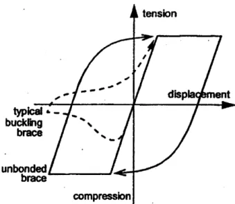
As mentioned in the previous section, hysteretic dampers absorb energy through yielding. Figure 3-3 shows an idealized axial load - displacement plot for an elastic-perfectly plastic material. The energy dissipated by the mechanism is represented by the area within the curve. Hence, more energy dissipation is achieved with increasing

F. (yield strength of the material), increasing ductility ratio or decreasing u,

(dis-placement at yield). This realization has triggered the use of hysteretic dampers as elements that become effective at higher level of excitations (high Fy). In other words for low levels of excitation the braces simply provide stiffness for the structure, while at high levels they yield and dissipate seismic energy.

This has been the methodology used most widely so far and hence the braces that are produced by Nippon Steel, Japan, are heavy and large as can be seen in the pictures included in this chapter. These braces have a steel yielding core, inside a steel jacket with concrete filling in the gap between the two steel components. Although this system performs its structural duties well, the use of these materials results in a heavy member, necessitating the use of machinery for installation.

It can be argued that if the installation of these members were easier and less costly they would be more widely accepted by the conservative construction industry that prevails in the United States. With that in mind, KaZaK Composites Incorporated (KCI) of Woburn, MA is working on different design schemes that would result in

tension

Figure 3-3: Idealized Hysteresis loop for an elastic-perfectly plastic material. Taken

from [5]

lighter brace elements, such that two construction workers without any machinery help could perform their installation. Some of KCI's findings are promising and are given below. It should be stated however that the axial force capacity of the braces KCI is planning to develop will not be as high as that of the larger and heavier ones produced by Nippon Steel. Therefore the target applications for these new designs are the rehabilitations of low-rise buildings. Hence, the investigation of the uses of these new devices is very fitting for the purposes of this thesis.

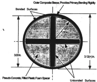
To solve the problem of heavy weight, KCI proposes the of use composite mate-rials for the anti-buckling sleeve and the spacer. Although the production cost may be higher, due to the use of composite materials, it can be argued that the savings incurred during construction will offset these extra costs. In that respect KCI inves-tigated several options before deciding on replacing the low yield strength steel core

by 1100-0 annealed aluminum [2]. This selection was due to its reported 5-7 ksi yield

strength and approximately 25% strain to failure. A major advantage of using 1100-0 aluminum as the yielding strut material is that its weight-specific energy absorption is approximately twice that of the Nippon Steel alloy (i.e. 2/3 the yield stress at 1/3

Figure 3-4: The unbonded-brace elements used in the Bennett Federal Building Project. Taken from [4]

the density). Replacing the steel buckling suppressing sleeve by a graphite/glass fiber sleeve and the concrete spacer by a foam spacer also results in weight reductions of about 70%. The resulting cross-section is shown in Figure 3-5.

- BondWd Surfacm

Unbonded Sufaces

Figure 3-5: Cross-section of an hysteretic damper proposed by KCI.

As stated earlier the findings so far are promising but naturally inconclusive. There are still many aspects of the issue that are unresolved, such as the connection details between the damper and the primary structure or the marketing of the new

product. Therefore KCI is continuing the investigation and testing with the help of outside consultants.

Chapter 4

Application Studies

4.1

Building Description

This thesis concentrates on the rehabilitation of a three-story special moment resisting frame (SMRF) originally developed for a series of nonlinear time history analyses in Phase 2 of the FEMA/SAC Steel Project [5]. The building is assumed to be in Los Angeles (seismic zone 4) on stiff soil (UBC soil type S2), and was designed to meet the 1994 UBC provisions. Figure 4-1 shows the plan view of the structure along with the geometry and the member sizes of one of the moment-resisting frames in the North-South direction of the building. It should be noted that grade beams were used at the foundation level to achieve full fixity of the column bases. All the columns in the perimeter of the building bend about their strong axes, which are oriented in the North-South direction. Further details of the building can be found in Appendix B of Reference [3].

A B C D E

-26

126

Mod MWIS W3WlO W2U44

1II

-AtIIkE

J

3-STORY I7'/7777777 /7777777 777777 77

Figure 4-1: Floorplan and elevation views of the original structure. Taken from [3]

and [5].

T

The designs of the moment frames are almost identical in the two orthogonal di-rections, therefore only half of the structure is analyzed. Also, the difference between the North-South (NS) and East-West (EW) is due to the difference in gravity load effects caused by the beams and sub-beams, since they are both oriented in the NS direction. However, because these load effects are negligible in moment frames, the analysis of the structure can safely be reduced to the analysis of only the NS direc-tion. Since only half of the structure is being analyzed the seismic masses, given as per floor values, were divided by two to obtain the values given in Table 4.1.

Table 4.1: The mass of each story Story mass(kips-sec2

/ft) mass(kg)

1 32.77 478,560

2 32.77 478,560

3 35.45 517,780

In accordance with the Rehabilitation Objective selected for this study, under

BSE-1 excitation the primary structure is to remain in the elastic range and have

a maximum drift of 0.5%, which corresponds to a maximum allowable shear strain

of 2,na = 1/200. Considering the height each floor the following design criteria are

obtained:

Maximum drift at the top, u* = 0.195 ft (0.06m)

Maximum allowable interstory drift, Au* = 0.065 ft (0.02m)

In what follows, three different design methodologies will be introduced and walked through step-by-step. Then these methods will be compared to each other in an attempt to identify the optimal one.

4.2

Strength Based Design

As mentioned in the Chapter 1, Strength Based Design is the design philosophy used in the current building codes. In order to understand the merits and disadvantages

of the alternative design methodologies this thesis proposes, one needs to attain an understanding of how Strength Based Design is performed and how the final structure behaves under the specified loads. In that respect, the building introduced in Sec-tion 4.1 is designed here according to the Uniform Building Code (UBC). However, chevron bracing is used to provide lateral stiffness, replacing the moment carrying frame system.

The strategy offered by UBC is to apply a quasi-static inertia force that is equiva-lent of an earthquake loading. The building is modeled as a simple beam with masses lumped at story heights, where these inertia forces are applied (see Figure 4-2). The shear caused by these inertia forces are then computed per floor along with the neces-sary stiffness to prevent extreme deformation. The cross-sectional areas of the bracing elements is calculated by taking into account the geometry (of the chevron brace) and

by assuming the brace is acting at the yield stress. The latter is a code criteria for

eccentric braced frames.

7 V3

V2

Figure 4-2: The lumped-mass model of the original building with shear forces. The shear force experienced by the first floor (base shear) is given as V = 0.099W, where W is the weight of the building. The base shear is proportioned and applied at each floor according to the weight of the stories above that particular floor. The obtained shear forces are increased by 50% as required by allowable stress design to obtain the following values:

I

Figure 4-3: The chevron damper installations.

brace configuration used for the stiffness and hysteretic

V2 = 326 kips

V3 = 170 kips

Following the design in Reference [5] the yield strength of the braces is taken as 34 ksi and is further reduced by 10%. Assuming the brace element acts at the yield stress, the area of each brace element is simply:

(4.1)

Ai = ^

0.9ory

where, F is the force each brace element experiences due to the shear on floor i. Taking 6 as the angle the brace makes with the horizontal(see Figure 4-3), and re-membering that there are two braces per floor, the force in each element is given

by:

F - i * - (4.2)

2cosO 1.31

These definitions yield to the following values of area for each brace element:

A1 = 12.05 in

2

A2 = 8.14 in

2

In order to see the response of the structure under certain seismic loads, the stiffness per floor was calculated using Equation 4.3.

A

2

ki = 2 (A )Cos2o, (4.3)

L i

The resulting stiffness values were then entered into MotionLab' No damping was assigned to the structure in this analysis as the design procedure followed in this section does not incorporate any damping. The low damping (i.e. 1-2%) provided

by the structural frame is ignored. k, = 1258 kip/in2 _{= 220 MN/M} 2

k2 = 850 kip/in2 = 149 MN/M 2

k3 = 442 kip/in2 = 77.4 MN/M 2

The displacement results from MotionLab indicated that the structure had deformed more than the allowable limit defined in Section 4.1. The maximum displacement observed on the third floor was u3 = 0.43 m, while the interstory displacement was Au = 0.15 m.

4.3

Design with Hysteretic Dampers: Method 1

As the first step, the building is modeled as a discrete shear beam with lumped masses (as calculated in Section 4.1) at story heights and varying lateral stiffness for each floor. The stiffness per floor was calculated using the following equations:

For interior columns:

12EIc

kint = 2~ (4.4)

h3(1 + r)

For exterior columns:

12EIc

kext = (4.5)

h3(1 + 2r) 1

MotionLab is a computer analysis software developed by J. J Connor. It analyzes lumped mass models (in the linear region) using conventional or modal state-space formulations. It allows the analyst to enter different values of mass, stiffness and damping values for each story.

where,

h: floor height

h Ib

E: Modulus of Elasticity

I, Moment of Inertia of the column

Ib: Moment of Inertia of the beam

Lb: Length of the beam

The calculations in Appendix B result in the following stiffness values:

k= 465 kip/in (81,440 kN/m)

k2= 411 kip/in (72,030 kN/m)

k3 = 188 kip/in (32,920 kN/m)

It should be mentioned that the bending deformation effects were neglected in these calculations since experience shows that low-rise buildings such as the one under investigation show a shear-beam response as opposed to a bending-beam response [6]. The modal shape observed when the original structure was subjected to BSE-1 excitation is given in Figure 4-4. Note that the modal shape gives relative values of displacement, not absolute, as the displacement of each node is normalized with respect to the maximum nodal displacement. Although the modal shape is close enough to the desired modal shape (i.e. constant interstory displacement) for the first mode the magnitude of the displacements, given below, are much higher than the design limits specified Section 2.2. These two findings were the basis for attempting to the bring the response of the building down to acceptable limits by applying damping to the system, without increasing the stiffness.

U3 = 0.75m (29.53in) Au = 0.25m (9.84in)

Modal displacement profile - real part - structure 3

-0.6 -0.4 -0.2 0

amplituc

0.2 0.4 0.6 0.8 1

Figure 4-4: The modal shape of the original structure subjected to BSE-1. Many simulations were run with various values of ca, (the damping coefficient per floor) with the objective of reducing the response. Results of some of the runs are tabulated in Table 4.2. These results indicate that additional damping causes considerable increase in the damping of the second and third modes, while, the modal damping for the first mode is not as sensitive to the changes in the ca, value.

Around c,=5 500 000 Ns/m an interesting phenomenon was observed. The modal periods and modal displacement profiles changed orders. As the value of the damping coefficient was increased even further the second mode became overdamped and the period of the second mode jumped up to around 600 seconds, which suggested that the solution blew up and should be discarded. This unexpected phenomena is worth investigating in greater detail. However, as it did not fit into the scope of this thesis, the problem was avoided by selecting c, values that were smaller than the limiting value. - First mode - Second mode - - Third mode -0 -0.8

Table 4.2: Results of runs 1-6.

Run# ca,(MN-s/m) .j1(%) 2(%) 3(%) Ti(s) T2(s) T3(s) u3(m) Au(m)

1 1.50 7.0 21.5 23.0 1.23 0.53 0.31 0.260 0.087 2 2.50 11.5 36.0 38.5 1.23 0.55 0.32 0.200 0.067 3 3.50 15.5 51.0 54.0 1.23 0.57 0.33 0.175 0.058 4 4.50 20.0 67.0 71.5 1.23 0.65 0.47 0.157 0.052 5 5.00 22.0 74.0 81.0 1.23 0.69 0.58 0.157 0.052 6 5.45 23.0 94.0 77.0 1.23 1.12 0.67 0.144 0.048 Change in Strategy

The initial strategy was to increase damping while keeping the stiffness constant until the response of the structure was decreased to the allowable values. The value of damping at which the structure's response was within the allowable values was going to be taken as the upper limit for damping.

However, the phenomenon observed around ca, = 5 500 000 Ns/m lead to a

modification of the strategy. Damping coefficient of 5 450 000 Ns/m was taken as the upper limit for damping and the stiffness values of each floor were adjusted. It should be noted however, that the value of 5 450 000 Ns/m was the limiting value for the damping coefficient, for the structure with no additional stiffness. As more stiffness was added to the structure, the value of 5 450 000 Ns/m for damping was no longer a limiting value and the overdamping of the second mode was avoided. The modified strategy is as follows:

1. For the first run, enter the original stiffness values (i.e. the stiffness of the

original building, ki's used in Runs 1-6) as the initial stiffness values, however utilize the "iterate on stiffness" option of MotionLab 2. As for the damping

coefficient value, use the upper limit value of c, = 5 450 000 Ns/m.

2. Record the displacement results.

3. For the subsequent runs, enter the original stiffness values as the initial stiffness 2_{The algorithm MotionLab follows consists of iterating on the stiffness values on a per floor basis}

until the displacements obtained are less than the design value. The outline of the algorithm can be found in Chapter 2 of [6].

values and click on the "iterate on stiffness" option, just like in Step 1. However, pick different ca, values depending on the results from the previous run. 4. Record the displacement values and repeat Step 3 as many times as necessary,

until the displacements converge on the design values.

The results of the runs following this procedure are listed in Table 4.3.

The results of Run 7 show that the structure's response is under the maximum allowable deformation. However, the values are considerably lower than the design values, suggesting the existence of a more efficient design (i.e. a stiffness and damping combination) that yields a response that is closer to the desired response. Just like in any design, an iterative process is followed after Run 7 by changing the damping values to obtain a response that is as close to the design response as possible.

Table 4.3: Results of Runs 7-10.

Run k1 k2 k3 Cay 1 2 63 U3 AU (MN/m) (MN/m) (MN/m) (MN-s/m) (%) (%) (%) (m) (m) 7 920 690 410 5.45 7.0 22.5 26.5 0.049 0.016 8 720 520 280 9.50 15.0 48.0 53.0 0.053 0.018 9 660 480 250 11.5 19.0 62.0 68.0 0.058 0.019 10 650 480 240 12.5 21.0 68.5 26.0 0.058 0.019

Since the structure was "too stiff" in Run 7 a higher damping coefficient value

(ca=9 500 000 N-s/m) is used in the next run, leading to smaller iterated stiffness

values. The resulting displacement values are once again considerably lower than the design values, hence value of the damping coefficient is increased once more to Ca,=

11 500 000 N-s/m in Run 9.

The results of Run 9 are "pretty good" and most likely adequate for preliminary designs. However, an additional run was completed as a way to check that the results really are converging on the design values. Although the displacement values obtained from Run 10 were indeed closer to the design values, the difference was negligible. It needs to be mentioned here that the controlling value for the iterations performed on the stiffness values is the interstory displacement. The iterations continue until

the average of the interstory displacements is equal to the design value, which in this case is 0.02m. If this happens to be an unsatisfactory or an inappropriate controlling criteria, then one can use the stiffness values from the previous run, modify them slightly and run a new analysis without iterations.

The results of Run 10 also indicate that increasing the damping coefficient to 12

500 000 N-s/m (8.6% increase) caused only a negligible decrease (1.4%) in the total

required stiffness of the building. This may be an important factor to consider for design since the magnitude of total stiffness and damping are related to the cost. This issue will be discussed in more detail in Chapter 6.

An additional factor that may be of importance is the number of iterations per-formed on the stiffness values for each run. Table 4.4 shows how many iterations were required to achieve the desired interstory displacement for each run. As one might imagine, the more the iterations, the higher the cost of calculations, especially for larger projects.

Table 4.4: Number of iterations required for Runs 7-10. Run

#

4.3.1

Conclusion

The results of this analysis shows that the original structure is extremely vulnerable to BSE-1 earthquake and that its stiffness is about a magnitude smaller than what it should be for the deformations to be acceptable. This confirms that moment frame systems do not provide much lateral stiffness, even when hefty members are used. In addition to being a moment frame, the relatively long bay widths, also caused the effective lateral stiffness to be small for this particular building.

for the optimal damping and stiffness values. Additional and sometimes considerable number of iterations were necessary afterwards for fine-tuning the response.

4.4

Design with Hysteretic Dampers: Motion Based

Design Approach

The design approach followed in Section 4.3 consisted of increasing the stiffness of the original building and adding damping to it until the desired response was achieved.

One can however, take a different approach to obtain close estimates to the stiffness and damping values directly. This method, which is explained below, is taken from

[6] and is named the Motion Based Design (MBD) approach. Similar to the previous

method, once the approximate values of optimal stiffness and damping are obtained, fine-tuning is necessary.

The starting point is the equilibrium equation for a damped system:

Mb*4+ C(D*q + KCD*q = P (4.6)

where, q is the displacement variable and the mass, M and the stiffness, K, matrices are given as:

M1 0 0 k1 +k2 -k2 0

M= 0 m2 0], K=

-k

0 0 M3 0 -k3 k3

where the subscripts denote the story number.

The * matrix is the desired modal shape. Since the desired modal shape for mode 1 corresponds to a constant interstory displacement, * is given as:

1/3

* = 2/3 (4.8)

The construction of the damping matrix, C depends on how the designer wishes to vary the damping throughout the structure. In this study, damping is distributed uniformly between the three floors, i.e. every floor has the same damping coefficient,

Cay. For this type of damping distribution the C matrix has the same form as the K

matrix:

C1 + C2 -C2 0 2Cav -Cav 0

C [-C2 C2 + C -C3 = cav 2Cav -Cav (4.9)

0 -C3 C3 0 -Cav Cav

Since in seismic excitations the nodal forces are proportional to the nodal masses, the force matrix, P is defined as:

MI

P = -ag m2 (4.10)

M3)

where mi are the floor masses and ag is the ground acceleration. Multiplying Equation 4.6 by (<D*)T yields:

in-4 + q +

Iq

where the quantities with superscript tilde are equivalent one degree of freedom mass, damping, stiffness and force quantities. They are defined and calculated as:

i = ()*)TM(* = 7.836 x 105kg (4.12)

a

kW2fn (4.14)

S=(lt*)Tp (4.15)

j is usually expressed in terms of the equivalent mass, ?'n- and the modal participation factor, F, as:

where,

r

M (4.17)

Using these definitions and results, the stiffness for each floor is obtained. During the process one utilizes the response spectra shown in Figure 4-5. Since the maximum

100 E I 101 5 10 -10, 101 -- - - ...I .. . -. - . .. . ... .. ... . .. .. . . .. . . .. . .: ... -... ..

~~~~-

~ ~

~~~~~~~~~ ~ ~ ~

~

~

~

~

~~~~-

Figure 4-5: Response Spectra for BSE-1.

allowable maximum displacement is u* = 0.06m at the top, from the response spectra, one can obtain what the period of the structure should be by assuming a damping ratio for the system. However, since response spectra plots are for SDOF systems, one uses the modal participation factor F to express the current 3-DOF problem as a SDOF problem. Hence, the design spectral displacement is:

S = -U3 = 0.0467m (4.18) In this study the stiffness calibration was based on a damping ratio of, = 20%. This damping ratio along with the maximum allowable shear deformation lead to a

struc-ture with a period of T = 0.50 seconds (from Figure 4-5). The stiffness distribution that yields that period value is:

472

k = 396 x 106N/m (4.19)

245)

The damping coefficient per floor is obtained by:

c = 2w&n = -cay (4.20)

3

cay = 11.8 x 106N-s/m (4.21)

These values of stiffness and damping should theoretically yield a response that is equal to the design limit. As a check these values are entered into MotionLab, the response is observed and modifications are made in a fashion similar to the method of Section 4.3. Results of these runs, Runs 101-106 are listed in Table 4.5.

Table 4.5: Results of Runs 101-106.

Run k, k2 k3 Cay ' 2 3 U3 AU (MN/m) (MN/m) (MN/m) (MN-s/m)

(%) (%)

During Runs 101-103 the limiting value for the damping coefficient was found to be cav=13 000 000 N-s/m. On Run 103, the iteration function was selected, so that the stiffness values would be iterated until an interstory displacement of Au = 0.020m is obtained. However, results of Run 103 and some intermediate runs that are not given here, showed that the iterations caused the building to be too stiff. Therefore in Runs 104 to 106 manual iterations were performed based on the result of the previous run, until the desired response was achieved.

4.4.1

Conclusion

In the MBD approach stiffness and damping values that yield approximately the design deformations are obtained initially following a simple algorithm introduced above. Then, several manual "iterations" are necessary to achieve the design criteria. The main difference between MBD approach and approach of Method 1 is the amount of flexibility (and hence responsibility) given to the designer. The designer needs to be able to interpret the results of a run properly in order to make the necessary modifications on certain parameters for the next run. In addition, the number of iterations required in Run 103 was only one. Attaining an approximate value for stiffness using the MBD approach required less iterations. Again this may have significant impact on the cost of the calculations for larger scale projects.

Chapter 5

SAP Analyses

5.1

Introduction

In Chapter 4, three design methodologies were presented, one being the more tra-ditional Strength Based Design. The latter two methodologies are associated with damage controlled design and introduce stiffness and damping to the structural sys-tem. In this chapter the optimal design values obtained in Chapter 4 will be input into SAP20001 to observe the structure's response under BSE-1 and BSE-2 loadings. Since the Performance Level to be used for design purposes allows the structure to enter the nonlinear region under BSE-2 loading, the use of SAP2000 Nonlinear was necessary.

It was previously shown, in Section 4.2 that the structure resulting from the Strength Based Design would experience unacceptable deformations even under

BSE-1 loading. Therefore, that design approach is discarded. Although the remaining two

methods were very similar in nature the results of the Motion Based Design Approach will be used here simply because it is the approach that provided the designer with more flexibility and responsibility during the process.

1A widely used finite element structural analysis program produced by Computers & Structures, Inc.

5.2

Input

The first step in the SAP2000 analysis was to enter the geometry of the building and then to assign sections to the frame members in accordance with the original building. After this was completed the two loading Time History Functions and Cases were defined for the BSE-1 and BSE-2 excitations.

Then the retrofit began, i.e. the additional stiffness and dampers were installed using the chevron brace configuration. Both the braces that provide the stiffness and the damping elements were defined as NonLinearLink (NLLink) elements, as discussed in the next section. For analysis purposes that the dampers and the main lateral stiffness members were placed in different bays for reasons of clarity2. During actual construction the location of these elements would be governed by other factors, such as accidental torsion effects. It should be noted however, there is no reason for the dampers not to be put in the same bay as the braces that provide stiffness. How the necessary properties for the stiffness and damper members were obtained and entered into SAP2000 are explained next.

5.2.1

Assigning the "optimal" stiffness and damping values

From the results of the Motion Based Design approach required stiffness and damping values per floor are given as:

k

k2 = 440 MN m = 2512 kip/in

k3 = 330 MN/m = 1884 kip/in

The first thought that comes to mind is to provide the total floor stiffness by the brace elements, which are the traditional braces using normal 36ksi steel, and add the dampers totally separately. The dampers themselves would be providing some lateral

2_{The analyses were performed using only a two bay structure, rather than the four bay structure.}

This simplification could be made, since eliminating the additional stiffness provided by the bending of the members in the other bays lead to a more conservative analysis.