The Design and Testing of a Procedure to Locate Fresh
Submarine Groundwater Discharge in Cyprus
by
Kathryn M. Olesnavage
SUBMITTED TO THE DEPARTMENT OF MECHANICAL ENGINEERING IN PARTIAL FULFILLMENT OF THE REQUIREMENTS FOR THE DEGREE OF
BACHELOR OF SCIENCE IN MECHANICAL ENGINEERING
AT THE
MASSACHUSETTS INSTITUTE OF TECHNOLOGY MASSACHUSEiINTITUTE
OF TECHNOLO y
FEBRUARY 2012
AR
22© 2012 Massachusetts Institute of Technology. All rights reserved. ARCH/S
; 4 1 "% '.1 /1 7- A
Signature of Autho
ri/
Department of Mechanical Engineering January 24, 2012
/
/)
Certified by:ID
Doherty Chryssostomos Chryssostomidis Professor of Ocean Science and Engineering Director of Sea Grant College Program-esis Supervisor
Thesis Supervisor Accepted by:
John H. Lienhard V Professor of Mechanical Engineering
The Design and Testing of a Procedure to Locate Fresh Submarine
Groundwater Discharge in Cyprus
by
Kathryn M. Olesnavage
Submitted to the Department of Mechanical Engineering on January 24, 2012 in Partial Fulfillment of the Requirements for the
Degree of Bachelor of Science in Mechanical Engineering
ABSTRACT
The aim of this collaborative project between Massachusetts Institute of Technology (MIT) and Cyprus Institute was to develop an experimental procedure for identifying fresh submarine groundwater discharge (SGD) in Cyprus. SGD is a flow of water from coastal aquifers into the ocean driven by a hydraulic gradient and other forces. Understanding SGD is crucial for informed groundwater management. In some cases, SGD creates submarine springs which can be tapped to provide supplementary freshwater. This is particularly enticing for countries such as Cyprus, where energy- and cost-intensive desalination plants are necessary to meet freshwater demand.
A preliminary protocol for locating SGD was developed based on a review of literature and
interviews with experts. The protocol was tailored to suit resources available in Cyprus. Because groundwater temperature typically deviates from ocean water, an infrared camera mounted on a manned aircraft was used to obtain an ocean surface temperature map. Areas exhibiting temperature anomalies were revisited by boat to measure salinity in situ using a conductivity, temperature and depth sensor
(CTD). This protocol was tested in Chrysochou Bay, selected based on relatively high estimates of SGD
from published water mass balances as well as recommendations from local fishermen.
The designed method proved effective; areas of anomalous salinities and temperatures were found. However the protocol can be improved based on experience gained through this study. Manned aircrafts are unfit for a large-scale study due to high costs, flight restrictions, and lack of appropriate navigational equipment on accessible vehicles. Unmanned aerial vehicles are more suitable for a full-scale study. Additionally, obtaining a salinity profile by a series of point measurements, as with the CTD, is time-consuming. A towed resistivity array would provide similar salinity profiles in a fraction of the time.
A thorough investigation of SGD is planned in Cyprus in the spring, when SGD is highest. This
paper presents a recommended procedure for the spring investigation based on the results of this study.
Thesis Supervisor: Chryssostomos Chryssostomidis
Title: Doherty Professor of Ocean Science and Engineering, Director of Sea Grant College Program
ACKNOWLEDGEMENTS
The author would like to first and foremost thank her advisor, Prof. Chryssostomos Chryssostomidis, for his continuous support and advice throughout this investigation, as well as for providing her with this amazing opportunity, and Prof. David Marks for his encouragement.
A special thanks also to Prof. Harold Hemond and Prof. Franz Hover from the Massachusetts
Institute of Technology as well as to Dr. Matthew Charette from Woods Hole Oceanographic Institute, all of whom were consulted on some aspect of the project. She is also grateful for everyone in the Sea Grant College Program for being so helpful and welcoming over the past year and to her wonderful friends and family for everything.
Additional thanks go to everyone at the Cyprus Institute, particularly Dr. Costas Papanicolas, Dr. Manfred Lange, Dr. Leonard Barrie, Dr. Adriana Bruggeman, Dr. Nick Polydorides, Dr. Cecelia Hannides, Ms. Eroulla Cadd, and especially Dr. Stelios Ioannou and Dr. Christos Keleshis for their daily assistance and hospitality. Thank you also to the pilots, Mr. Marios Argyrides and Mr. Constantinos Savvides, and the boat captain, Mr. Pavlos Hadjiantonis.
None of this research would have been possible without the financial support of the Cyprus Program at MIT through the Cyprus Research Promotion Foundation, the MIT Sea Grant College Program under NOAA Grant NA100AR417, and the MIT Energy Initiative. Thank you all so much for your kindness and generosity.
Table of Contents
1. Introduction ... 9
2. Background... 10
2.1 Subm arine Groundwater Discharge... 10
2.2 SGD as an Exploitable Source of Freshwater... 12
2.3 M ethods of Identifying and M easuring Freshwater SGD ... 12
2.3.1 Hydrogeological Calculations ... 12
2.3.2 Aerial Therm al Im aging ... 14
2.3.2.1 Infrared Thermography ... 14
2.3.3 Salinity... 15
2.3.4 Geochem ical Tracers ... 16
2.3.5 Lee-Type Seepage M eters ... 16
2.3.6 Other Observable Signs of SGD ... 17
2.4 Subm arine Groundwater Discharge in Cyprus ... 18
2.5 Proposed Procedure for Cyprus ... 20
3. Testing in Quonochontaug Pond, RI ... 21
3.1 Salinity Profiling ... 22
3.1.1 Conductivity, Tem perature and Depth Sensor... 22
3.1.2 Determ ination of M easurem ent Locations ... 24
3.1.3 Point M easurem ents of Salinity and Temperature... 25
3.2 Quonochontaug Pond Results and Discussion ... 26
4. Testing in Cyprus... 27
4.1 Procedure ... 28
3.1.1 Salinity M easurem ents... 28
4.1.2 Aerial Im aging ... 29
4.1.2.1 Infrared Video Camera... 29
4.1.2.2 Cloud Cap Technology Gim bal ... 31
4.1.2.3 Relating Infrared Images to Temperature Differences ... 33
4.1.2.5 Aerial Imaging Procedure ... 36
4.1.2.6 Video Post-Processing Procedure ... 37
4.2 Results and Discussion ... 37
4.2.1 Salinity... 37
4.2.2 Therm al Im aging ... 40
5 .C on clu sion s... 4 8 R eferen ces... 5 0
Appendix A. Using Google Earth to Find Waypoints... 52
Appendix B. Using MATLAB to Create Profiles from YSI CastawayTM -CTD ... 55
Appendix C. MATLAB Functions for YSI CastAwayTM -CTD Data Analysis... 69
Appendix D: Salinity Measurements from Quonochontaug Pond ... 83
Appendix E: Finding Anomalies in Grayscale Infrared Video with ImageJ... 84
Appendix F: Creating an Overlay from ViewPoint Snapshots in Google Earth ... 91
Appendix G: MATLAB Code for createMosaic Program ... 98
Appendix H: Creating a Google Earth Overlay for Any Image Using MATLAB... 100
1. Introduction
In the last several decades, Cyprus has struggled to meet the water demand for the country. Nearly all of the island country's aquifers have a history of being over-pumped, often leading to salt water intrusion and depletion. In the last decade the government has been forced to turn to expensive desalination plants that have a substantial environmental impact to solve the water deficit. While the current state of the nation's groundwater resources is relatively good compared to past years thanks to higher than average rainfall and the desalination plants, investigation of submarine groundwater discharge (SGD), an as of yet nearly untouched subject in Cyprus, would help inform future coastal water management decisions and could even reveal untapped freshwater resources.
SGD is the flow of water from a coastal aquifer into the ocean. It can be composed of either
fresh or salt water. This study focuses on freshwater SGD. While it usually occurs as slow, diffuse flow across sandy sediments, in confined karstic or rocky aquifers discharge can emanate from a single point source, creating submarine freshwater springs. These have been observed in many countries surrounding Cyprus (Fleury 2007, Taniguchi 2002, Elhatip 2003, Gunay 1988, Ghannam 1998). In some cases these springs have even been tapped and used as a supplemental source of freshwater.
Prior to this study, the only information about SGD in Cyprus came from equations describing groundwater flow and estimations of relevant parameters. The Cyprus Institute in Nicosia has proposed a full scale experimental investigation of SGD to be carried out in the spring, when precipitation and, consequently, SGD are highest. Before this investigation, an experimental protocol specific to Cyprus needs to be developed and refined so that no time is wasted in the spring, when time is a valuable commodity before summer hits, bringing with it dry weather.
The purpose of this project is threefold: a) to develop an experimental procedure based on a review of literature to locate SGD that can be carried out in Cyprus, b) to test the experimental procedure, and c) to provide recommendations for the next investigation based on the experience of testing the procedure.
Presented within this report is a summary of the information gathered from a review of literature on SGD and an explanation of the procedure developed for Cyprus based on this information. The results are provided from testing the procedure, both in Quonochontaug Pond, Rhode Island, where prior studies showed evidence of SGD, and then in Chrysochou Bay, Cyprus. Finally the experience of carrying out the procedure is described and recommendations are made for a future iteration of this project.
2. Background
2.1 Submarine Groundwater Discharge
All aquifers that come in contact with the sea have a dynamic freshwater - salt water interface; it can move either in towards land or out towards the sea when acted on by a number of forces. The position of this interface can allow water to flow from the ocean into the aquifer (salt water intrusion) or from the aquifer into the ocean (SGD).
Burnett defines submarine groundwater discharge as "any and all flow of water on continental margins from the seabed to the coastal ocean, regardless of fluid composition or driving force" (Burnett 2003). It can be caused by many factors and composed of freshwater from the aquifer, recirculated sea water, or a combination of the two. In aquifers with a porous top stratum (semiconfined aquifers) usually occurs as a slow, diffuse flow through the sediment. In coastal aquifers with karstic or rocky outcroppings, a crack can cause SGD from a point source that can create submarine springs.
Examples of driving factors of SGD include a hydraulic gradient, tidal pumping, wave set-up, density gradients, thermal gradients, and topography (Bratton 2010, Burnett 2003). Because the motivating forces behind groundwater discharge are many and often work together to influence groundwater flow, SGD is temporally and spatially variable, which complicates efforts to locate and understand it.
Bratton distinguishes three scales of SGD: the nearshore scale, which extends approximately
10 m out from the shoreline, the embayment scale, which covers the area from the first confining
unit to the 10 km from shore, and the shelf scale, which includes the entire continental shelf (Bratton 2010). Fig. 1 shows each of these scales.
Figure 1: Bratton separates submarine groundwater discharge (SGD) into the nearshore
scale, embayment scale, and the shelf scale. Reproduced from Bratton (2010)
Before understanding these scales, it is important to know what is meant by confined and unconfined in the context of groundwater. A confined, or artesian, aquifer is enclosed by impermeable surfaces on all sides, such as rock or karst. Confined aquifers often have high internal pressure. Fissures or cracks in the boundaries of a confined aquifer can result in water flowing out and above the water or ground level. The top of an unconfined, or phreatic, aquifer consists of highly permeable soils. Often aquifers are layered such that the bottom stratum of an unconfined aquifer is the top confining unit of a confined aquifer. An aquifer is semi-confined if the top layer has a low permeability.
The nearshore scale includes the intertidal zone and is linked to shallow, unconfined aquifers and topographically driven surface flow. It is the most studied and understood scale of
SGD. The embayment scale can feature diffuse seepage or point source discharge of freshwater,
potentially in substantial amounts. Because the groundwater at this depth will have had to travel further, it is often relatively pure. Shelf scale SGD can include many confined aquifers and is driven primarily by geothermal convection.
Understanding SGD is crucial in the study of coastal ecosystems, nutrient and contaminant transport, groundwater management, and freshwater conservation. The primary factors motivating this study are groundwater management and freshwater conservation.
2.2 SGD as an Exploitable Source of Freshwater
When groundwater discharges from a point source, it can create a submarine spring. Greek and Roman folklore tell stories of sailors reaching over the side of a boat miles from shore and pulling up a glass of water fresh enough to drink. Other accounts tell of collecting freshwater from off shore to bring back for use on land. Pliny the Elder (ca. 1't century A.D.) is quoted by Burnett as having written of "springs bubbling freshwater as if from pipes" in the Black Sea (Burnett 2003). Modern technology has allowed these springs to be tapped and used to supplement other sources of freshwater.
2.3 Methods of Identifying and Measuring Freshwater SGD
Many different methods of measuring SGD both qualitatively and quantitatively have been tested and proven capable. The spatial and temporal variability of SGD make it particularly important to use a variety of these methods to fully characterize SGD in the area of interest. Each of these methods has its own advantages and limitations which make them more or less applicable for a given situation.
2.3.1 Hydrogeological Calculations
Hydrogeological calculations are often performed as a first step in estimating SGD quantitatively. These calculations give no indication of location of SGD or of variations in
behavior of discharge with space or time, but do provide a quick means of estimating the amount of water outflow to an ocean from a particular aquifer. Two equations can be used to approximate SGD: Darcy's Law and water mass balance.
Groundwater flow rates are governed by Darcy's Law, which describes the rate at which water flows through a porous medium. It states that
dh
q = -K * .- (1)
where q is the Darcy flux, or flow rate per unit area, in [m/s], K is the saturated hydraulic
conductivity in [m/s], and dh/dL is the unitless hydraulic gradient, where h is the hydraulic head and L is the distance.
The difficulty in using Darcy's Law to approximate SGD is finding appropriate values for the saturated hydraulic conductivity and the hydraulic gradient. The saturated hydraulic conductivity can be measured by performing a pump test through the sediment. The hydraulic gradient must be measured with bore holes. If bore holes do not already exist in the aquifer of interest, drilling them can be time intensive and costly. Both of these parameters also vary over the aquifer; in order to get an estimation of flow with any credibility, they must be measured at many locations for each aquifer. A review of several studies found that Darcy's Law calculations often underestimate the actual amount of SGD measured directly (Burnett 2006).
The mass balance approach can be used to calculate SGD when all other inputs and outputs are known. According to the conservation of mass,
Inflow = Outf low (2)
which can be further broken down in the discussion of groundwater to the following:
Recharge + Sea Intrusion = Extraction + Groundwater Outf low + SGD (3)
where recharge may include such factors as rainfall, river flows, return flow from irrigation, return flow of domestic water supply, water losses from water supply networks, groundwater inflow, and dam losses (Burnett 2006, Georgiou 2002). Groundwater outflow in this case accounts for water that is eventually absorbed by trees or evaporated. Solving for SGD yields
SGD = Recharge + Sea Intrusion - Extraction - Groundwater Outflow (4)
As with Darcy's Law, estimations of SGD using a water mass balance are only as good as the data used to solve the equation; without a thorough database documenting groundwater resources over an extended time period, it is difficult to obtain an accurate approximation.
2.3.2 Aerial Thermal Imaging
The temperature of groundwater tends to remain constant all year round. As a result, there is often a temperature difference between SGD and the temperature of the ocean surface. When the weather is warm, as in the summer in most places, groundwater is generally cooler than the surface temperature, while when the weather is cold groundwater is usually warmer. This temperature difference creates an SGD signature that can be spotted with thermal infrared imaging (TIR).
Aerial TIR provides perhaps the most efficient means of locating areas with potential SGD as temperature can be measured remotely and speed is generally limited only by how fast the vehicle to which the camera is mounted can travel. As an efficient way to cover a large area, it is often used as a first step of field work in an area where no prior information is known about locations of SGD.
As with all of these methods, aerial imaging has its flaws. TIR has not yet been used to estimate the amount of SGD. It also cannot differentiate between salt- and freshwater discharge. Since TIR can only measure the temperature at the very surface, it may not show any evidence of deep submarine springs or springs in areas where groundwater is very close to the ocean temperature. The only way to reduce the chance of missing a submarine spring would be to use a method of measuring temperature or other indicators of SGD would be with in situ measurements that provide data over the depth of the ocean. These other methods are much slower than using a remote sensor. Additionally if a submarine spring is large enough to affect groundwater resources, it will likely be detectable through TIR.
In order to maximize the potential temperature difference, TIR should be performed several hours after the sun has set, or as early in the morning as possible. The sun heats the surface of the ocean to a uniform temperature, erasing any sign of SGD.
Thermal sensors on satellites, such as LANDSAT-7 or ASTER, are now capable of detecting temperature differences for some large submarine springs and could supplement data from TIR (Rokos 2009).
2.3.2.1 Infrared Thermography
Infrared cameras produce an image in which the color of each pixel is related to the amount of infrared radiation is incident on the sensor in the corresponding location. All objects that are warmer than absolute zero (0 K) emit blackbody radiation in the infrared spectrum. The rate of energy emitted per unit area (or power per unit area) is given by the Stefan-Boltzmann Law as
follows:
wherej is the power emitted per unit area in [W/m2], e is the unitless emissivity of the object, a is
the Stefan-Boltzmann constant, or 5.67 * 10-8 J/(s*m 2*K4), and T is the temperature of the object
in [K]. The fact that the amount of radiated energy is so strongly dependent on the temperature of the object is what allows for infrared thermography. In general a higher temperature corresponds to increased radiation incident on the camera's sensor. However, the relationship between the temperature of an object and pixel color in an infrared image is complicated by the emissivity and by other sources of radiation that can be incident on the camera as well.
The emissivity of an object is defined as the ratio of the amount of energy it radiates to the amount radiated by an ideal blackbody. While emissivity is often considered a constant for a given material, in reality it changes based on temperature, thickness of the material, and emission angle. Various studies give the emissivity of the ocean surface as ranging from 0.984 (Konda
1994) to 0.992 (Masuda 1988).
In addition to the energy emitted by the object of the infrared image, there are also other sources of radiation, such as energy that is transmitted through the object and energy that reflects off the surface of the object. As a result, it is very difficult to calculate an absolute temperature from infrared imaging. However, if it is assumed that these factors remain constant over the period of obtaining infrared imaging, the images can be used to approximate temperature differences. In locating temperature anomalies, the relative temperature difference is far more important than the absolute temperature of the sea; thus infrared thermography is an appropriate method for locating SGD.
2.3.3 Salinity
Measuring salinity is a sure-fire way to observe freshwater SGD as few other factors can significantly alter the local salinity in an ocean. Because the concentration of salt is directly related to the concentration of ions in water, in situ salinity is usually calculated from measurements of conductivity, which is measured using an array of electrodes. These arrays are sometimes contained within instruments which are lowered and raised in a single location to measure salinity over the water column. Other resistivity arrays are designed to be towed behind a boat. This is called continuous resistivity profiling, and may provide an alternative to aerial
TIR as an instrument for an efficient, large-scale investigation of SGD when no information is
known as to where it may be occurring. Because the resistivity arrays are towed, they are much faster than measuring salinity by lowering and raising a handheld device. While they are slower than aerial imaging, they provide the added benefits of giving information about temperature and salinity over the depth of the sea. They can even be used to determine information about groundwater under the sea bed (Day-Lewis 2006).
While salinity can be measured in situ much faster than most other chemical concentrations can, it still takes much longer to measure values directly than it does with a remote sensor, such as TIR. When possible, salinity should not be used as a first attempt to locate SGD; another method, such as aerial imaging, should be employed first to narrow down the region of interest.
Unlike TIR, salinity measurements can often be made over the entire vertical water column, giving an idea of what is happening under the surface. This makes salinity a more sensitive indicator for detecting SGD, particularly in deep water. Additionally salinity measurements can
be used to get an approximation of SGD flux by comparing the concentration of salt in the vicinity of the discharge source to that in the aquifer and in the surrounding ocean water and accounting for the size of the area over which the low salinity values are observed.
2.3.4 Geochemical Tracers
Similar to using salinity to detect and quantify SGD, other geochemical tracers may be used as well. Most groundwater naturally has enriched levels of nutrients or other contaminants compared to the coastal ocean water. These can be used in the same way as salt to identify SGD and approximate discharge rates. The type of sensor needed and the process of measuring the tracer concentration depend on the type of tracer used, which depends on the composition of the groundwater in the particular area under investigation. For this reason, a certain amount of information needs to be known about the groundwater prior to selecting this method. The most common tracers include radon-222, radium-226, methane, and boron, but many other isotopes have been used as well (2H, 3H, 3He, 4He, 13C, 14C, 15N, 180, 87/88Sr). Even some anthropogenic contaminants, such as chlorofluorocarbons (CFCs), have been used as a tracer when present in groundwater (Burnett 2006).
Using this approach also requires knowledge of all the possible sources of the tracer that could affect measurements. This can sometimes prove a difficult task. Another approach has been to add a small amount of a tracer that is not naturally occurring into the water cycle. This is not recommended due to the possible harmful effects of contaminating water supplies.
As with salinity, in situ measurements of geochemical tracers can be a tedious task; it is not recommended as a method until some information is known as to the location of a potential source of SGD.
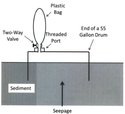
2.3.5 Lee-Type Seepage Meters
A Lee-type seepage meter consists of the end of a 55 gallon drum with a plastic bag fixed to it via a two-way valve, as shown in Fig. 2. The drum is planted in the sediment on the ocean floor with a known amount of water in the plastic bag.
Water surface Plastic
/ Bag
Seepage
Figure 2: A sketch of a Lee-type seepage meter that directly measures flow through the
sediment in either direction. Modified from Lee (1977).
At various time intervals, the volume of the plastic bag is measured. Originally, this was done by removing and replacing the plastic bags. Now modem Lee-type meters have sensors that can detect water flow through the valve. Starting with an initial volume of water in the bag allows flow to be measured weather it flows through the sediment into the meter or from the meter out through the sediment. Knowing the composition of the water that started in the bag allows for calculation of composition of water that seeps into the bag through mass balance of salt or other geochemical tracers.
Lee-type meters provide an accurate, direct measurement of SGD and can be left in place to observe temporal discharge trends. They do, however, take a great deal of time and effort to install, and provide extremely localized data. A large number of them would be required to measure spatial variations. They also cannot be installed in karstic or rocky formations, where point source discharge is expected.
2.3.6 Other Observable Signs of SGD
The first recorded instances of SGD were seen by sailors as early as the first century A.D. (Burnett 2003). The signs included patches of differently colored water, bubbles at the surface, and tasting freshwater in the ocean. Other signs include areas with abnormally dense fish populations. Dr. Matthew Charette advised the author that, from his experience, the first step in
looking for SGD in a new area is asking the local fishermen if they knew of any of these phenomena or other localized abnormalities.
2.4 Submarine Groundwater Discharge in Cyprus
A small, semi-arid island in the eastern Mediterranean, Cyprus has a history of water
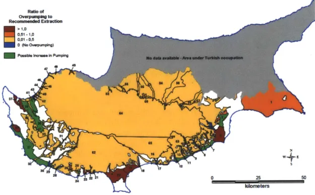
shortages. The last several decades have been particularly dry, with the average rainfall dropping from 515 mm/yr over the time period from 1961 - 2000, to 435 mm/yr from 1971 - 2000 (Georgiou 2002). For a long time, the majority of the country's aquifers were over-pumped beyond sustainable rates (see Fig. 3). This has resulted in salt water intrusion in coastal aquifers and depletion of inland aquifers.
Figure 3: Map of Cyprus showing aquifers and the ratio of over-pumping to
recommended extraction. The aquifers colored red are pumped at a rate more than twice the recommended sustainable extraction. Reproduced from Georgiou (2002).
Because of the frequent water deficits, the Water Development Department (WDD) carried out the Re-Assessment of the Water Resources and Demand of the Island of Cyprus project in 2002 with the help of the Food and Agriculture Organization of the United Nations (FAO). The majority of the information about groundwater in Cyprus comes from this project. It should be noted that almost all of the information is regarding the portion of the island under government control; very little data is available about the part of Cyprus occupied by Turkey.
The total water demand' for Cyprus was estimated as 265.9 mcm/yr (ie million cubic meters per year) in 2001 (Savvides 2001). This value has most likely increased since then due to population growth. An assessment of groundwater resources approximated that the total recommended sustainable extraction for all of the aquifers in government-controlled Cyprus is on the order of 81 mcm/yr (Georgiou 2002). In the past decade the Cypriot government has been forced to turn to desalination plants to make up the difference.
As of the end of 2010, desalination plants produced 65.7 mcm/yr (WDD 2010). Thanks to these plants and higher than average rainfall in the past couple years, the water deficit has shrunk. However desalination plants are not a perfect solution; they require 4.5 kWh of energy to produce a cubic meter of potable water which costs approximately E 1.01 per cubic meter, which is variable and highly dependent on oil prices (Manoli 2010). Additionally this water comes at the price of greenhouse gas emissions and the as of yet unknown long-term consequences of increased localized salinity due to brine rejection from these plants.
All studies of groundwater resources in Cyprus thus far have been based on mathematical
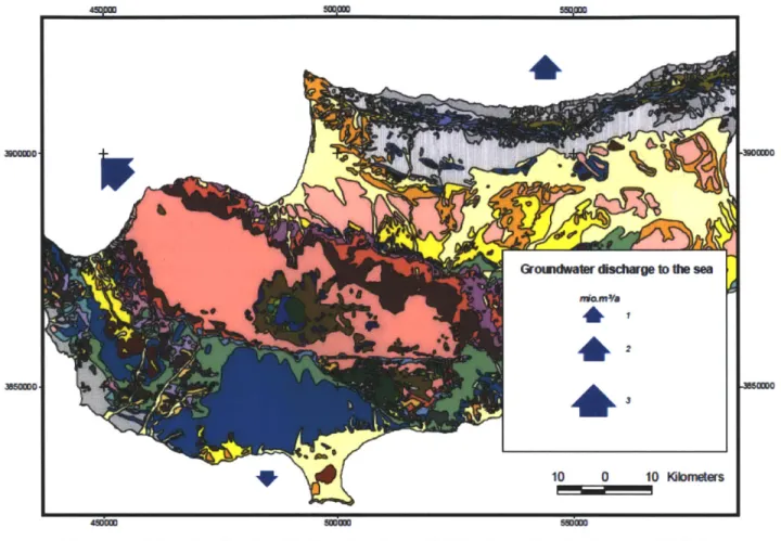
equations and models based on some measured data and a good deal of estimation and experience on the part of the investigators. Approximations of SGD have been made using Darcy's Law (1) and groundwater flow models applied to individual aquifers, and vary greatly. The assessment of groundwater resources from 2002, which seems to be the most reliable and transparent regarding methods, estimates that 24.6 mcm/yr is discharged into the sea (Georgiou 2002). A re-evaluation of groundwater resources performed in 2004 gives several different approximations of sea losses, each obtained using slightly different models and input parameters. The report first states that 72.7 mcm/yr is lost to the sea via both SGD and surface flow (i.e. rivers and streams). Later in the report, the total value of sea losses is calculated as 217.2 mcm/yr, with no explanation as to the discrepancy. Estimates in different sections of the report give the amount of water lost to the sea as surface flow as 18.8 mcm/yr and the amount lost as groundwater discharge as 6 mcm/yr (Udluft 2004). Fig. 4 shows a map of Cyprus from this report with arrows representing likely locations of SGD. It is clear from the range of these values that further work is needed for more precise approximations of SGD.
Water demand is defined in this case as "the normal water requirement for any sector (Agriculture, Domestic, Industry, etc.) expressed either as total amount or per unit area, per capita consumption etc. It is the necessary water demand to cover the needs of a sector without shortage" (Savvides 2001). Water demand is usually greater than water use, which varies year to year based on water availability.
Figure 4: Map showing localized estimations of SGD from the GRC report (Udluft
2004). These estimates come from Darcy's Law. Other estimates based on groundwater flow models within the same report suggested that up to 217.2 mcm/yr (million cubic meters per year) were discharged to the sea across the country. Reproduced from Udluft (2004).
If a point source of SGD were found near Cyprus that was large enough to be tapped or
contained, it could potentially reduce the burden on the desalination plants, making the investigation for SGD worthwhile. Even if this were not the case, however, any information that could be used to produce a more accurate depiction of outflow to the sea in Cyprus would be beneficial from a water policy and management perspective.
2.5 Proposed Procedure for Cyprus
Because no experimental work had been done in Cyprus to locate or quantify SGD prior to this investigation, aerial TIR was selected as the first method to search for any indication of groundwater discharge because it could quickly cover a large area. An infrared camera owned by the Cyprus Institute was to be used for the study (further details can be found in Sections 4.1.2.1 -4.1.2.2). A great deal of thought was put in to what type of vehicle to which to mount the camera.
Vehicles considered included a manned, fixed winged aircraft, several models of fixed-winged UAVs (unmanned aerial vehicles) and RC (remote control) aircrafts, a small quadrotor
(UAV and/or RC), an RC blimp, and a weather balloon tethered to and towed by a boat. The
UAVs and RC aircrafts that were reasonable to make operational in the time frame of this project did not have a long enough battery life for the planned mission and were too small to withstand the wind speeds that they would face over the Mediterranean Sea. A tethered weather balloon was a very tempting option, as it would allow the investigators to obtain data without the need for a pilot and co-pilot. In the end, however, it was determined that the speed obtainable with a manned aircraft made it a more cost-effective solution than renting a boat to which to tether the balloon. More data could be obtained for a given price with the manned aircraft than with the balloon towed by a boat.
After analyzing the data obtained from TIR, salinity would be tested in situ with a Conductivity-Temperature-Depth (CTD) sensor in any areas that showed anomalous temperatures. Using salinity as a tracer rather than any other chemical ensured that it would be applicable across the entire island, whereas tracers naturally occurring in groundwater in one part of the island may not necessarily be prevalent in another part.
For this first phase of the SGD project, the proposed procedure here described would be carried out only over a small portion of the Cypriot coastline. Through this experience, it would be improved upon. The revised procedure would then be tested and refined once more to make final changes before a full-scale investigation of SGD in the coastal waters of the island was launched in the spring, when rainfall, and thus SGD, is highest. With this end goal in mind, the procedure was designed to be efficient and effective enough to eventually be carried out across the whole coastline, over the range from 0-10 km from shore to cover nearshore and embayment
scales of SGD.
Prior to carrying out the procedure in Cyprus, a location was found in New England to test certain aspects of the protocol and develop data processing methods.
3. Testing in Quonochontaug Pond, RI
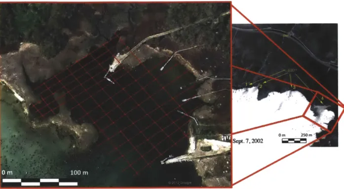
Quonochontaug Pond is one of several salt water ponds along the coast of Rhode Island. It covers an area of 3.02 km2 with an average depth of 1.8 m and average salinity of 29 ppt. It is connected to the Atlantic Ocean via a large causeway and thus Prior work done in the area by Dr. Charette, from Woods Hole Oceanographic Institute, provided the TIR shown in Fig. 5, which shows areas of potential SGD.
Figure 5: Aerial thermal image of northeast coast of Quonochontaug Pond, RI showing
four locations with evidence of submarine groundwater discharge. Location 4 on the map was selected to test the salinity profiling procedure. Infrared image provided courtesy of Dr. Matthew Charette, through research made possible by the financial support of the Woods Hole Oceanographic Institution's Coastal Ocean Institute and the Cove Point Foundation. Google Earth screenshot: 0 2012 Google 0 2012 Europa Technologies C 2012 TerraMetrics.
Quonochontaug Pond (specifically location 4 shown in Fig. 5) was selected as a location to perform a test run of the salinity profiling procedure prior to traveling to Cyprus.
3.1 Salinity Profiling
3.1.1 Conductivity, Temperature and Depth Sensor
The YSI CastAwayTM-CTD (S/N llB100023YSI Incorporated, Yellow Springs, OH) was used to map the salinity in the northeast corner of the pond. The YSI CastAwayTM-CTD is powered by two AA batteries, weighs approximately 1 lb., and records data at a sampling rate of
5 Hz. It is equipped with GPS which it uses to record the precise location and time at the start and finish of each measurement. Every data point is linked to the corresponding locations and times. The CTD comes pre-calibrated from the factory. The manufacturer recommends returning the instrument to the factory yearly for re-calibration.
Three CTD-fixed sensors measure water conductivity, temperature, and pressure (Fig. 6). Depth, salinity, specific conductance, and sound speed are derived from these properties. Only salinity and depth are employed in the scope of this study
LCD
' Screen
Pressure
3ensor Port ContainingFlow Cell
Conductivity
- Electrodes
and Temperature
Sensor
Figure 6: YSI CastAwayTM -CTD showing sensor and electrode locations
Six electrodes within the CTD's flow-through channel are used to measure resistance; two electrodes generate an electrical current while the other four electrodes measure resistivity. Only two electrodes are necessary to measure resistance; the additional electrodes improve accuracy and reduce the risk of calibration errors. From this measured resistivity, the conductivity of the water in the cell is calculated with the equation:
(6)
C = 1
where C is the conductivity, I is the distance between the electrodes, R is the measured resistivity, and A is the cross-sectional area of the flow-through channel. A thermistor, or a material with a temperature-dependent resistance, provides the temperature data.
Conductivity of water is dependent on temperature, the concentration of ions present and (to a lesser extent) pressure. The majority of ions in water come from salt. Thus salinity can be derived from conductivity, temperature and pressure. This relationship is given by the Equation of State of Seawater, or EOS-80. The EOS-80 conversion from conductivity to water is a complicated series of four numerically developed (as opposed to analytically developed) equations intended to be solved by a computer. Details of the computation, along with a discussion of the practical salinity scale, can be found in the UNESCO technical paper, "Algorithms for Computation of Fundamental Properties of Seawater" (Fofonoff 1983). This computation is performed within the CTD.
Depth is not measured directly by the CTD, but rather a sensor measures the gauge hydrostatic pressure, which is then used to calculate depth. The CTD uses the temperature and salinity measurement to obtain water density and the latitude and altitude measured by the internal GPS receiver to find the local acceleration due to gravity. Together these data allow for the calculation of depth.
The CTD can take two types of measurements: casts and point measurements. In either case, a rope is tied securely to a carabiner attached to one end of the instrument and to a fixed object on the other end in case the rope were to slip. The rope can either be held in an investigator's hands or lowered with a winch.
During a cast, the sensor is lowered to just below the surface of the water, where it is held stationary for 5-10 seconds before it is allowed to free fall to the deepest point of measurement. The instrument is then immediately raised at a recommended steady rate of approximately 1 meter per second. While moving through the water, the CTD takes a series of measurements at a sample rate of 5 Hz. The result is a profile of the measured water properties with respect to depth.
For a point measurement, the CTD is lowered to the desired position and moved either up and down or back and forth to keep water flowing through the measurement cell for approximately 5 seconds. All properties at that location are recorded as a single data point.
The CTD is capable of storing up to 15 MB of data, or approximately 750 typical casts. Data collected can be reviewed on an LCD screen at any time. Bluetooth technology is used to download data onto a Windows-compatible computer. Software accompanying the CTD allows for easy viewing of locations of measurements and comparison of individual casts or point measurement.
3.1.2 Determination of Measurement Locations
Before the field test date, Google Earth software was used to locate the area exhibiting signs of SGD based on the aerial thermal images. In order to systematically determine measurement locations, a grid was drawn over the area with intentionally smaller spatial resolution near the shoreline where SGD was suspected, as shown in Fig. 7. The latitude and longitude at each of the
90 intersections of the grid was found using Google Earth; a list of each of these coordinates was
SW
m, 200
100m
Figure 7: Grid was drawn over area of interest using Google Earth. Latitudinal and longitudinal coordinates of each point of intersection on the grid were recorded and used to determine measurement locations during field testing. Grid spacing was intentionally smaller near northwest section of area where submarine groundwater discharge is believed to occur based on aerial thermal image. Google Earth screenshot: C 2012 Google.
While the CTD tracks and records GPS locations for each measurement, it does not display
GPS coordinates between uses. Thus the investigator used a handheld Garmin GPSMAP 60CSx
Hiking GPS Receiver to find each of the pre-determined GPS coordinates for point measurements.
3.1.3 Point Measurements of Salinity and Temperature
Field sampling was done on June 26, 2011 between 12:08pm and 4:30pm EST with a YSI
CastawayTM - CTD from onboard a kayak. Because water in the area of interest was very shallow (ranging from approximately 0.2 m to 1.1 in), the CTD was used to obtain point measurements rather than water column profiles. The CTD is designed to take measurements while water is moving through the flow cell; thus in order to measure salinity and temperature, the CTD was slowly moved for several seconds either back and forth or up and down through the water depending on the depth of the water at that particular location.
Profiles were obtained by interpolating the measured properties between measurement positions. The MATLAB scripts required to graph these profiles along with detailed instructions of how these scripts are used are found in Appendices A-C.
3.2 Quonochontaug Pond Results and Discussion
Fig. 8 illustrates cast locations as recorded by GPS onboard the CTD and the resulting salinity profile.
I I
sairPsSS]
Figure 8: Salinity profile as measured by CTD. The black diamonds denote locations of point measurements given by GPS in CTD. Google Earth screenshot: C 2012 Google.
The majority of the measurements obtained gave salinities around 26 on the practical salinity scale (orange in Fig. 8). Salinities near the northern coast drop down to approximately 20. This corresponds with the darkest area in Fig. 5, and is likely a result of freshwater discharge. The dark blue patch on the western edge of the data collection region also corresponds to a darker area on the infrared image in Fig. 5 that appears to originate from a stream. A list of the salinity measurements are given in Appendix D.
The GPS coordinates of the intended measurement locations were brought onboard the kayak during testing with the intent of measuring temperature and salinity at evenly distributed points spanning the area of interest. It was difficult to specify a precise measurement location
due to wind moving the kayak and currents moving the CTD. Therefore, the intended locations were used as guidelines. Although time consuming to find in the kayak, the printed GPS coordinates were helpful in open water to ensure that the entire area was covered. However, near the coastline or around anchored boats it was easy to navigate the kayak in a straight line using these as reference points, so measurements were taken at locations determined by the investigator on site rather than finding the GPS coordinates.
Some points at which measurements were desired were left off due to obstructions in the pond. Nests and wildlife along the shoreline prevented measurements from being taken too close to the coast. Other points were unreachable due to thick plants that had grown in since the satellite image, which was used to grid the area, was taken.
Because Quonochontaug Pond has a large breach-way directly connected to the Atlantic Ocean, it experiences high and low tides. Testing occurred between low tide, which occurred at 11:00am, and high tide, which occurred at 5:33pm. Because SGD is driven by the hydraulic gradient between groundwater and sea level, SGD rates are highest, and thus most observable, during low tide. Testing could not occur entirely at low tide due to the time-intensive process. After the entire area was measured, the north shore, where measurements were taken first, was revisited. The results did not differ significantly from the initial measurements.
4. Testing in Cyprus
Before the procedure could be tested, a location was selected based on the likelihood that
SGD would be observed and how easily the procedure could be implemented. The investigation
was limited to the southern, Greek-Cypriot side of the island due to political reasons. Based estimations of SGD in the GRC report (shown in Fig. 4), the focus was narrowed to Episkopi Bay along the southern coast and Chrysochou Bay on the northwest coast. Several local fishermen and residents of Polis and surrounding cities claimed to have seen signs of water discharge in Chrysochou Bay, including areas of unexpectedly high fish populations, water appearing to be drunk by animals at certain spots along the coast, and bubbles at the surface at low tide on calm days. Based on this combination of information, Chrysochou Bay was selected as the ideal location for testing the procedure.
By design, TIR was intended to be performed prior to salinity measurements. The results of
the aerial imaging data would determine locations of salinity testing. However, permission to fly data acquisition missions was not granted by the Cyprus Department of Civil Aviation in time to allow this. As a result, the procedure was altered to accommodate taking salinity measurements prior to aerial imaging.
4.1 Procedure
3.1.1 Salinity Measurements
The same YSI CastawayTM - CTD used in Quonochontaug Pond as discussed previously
was used in Cyprus. The primary differences were the depth of the water and the vehicle from which the CTD was used. While in Rhode Island the shallow water necessitated point measurements, in Cyprus the cast feature of the CTD was used to measure salinity over the full water column. In order to perform these casts, the CTD was attached to a motorized fishing rod via a fishing line rated for 200 lbs of force. The rod was set to lower and raise the instrument at a fixed speed of 1 m/s, as recommended by YSI. Measurements were taken from onboard an inflatable commercial fishing boat.
The boat was rented for the day along with its captain. The captain was told of the purpose of the investigation prior to being hired. He was familiar with the phenomenon of SGD and had heard of and witnessed signs of SGD in Chrysochou Bay. Three locations were visited based on his recommendation, as shown in Fig. 9.
Figure 9: Locations in Chrysochou Bay singled out by fishermen and locals as showing
signs of freshwater SGD. Signs included: goats appearing to drink water from the ocean, higher localized fish populations, and bubbles at the ocean surface on calm days. Salinity was measured at each of these locations. Google Earth screenshots: Left: C 2012 Europa Technologies, Image C 2012 DigitalGlobe, © 2012 Google, Data SIO, NOAA, US Navy,
NGA, GEBCO. Right: Image © 2012 DigitalGlobe, Data SIO, NOAA, US Navy, NGA, GEBCO.
At each spot sample casts were performed to determine whether salinity measurements were anomalous in that area, using the LCD screen on the CTD to check the data on site. The number of sample casts ranged from two to fifteen depending on the size of the area. If low salinities were observed, salinity measurements were repeated throughout the entire area to obtain adequate data to produce a salinity profile. The data recorded during each cast was used to inform the spacing between subsequent measurements; if a low salinity was measured, the distribution of cast locations in the immediate vicinity of that cast was denser than if the measured salinity was high.
4.1.2 Aerial Imaging
4.1.2.1 Infrared Video Camera
The infrared camera used to obtain the TIR video in Cyprus was the FUR Photon 640, equipped with a 60mm lens. The Photon 640 is designed for minimal payload for aerial applications. The sensor is a 640 x 512 uncooled vanadium oxide microbolometer array. It has a spectral band of 7.5 to 13.5 pim and a noise equivalent differential temperature - which is representative of the minimum detectable temperature difference - of 50 mK. This is more sensitive than most cameras used for aerial TIR studies of SGD, which are commonly 100 mK (Mulligan 2005, Duarte 2006, Johnson 2008). It should be noted however that while the sensor is capable of detecting these temperatures, the 8-bit analog video output significantly limits the temperature differences shown by the final data. The video produced is National Television System Committee (NTSC) analog video, which has a frame rate of 30 Hz. The lens used with the camera has a focal length of 60 mm and a field of view of 150 by 110. The instantaneous field of view is 0.416 milliradians. Together, these specifications can be used to calculate the dimensions of the area captured by the camera in a single frame and in a single pixel within that frame as shown in Fig. 10.
VFOV
Figure 10: The horizontal and vertical length (H and V respectively) of the area captured by the camera within a single frame and within a single pixel can be calculated using the
horizontal and vertical, and instantaneous fields of view (HFOV, VFOV and IFOV) of the lens as well as the distance of the lens from the image plane (a).
From this image, it is clear that the horizontal length, H, area captured in a frame are given by
H = 2a * tan (HFOV)
V = 2a * tan (VFOV)
and
and the vertical length, V, of the
(7)
(8)
where a is the distance between the camera and the target (in this case the altitude of the plane and HFOV and VFOV are the angular horizontal and vertical (respectively) fields of view of the lens. The small angle approximation gives that the length of either side of the area depicted by any individual pixel, p, is
p = a* IFOV (9)
where IFOV is the angular instantaneous field of view of the lens. Given a desired spatial resolution, Eqn. (9) can be used to calculate the necessary altitude. For example, if a resolution
of 0.5 m per pixel is desired, Eqn. (9) is solved for a using the camera's IFOV of 0.416 milliradians, giving
0.5 m
a-= = 1202 m
0.416 * 10-3
Thus if the camera is 1202 m away from the subject being recorded (i.e. the plane is flown at an altitude of 1202 m in the case of aerial imaging of the ocean surface), each pixel will represent a square with sides of length 0.5 m. The entire area shown in a frame can be found by
applying Eqn. (7) and (8), which give
H 2 * 1202 m * tan ( ) = 316.5 m
and V= 2 * 1202 m * tan ) = 231.5 m
In the case of surveying a large area using the infrared camera such as was done within this study, Eqn. (7) can be used to calculate the width covered in a single pass, and therefore the allowable distance between consecutive parallel passes to achieve desired overlap of images, ensuring full coverage of the area under investigation.
4.1.2.2 Cloud Cap Technology Gimbal
The FLIR Photon 640 infrared camera was used as an integrated component along with a visual camera in a Cloud Cap Technology Tase200 Gimbal, shown in Fig. 11. For the purposes of this investigation, only the infrared camera was used to collect data. All user interfacing was done with the Cloud Cap gimbal and associated software rather than directly with the FLIR camera. The visual camera was occasionally used to assess camera mount vibration or to orient the gimbal in situations where infrared video was inadequate.
Figure 11: A Cloud Cap Technology TASE200 Gimbal, shown here, was used to obtain
thermal images. Image reproduced from CloudCapTech.com
When in use, the camera is connected to a laptop on which ViewPoint, the Cloud Cap software, is running (see Fig. 12). Through ViewPoint, the investigator is able to watch the video feed in real time, adjust camera orientation, monitor GPS and other data, and change certain settings on the camera. After recording the data, ViewPoint can also be used to export the video recorded and the GPS data associated with specified frames to a form usable by other programs.
'7 -7 77.
I. IMI.IUI*1W11
Figure 12: Screen shot of ViewPoint software during camera operations. Displays, from
top left, status lights, playback controls, streaming video, gimbal telemetry data, and image footprint on map.
The output from the IR camera is video made from a series of 640x480 8-bit grayscale images. This means that based on the amount of incident energy on the camera's sensor, every pixel within a frame is assigned a value from 0 to 255. This value is called the pixel intensity. A pixel with an intensity of 0 is shown as black, 255 is shown as white, and all others fall on the spectrum from black to white.
4.1.2.3 Relating Infrared Images to Temperature Differences
As discussed in Section 2.3.2.1, the absolute temperature is difficult to calculate from TIR and is not necessary in finding anomalous areas indicative of SGD; however, if a relationship were known between the image output from the IR camera and the temperature of the subject of the image, it would be possible to determine a difference in temperature between two areas in a frame by measuring the difference in pixel intensities.
In order to quantify the relative difference in temperature between different pixel intensities in the resulting image, a glass of ice water was recorded using the gimbal in the lab as it warmed to room temperature (see Fig. 13).
Gimbal Mounted on Ceiling Connected to Laptop Running View Point Software Glass of Water Connected to Fluke Digital Multimeter emperature Probe
The temperature of the water was measured using a Fluke temperature integrated digital multimeter probe at time intervals determined by the rate of change of the temperature of the water. The time of measurement was also recorded and used to correlate the temperature measurement to a given frame. The frame was then exported as a snapshot from the ViewPoint software and ImageJ was used to measure the mode pixel intensity within the cup. The mode was used rather than the mean because there was a clear radial gradient in pixel intensity, which caused a large variation in mean based on the selection area. Because the camera adjusted brightness to keep the average temperature in a given frame at the middle of the grayscale spectrum, at a pixel intensity of approximately 127, the background color changed throughout the recording. To compensate for this, the average background pixel intensity was subtracted from the water pixel intensity.
Once the cup of cold water had warmed sufficiently procedure was repeated with a cup of warm water. The temperature and pixel intensity is shown in Fig. 14.
200 150 100 50 0 -50 -100 -150 -200
close to room temperature, the measured relationship between
, measurements
60 Fit Curve
Temperature [degC]
Figure 14: The relationship between temperature and pixel intensity was measured in a
lab setting. A cup of first cold water and then of hot water were recorded as they approached room temperature. The differences between the mode pixel intensities within the cup and the mean pixel intensities of the background and the temperatures of the water in the corresponding frames were measured and are shown here.
A curve fit to the data had the equation
where p is the difference between mode water pixel intensity and the mean background pixel intensity and T is the temperature of the water. The R2 value for the fit curve was 0.9982,
indicating a good fit.
The original intent of this was to determine the difference in pixel intensities that constituted a significant variation. However, time did not allow these results to be verified. For this investigation, any areas that could be identified as anomalous were considered significant. Further work should be done in the future to better understand the relationship between pixel intensity and temperature using this gimbal.
4.1.2.4 Flight Vehicle
A Cessna 172 Skyhawk was chosen as the appropriate vehicle for acquiring TIR due to its
accessibility in Cyprus and flexibility in flight mission capabilities. The aircraft was hired along with a pilot and co-pilot by the hour. The gimbal was mounted on a support beam as shown in Fig. 15.
Figure 15: The gimbal was mounted to a support beam on a Cessna 172 Skyhawk. The mount was built by one of the pilots hired to fly the plane. Vibration-dampening mounts supplied by Cloud Cap were used between the camera and the mount structure.
The gimbal mount was built by the hired pilot and consisted of a structure made of wood reinforced with woven fiberglass fabric. The structure was affixed to the beam via several cable ties. Efforts to minimize vibration included vibration-dampening compression mounts, which were supplied by Cloud Cap, between the gimbal and the mounting structure, and a layer of foam between the mount structure and the beam. The gimbal's GPS unit was cable-tied to a protruding rail on the nose of the aircraft. Any lengths of wires on the outside of the plane were taped to the side of the plane to keep them from moving during flight.
Wires from the gimbal system were run through the window to the back seat, where two investigators had a laptop computer running the ViewPoint software. A lithium ion battery onboard the aircraft supplied power to the camera. The voltage of this battery was checked often; if it were to run low, it would be substituted by a spare battery that was also onboard. An inverter
and a 12 V lead acid battery were used to power the laptop. Both of these were fixed to a wooden board which was then secured to the floor in the rear of the plane to eliminate the risk of these heavy objects causing injury should the aircraft experience turbulence or other problems.
A test flight was used prior to the data acquisition flights to ensure that all equipment
functioned properly and that the vibration of the gimbal would not impede the video feed.
4.1.2.5 Aerial Imaging Procedure
Data acquisition missions were flown on August 4th and August 5th, 2011. Because the sun tends to heat the sea surface to a uniform temperature after it has been up for more than a couple hours, both flights were scheduled to take off as early as possible from the Larnaca airport. Typically Larnaca is foggy around sunrise, so the plane took off as soon as the fog had cleared to a safe level. All data was obtained between the hours of 8:30 am and 9:15 am local time.
A flight plan that included waypoint GPS coordinates and headings was made and discussed
with the pilots prior to take off (see Fig. 16).
Figure 16: Flight path created in Google Earth. A copy of the above image and a list of
waypoint GPS coordinates were given to the pilots prior to takeoff. C 2011 Europa Technologies, Data SIO, NOAA, US Navy, NGA, GEBCO, C 2011 Google, Image
C 2011 DigitalGlobe.
The studies used to inform the design of the experimental protocol used a spatial resolution ranging from 0.2 m per pixel (Torgersen 2000) to 3 m per pixel (Duarte 2006) in aerial thermal images, with the majority of the studies falling within the 0.5 m to 1.0 m per pixel range. It was