Design of a Shock Tube for Jet Noise Research
by
John Matthew Kerwin
S.B. Aeronautics and Astronautics, Massachusetts Institute of Technology, 1994
Submitted to the Department of Aeronautics and Astronautics
in partial fulfillment of the requirements for the degree of
Master of Science
at the
MASSACHUSETTS INSTITUTE OF TECHNOLOGY
June 1996
@
Massachusetts Institute of Technology 1996. All rights reserved.
Author ...
.
. ... ..
...
Department of Aeronautics and Astronautics
April 16, 1996
/2
Certified by ...
..
.. ...'
...
... ...
Professor Ian A. Waitz
Assistant Professor of Aeronautics and Astronautics
Thesis Supervisor
Accepted by ... .. . .
;Am.i !l .. \
/...
-.. -. --ProfessorHarold Y. Wachman...
...
Chairman, Department Graduate Committee
Aero
M OASFSACHUSET-S INS;i i OF TECHNOLOGY
Design of a Shock Tube for Jet Noise Research
by
John Matthew Kerwin
Submitted to the Department of Aeronautics and Astronautics on April 16, 1996, in partial fulfillment of the
requirements for the degree of Master of Science
Abstract
This thesis describes the design of a shock tube for the study of supersonic free jets. The primary purpose of the facility will be to study noise suppressor nozzles for application on supersonic civil transport aircraft. The shock tube has many strengths; it is mechanically simple, versatile, has low operating costs, and can generate acoustic and fluid dynamic data that is comparable to that of steady state facilities.
A reflection-type shock tube was designed to produce a reservoir of fluid at total tem-peratures and pressures analogous to those at the exit of a gas turbine engine. This fluid will be exhausted through a nozzle, generating a turbulent jet inside an anechoic test cell. Using air as the test gas, jet total temperatures up to 1750 K and total pressures up to 38
atm can be achieved. In addition, the shock heating creates highly uniform total
temper-ature and pressure profiles at the nozzle inlet, eliminating the core noise often present in steady-state, vitiated air facilities. Lastly, the short duration of the test allows for relatively inexpensive stereo-lithography nozzles to be tested at realistic flow conditions. Fluid dy-namic and acoustic measurements including thrust, Mie scattering to determine mixedness, and far-field noise will be taken in the facility.
An analysis is presented of the shock tube and fluid jet, and a detailed mechanical de-sign of the facility is included. The optimum shock tube geometry was established using an ideal one-dimensional gas dynamic model with corrections to account for the growth of an unsteady boundary-layer. The nozzle and jet starting processes were investigated to estimate the duration of the quasi-steady, fully-developed jet. Requirements for noise mea-surements are discussed, including frequency scaling, high frequency measurement limits, uncertainties in power spectral analysis, and required sampling times.
Two shock tube configurations are presented: (1) an 8" diameter, 38' long, vertical shock tube with a 16' x 19' test cell and (2) a 12" diameter, 60' long, horizontal shock tube with a 19' x 26' test cell. The 12" facility will be constructed. Using this facility 18 ms duration tests can be performed on a 5.2" exit diameter noise suppressor nozzle (roughly 1/1 2th of full scale). Frequencies up to 80 kHz (corresponding to 6.7 kHz full scale) can be measured, and it is expected that noise power spectrum measurements within ±2 dB can be obtained with 3 shock tube runs for full scale frequencies above 500 Hz .
Thesis Supervisor: Professor Ian A. Waitz
Acknowledgments
The completion of this thesis would have been impossible without the advice, assistance and friendship of a number of people. Foremost, I would like to thank Prof. Ian A. Waitz for providing me with countless opportunities throughout my stay at MIT and for his guidance during this project. I am also deeply indebted to Dr. Gerry Guenette for his enthusiasm and mechanical inspirations, and to Prof. Edward Greitzer for his many insights into the project.
There are many others I would like to thank:
To Prof. Uno Ingard, Mr. Chet Killam, Prof. Mohammad Durali, Dr. David
Davidson, Dr. Mike Miller, Mr. Daniel Yukon and Dr. Terry Parker for all their
help and expertise along the way.
To Dr. Choon Tan for friendly advice and funding our caffeine addiction.
To my officemates Greg Stanislaw, Dave Tew, Luc Frechette and "F-as-in-Frank" Fouzi Al-Essa for their friendship, humor, advice, sarcasm, raillery, and general tomfool-ery.
To my Unified comrades, Sonia, Julian, and Mike for having the tenacity to still be here, and to Christine, Jun, and Larry for having the good sense to get away.
To Willy for five years of wit, friendship, adventures, and all-nighters.
A special thanks to Kaesmene, a close friend, poet, and editor for helping me with my prose, and to Elliott, a long time friend, for being there through it all.
To my sister for her free psychoanalysis and counseling.
And, most of all, to my parents for their loving support; this thesis is dedicated to them.
Support for this project was provided by NASA Langley, under contract NAG-1-1511 and supervision of John. M. Seiner. This support is gratefully acknowledged.
Contents
Nomenclature
11
1 Introduction
14
1.1 Background ... ... 14 1.2 M otivation . . . 15 1.3 Facility Objectives ... 17 1.4 Facility Overview ... ... .. 181.4.1 8" Diameter Vertical Shock Tube . ... . 18
1.4.2 12" Diameter Horizontal Shock Tube . ... 19
1.5 Thesis Overview ... 22
2 Shock Tube Gas-Dynamic Design
24
2.1 The Wave System in a Simple Shock Tube . ... 242.1.1 The Shock Tube Equation ... 26
2.1.2 Shock Reflection ... 27
2.1.3 Interface Tailoring ... 30
2.1.4 Interaction of a Shock Wave overtaking an Expansion . ... 30
2.2 Boundary Layer Effects ... 31
2.2.1 Boundary Layer Model ... 32
2.2.2 Shock Attenuation ... 34
2.2.3 Free Stream Acceleration ... 35
2.2.4 Influence of Boundary Layer on Time-Distance History . ... 35
2.2.5 Reflected Shock-Boundary Layer Interaction . ... 37
2.3 Duration of Constant Conditions in Reservoir . ... 39
2.3.2 Test Gas Exhaustion Limited Test Times . . . 2.4 Gas-Dynamic Performance and Design . . . . 2.4.1 Establishing Gas-Dynamic Performance Curves 2.4.2 Setting Tube Geometry to Optimize Test Time 2.4.3 Shock Tube Loading . . . . 2.5 Gas-Dynamic Design Summary . . . .
3 Generation and Acoustics of the Scaled Jet 3.1 Jet Noise Generation and Scaling . . . .
3.1.1 The HSCT Nozzle ...
3.1.2 Noise Generation Mechanisms . . . . 3.1.3 Effective Source Distribution . . . . 3.1.4 Effect of Flight Condition . . . .... 3.1.5 Frequency Scaling ...
3.2 Acoustic Measurement Constraints . . . . 3.2.1 Far-Field Distance ...
3.2.2 High Frequency Measurements . . . . 3.2.3 Directivity Angles ...
3.2.4 Acoustic Sampling Time . . . . 3.3 Jet Start-up time ...
3.3.1 Jet Development Model . . . . 3.3.2 Nozzle Starting Model ...
3.4 Room Acoustics ...
3.4.1 Anechoic Treatment of Room . . . . 3.4.2 Start-up noise ...
3.5 Summary of Facility Performance for Various Nozz] 3.5.1 8" Vertical Shock Tube Facility . . . ...
3.5.2 12" Horizontal Shock Tube Facility . . . . . 3.5.3 Facility Performance Trends . . . .
53 . . . . . 55 . . . . 55 . . . . . 56 . . . . . 57 . . . . . 57 . . . . 58 . . . . . 59 . . . . 59 . . . . . 59 . . . . 60 . . . . . 63 . . . . 67 . . . . . 67 . . . . 68 . . . . 69
. . . .
.
69
.. . .. .. .. . .. ..
69
le Configurations . . . . 70 4 Mechanical Design 4.1 The Driver and Driven Sections ... ... 4.2 The Primary Diaphragm Assembly . . . . 7777
81 . . . . . 4 1 . . . . . 44 . . . . . 44 . . . . . 484.2.1 Single Diaphragm Method ... 4.2.2 Double Diaphragm Method ... 4.2.3 The Knife Blades ...
4.2.4 Cross Section & Transition ... 4.2.5 Diaphragm Retention ...
4.3 Secondary Diaphragm/Nozzle Assembly ... 4.3.1 Secondary Diaphragm ...
4.4 Mechanical Changes for 12" Shock Tube Facility
5 Closure
5.1 Sum m ary . . . . 5.2 Conclusion . . . . A Gas Dynamic Model
A.1 Fundamental Gas Dynamic Equations . . . . A.2 Derivation of the Shock Tube Model . . . . B Boundary Layer Model
C Jet Starting Model D Mechanical Drawings . . . . 82 . . . . . 82 . . . . 84 . . . . 86 . . . . 87 . . . . . 88 . . . . 88 . . . . . 90 92 92 94 98 98 100 109 114 116
List of Figures
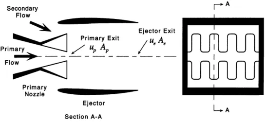
1-1 Section and rear view of a typical mixer-ejector nozzle for jet noise
suppres-sion, adapted from Lord et al. [16] ... .... .. 15
1-2 Perspective and side view of a typical lobed mixer, adapted from Presz et al. [29] . . . . 16
1-3 Facility overview of the 8" vertical shock tube. . ... 20
1-4 Test cell overview of the 8" vertical shock tube ... . . . . .. .. . 21
1-5 Test cell for the proposed 12" horizontal shock tube . . ... . 22
2-1 Schematic of wave system in shock tube . ... . 25
2-2 Time-distance history of wave system in shock tube . ... 26
2-3 Incomplete shock reflection due to massflow through nozzle. Typical nozzle area ratios will range from A*/At = 0.05 to 0.20. M, = 2.28 ... . . 29
2-4 Effect of boundary layer growth on shock tube flows. ... 31
2-5 Boundary layer approximated as steady flow over a semi-infinite flat plate through change of reference frame ... .... 32
2-6 Distance between shock and turbulent boundary layer transition point as a function of shock Mach number, Ms. Circle denotes typical HSCT operating point, p5/Po = 3.7, T5/To = 3.0. Ret = 4 x 10⁶. ... 33
2-7 Boundary layer parameters in driven section for 8" and 12" shock tube facil-ities; M, = 2.28, pi = 0.15 atm ... 34
2-8 Variation in free stream velocity due to boundary-layer growth behind the shock for the 8" and 12" shock tubes; Ms = 2.28, pl = 0.15 atm. ... 36
2-9 Illustration of time-distance histories in real and ideal shock tubes used to generate equivalent reservoir conditions . ... ... . . . . . 37
2-10 Shock Bifurcation Structure for Re < 900, 000. Figure adapted from Mark [18] . . . 37 2-11 Reynolds number at point of shock-interface interaction. ... . . 38 2-12 Expansion wave limited test times . ... . . .. .. . . 40 2-13 Expansion limited tests time per unit shock tube length (ms/f t) as a function
of reservoir temperature ratio, T5/Ti. r1 is the test time limited by reflection
from the interface, T2 the test time limited by the secondary expansion, and T3 the test time limited by the primary expansion (see Figure 2-12). ldn/lst = 0.46. 42 2-14 Expansion limited test times per unit shock tube length (ms/ft) for various
size driven sections, ldn/lst. texp = min(T2, T3). Circles indicate the optimum operating point for each geometry, i.e. the maximum possible test time per unit length for a given reservoir temperature. ... . . . . 43 2-15 Ideal time to exhaust test gas, texg/lst, for various A*/Ast. Dotted line refers
to reflected expansion limited test time. ldn/lst = 0.46 ... 45 2-16 Reservoir pressure and temperature rise as a function of incident shock Mach
number. Air is used as driven gas. ... 46
2-17 Driver composition required to satisfy tailored interface condition. %He by
mass given for He + Ar driver. ... 48
2-18 Diaphragm pressure ratio required to generate a Mach Ms shock for different
shock attenuations ... 49
2-19 Axial loading on floor mounts for a M = 3 nozzle with Ts/T1 = 3 and 10%
loss in shock Mach number. ... 51
3-1 Section and rear view of a typical mixer-ejector nozzle for jet noise
suppres-sion, adapted from Lord et al. [16] ... 56
3-2 Mixer-ejector jet noise generation mechanisms ... 57
3-3 Jet noise effective source distribution at low Mach numbers for constant
Strouhal number. Source Lilley [15] ... 58
3-4 Microphone orientation schematic for the 8" vertical shock tube. ... . 61 3-5 Measurable directivity angle range as a function of nozzle height for 8" shock
tube facility. At height (a), Hn = 13.75" and 0 = 890 to 1570. At height
3-6 Variations of the chi-square variable about its mean, SIE(S), as a function
of the number of degrees of freedom, k. The solid line bounds 80% of the
realizations, and the dotted line 90%...
3-7 Schematic of jet starting parameters .
. . . .
3-8 Non-dimensional jet starting time as a function of Ijet/De. Circle refers to
required length for HSCT experiments, Ijet/De, 7 . . . ...
3-9 "Start-up" noise associated with starting of the nozzle. (a) massflow through
nozzle as a function of time. (b) Frequency content of the start-up noise. . .
4-1
4-2
4-3
4-44-5
4-6
4-74-8
Driver Section Schematics . . . .
Driven Section Schematics . . . .
Instrumentation port schematic .
. . . .
Schematic of the primary diaphragm assembly.
Cruciform knife blade schematic .
. . . .
Exploded view of knife blade assembly. . . . . .
Primary diaphragm assembly cross section. . .
Driven section end-plate schematic . . . .
A-1 Change of reference used to simplify analysis of moving shocks ...
A-2 Time-Distance History of Wave System in Shock Tube ...
..
A-3 Primary Expansion Fan and Characteristics . ...
. . . .
.
78
. . . .
.
78
. . . .
.
81
. . . .
.
83
. . . .
.
85
. . . .
.
86
. . . .
.
88
. . . .
.
89
99
101
105
List of Tables
2.1 Summary of shock tube parameters for the 8" vertical shock tube. It = 38',
Idn/lst = 0.46... 51 2.2 Summary of shock tube parameters for the 12" horizontal shock tube. It =
60', ldn/lst = 0.46 ... 52
3.1 Approximate dimensions of full, 1/16th, and 1/2 7th scale HSCT nozzles . . 56 3.2 Maximum measurable full scale frequencies for various nozzle scales and
scaled frequency measurement limits... . . . .. .. . . 60 3.3 Summary of test time requirements for the jet noise experiments. Required
test times, T, are presented as functions of the variability (SIE(S)),
confi-dence, and bandwidth (Af) ...
65
3.4 Approximate nozzle flow-through and start-up times. The nozzle was as-sumed to be started at tstart = 3(tp + te) where tp is the residence time for
fluid in the primary nozzle and te for the ejector. . ... 68 3.5 Summary of test times and acoustic measurement ranges for the 8" vertical
shock tube facility.
t
The test gas exhaustion times are upper limits (see Chapter 2) and do no account for various test gas contamination mechanisms. Actual test times in these cases may be substantially less. . ... 71 3.6 Summary of test times and acoustic measurement ranges for the 12"Nomenclature
Roman
A cross sectional area
D diameter
Ec Ecardt number
K kinematic momentum, - 2r
fo
u
2ydyM Mach number
NPR primary nozzle pressure ratio, pt/po
Pr Prandtl number
Re Reynolds number
Ret transition Reynolds number
Sr Strouhal number = fUe
T static temperature
Tr adiabatic recovery temperature
Tt total temperature
a local speed of sound
cs shock speed
c- negative expansion characteristic
c+ positive expansion characteristic
f
frequency
hn height of nozzle above test cell floor
1 length
ljet jet length
Ipc jet potential core length
p static pressure
Pt total pressure
r distance from nozzle exit
Rmic distance to microphones
u velocity (laboratory frame)
v velocity (shock stationary frame)
x axial distance
Greek
XHe mass fraction of helium in driver gas
7 ratio of specific heats
p density
A viscosity
6 boundary layer thickness
6* boundary layer displacement thickness
Co virtual kinematic visconsity, (0.0161)/-K
Tx wall shear force
T1 arrival time of disturbance from shock-interface interaction
T2 arrival time of secondary expansion
T3 arrival time of primary expansion
Texp test time limited by reflected expansion waves
Texg test time limited by exhaustion of test gas Tjet jet starting time
Tnozzle nozzle starting time
0 boundary layer momentum thickness
4
directivity angle, measured from upstream jet axisv kinematic viscosity
Subscripts
dn
driven section
dr
driver section
c
jet centerline velocity
e
ejector exit
o
conditions immediately behind shock
p
primary stream
r
reflected shock
s
secondary stream
s
incident shock
st
shock tube
t
total or stagnation quantity
w
wall
0
ambient conditions
1 - 9
conditions in shock tube, see figure 2-2
Superscripts
primary nozzle throat
Sdenotes
shock relative frame
Miscellaneous
Chapter 1
Introduction
1.1
Background
Recently there has been a renewed interest in developing a supersonic commercial transport for trans-Pacific operations. Before a concerted design effort can be undertaken, however, it must be established whether or not such an aircraft would be environmentally viable. One of the primary environmental concerns is noise pollution in communities near airports. The current supersonic transport, the Concorde, fails to meet the FAR 36 Stage III noise regulations, and it receives a special exemption in order to operate at U.S. airports. The next generation of high speed civil transports (HSCTs) will be required to meet these regulations if they are to operate as frequently as their subsonic counterparts.
The dominant noise source at take-off and landing is the high speed exhaust jet from the engines. A significant reduction in jet velocity during this phase of operation has been widely accepted as the only promising way to meet noise goals. Current efforts to develop such a technology have focused on acoustically lined mixer-ejector nozzles similar to that shown in Figure 1-1. These nozzles use deployable chutes to mix ambient air with engine exhaust inside an acoustically treated duct. This reduces the jet exit velocity and, correspondingly, the turbulent intensity of the free jet and the associated noise. Thrust loss and weight are critical parameters for the nozzle design. To be a viable concept, a noise reduction of at least 3 EPNdB per percent thrust loss will be required, while at the same time adding less than 20% to the engine weight. It is essential, therefore, to mix the streams as rapidly as possible to reduce the required duct length, and to perform the mixing with minimal losses. Recent research has shown that a passive, lobed mixing device can be used to rapidly
Secondary Flow Ejector Exit Primary Exit /U Ae Primary A
1=1160p
-- - __ '
--
_
P_
--
Flow Primary Nozzle Ejector Section A-AFigure 1-1: Section and rear view of a typical mixer-ejector nozzle for jet noise suppression, adapted from Lord et al. [16]
mix co-flowing streams with relatively low losses [6][16]. A schematic of a lobed mixer is shown in Figure 1-2. There are two distinct flow features responsible for this rapid mixing. First, there is a larger initial interfacial mixing area between the two streams due to the convoluted trailing edge. Second, the presence of counter-rotating streamwise vortices on the interface between the two streams stretch the interface. This provides both additional mixing area and increased flow property gradients which are the driving potential for the mixing. [5]
To date, the HSCT mixer/ejectors have fallen short of the noise reduction goals. The design efforts, however, have relied largely on empirical methods. A greater emphasis on physically-based understanding of noise suppressor performance could provide a road map for optimizing designs. This is the goal of research being conducted at the Aero-Environmental Research Laboratory at MIT. Experimental and computational tests have provided insights into the detailed fluid mechanics of noise suppressor nozzles [35][36][13] and allowed for the creation of models of gross fluid mechanical behavior [6]. Currently, a system-level model is being developed to provide a physically-based noise suppressor design tool. One critical component of an effective noise suppressor system model which does not currently exist is a simplified acoustic sub-model.
1.2
Motivation
In order to establish links between the dominant flow structures and acoustic radiation of hot supersonic jets and to enable the development of simplified acoustic models, carefully
U1
___D_
(XJ
t
U - -- - h SIDE VIEW
Figure 1-2: Perspective and side view of a typical lobed mixer, adapted from Presz et al. [29]
controlled experiments need to be conducted. An ideal facility for these tests is an acous-tic shock tube. Over certain operating ranges a shock tube can be used to produce fluid mechanic and acoustic data which matches that obtained in steady-state facilities. Further-more, the facility can provide an economical, rapid prototyping and test capacity that does not currently exist for designing jet noise suppressors.
Shock tubes have been used to produce high temperature supersonic jets for acoustic studies on three previous occasions. In the 1970's experiments were carried out by Prof. Louis at MIT [17]. A four inch shock tube facility was used to test round and rectangular nozzles. Experiments were also conducted by Oertel and presented at the 1 0th Shock tube Symposium [25]. These experiments focused on Mach wave radiation from supersonic jets. In neither of these two previous efforts were comparisons made to steady-state data. The only other jet noise research performed using a shock tube was completed at Manchester University in collaboration with Rolls Royce, but the results have not been reported in open literature. The experimental setup at Manchester University, however, was significantly different than what is presented here. Only cold-flow tests were conducted, using helium and argon as test gases to produce the required velocities.
When constructed, this shock tube-based jet noise facility will be the only one of its
kind. Mie scattering imaging of the mixing layer coupled with acoustic measurements from
a linear microphone array will allow links between mixing layer structures and radiated
noise to be identified. Flexibility of driver gas composition and pressure in this facility will
allow the realization of a wide range of jet stagnation temperatures (up to 1750 K) and
pressures (up to 38 atm, enough to drive a fully expanded M
=
3.0 nozzle). This operating
range spans the full range of interest for the HSCT. One of the advantages of using a shock
tube as a jet noise source is that the total temperature and pressure profiles at the nozzle
inlet are uniform as a result of shock heating. Thus the jet noise is pure, and does not
contain the core noise often present in large steady-state, vitiated air facilities. Also, with
modern measurement techniques, the short run times can be turned into a benefit; relatively
inexpensive stereo-lithography models can be tested at realistic flow conditions. In addition
to these technical advantages, the size of the shock tube facility makes it ideally suited to
operation in a research environment. Ten runs a day can be completed with minimal cost
per run and parametric testing can be performed more economically and faster than in a
steady state facility.
1.3
Facility Objectives
The objective of the shock tube research facility is to elucidate the links between acoustics
and flow structure in strongly augmented mixing flows typical of jet noise suppressors.
Clarifying these links is necessary to provide a basis for understanding noise generation
internal to the ejector, in designing acoustic treatment, and in developing and validating
simplified models for acoustic radiation which may be incorporated into a mixer-ejector
system model.
Thus, the specific objectives of the shock tube facility are to create a scaled jet analogous
to that of the HSCT at take-off and to obtain acoustic and fluid dynamic measurements that
include thrust, Mie scattering of mixedness, and far field noise. The following parameters
were taken as the baseline performance goals for the shock tube design:
* Ejector Exit Velocity: ue ; 1350 to 1750 ft/s (400 to 530 m/s)
* Primary Nozzle Mach Number: Mp 0 1.5 or less
* Primary Nozzle Pressure Ratio (NPR): Pts/Po f 3.4 * Primary Stream Total Temperature: Tt/To - 2.5 to 3.0 * Primary Nozzle Throat Area: A* r 1320 in2 (0.85 m2) * Secondary/Primary Stream Area Ratio: A,/Ap,R 1.2 to 2.5 * Ejector Length/Diameter: le/De , 1.5 to 3.0
The shock tube was designed for optimum performance over these ranges.
In addition to satisfying these requirements, the facility was designed to be as flexible as possible to enabling testing of a wide range of gas turbine nozzles. With the current design, the shock tube will be capable of driving a perfectly expanded Mach 3.0 jet at a total temperature as high as 1750 K.
1.4
Facility Overview
Two shock tube configurations were investigated. The primary focus of the thesis will be an
8" diameter vertical shock tube that was designed to generate a scaled jet inside a 16' x 19'
test cell. During the writing of this thesis, however, an alternate laboratory space became available that enabled an expansion of the shock tube's capabilities. In this new space, the test cell is larger, 19' x 26', and the shock tube can be oriented horizontally and scaled up to a 12" diameter. It is the 12" diameter facility that will eventually be built. While the fluid mechanic and acoustic performance of both the 12" and 8" shock tubes are discussed in this thesis, the detailed mechanical design is presented only for the 8" tube.
1.4.1 8" Diameter Vertical Shock Tube
The original configuration would allow for approximately 9 ms of test time on up to a
1/16th scale HSCT nozzle. The nozzle is driven by a vertically oriented shock tube span-ning approximately 40' from the sub-basement floor to the third floor laboratory as shown in Figure 1-3. The tube consists of two sections separated by a diaphragm. The upper (driven) section is filled with the test gas, air in this case, and evacuated to about 1/10 atmosphere. The lower (driver) section is filled with a mixture of helium and argon and pressurized to between 4 and 50 atmospheres. The experiment is initiated by rupturing the
diaphragm which, in turn, causes a shock wave to propagate through the test gas. When this shock reflects from the end-plate holding the nozzle, it leaves behind it a reservoir of high temperature, high pressure fluid, which will drive the nozzle at conditions analogous to that at the exit of a gas turbine engine.
The driver section is rigidly connected to the sub-basement floor, so that all loads imparted on the tube are carried directly to the foundation. The driven section, on the other hand, is counterweighted and mounted on casters to allow access to the diaphragms. The height of the entire shock tube can be adjusted by changing the length of the spacer section on the tube base. This enables acoustic measurements to be taken for both the up-stream and down-stream arcs. During the tests, the sections are securely fixed together by a series of bolt circles.
The nozzle exhausts into an anechoic test cell which houses the microphones, laser, and all other acoustic and aerodynamic instrumentation. The nozzle height can be adjusted from 16" to 72" above the test cell floor in order to set the relative position of the fluid jet and the microphone array. A hatch is located directly above the nozzle to allow exhaustion of the jet plume and prevent over-pressure in the room. The acoustic insulation proposed is 4" thick fiberglass Sound Batt which will result in a 10 dB reduction in acoustic intensity for reflected frequencies greater than 1000 Hz.
One of the primary limitations of this configuration, as will be described in Chapter 3, is the small size of the test cell. The microphones can be placed a maximum of 131" from the nozzle exit. This means that far field acoustic measurements can only be taken on HSCT nozzles smaller than 1/2 0th scale. The interesting frequency range on nozzles that small would extend over 100 kHz, well beyond what can be accurately measured. Larger nozzles, i.e. 1/1 6th scale, radiate lower frequencies but the microphones would be in the near-field, requiring that corrections be made in order to extrapolate to far-field behavior.
1.4.2
12" Diameter Horizontal Shock Tube
The alternate location for the facility allows for the shock tube to be oriented horizontally and alleviates many of the space constraints. Far-field acoustic measurements could be taken on up to a 1/1 2th scale HSCT nozzle with close to 16 ms of total test time. Figure 1-5 shows a schematic of microphone locations for this new test cell. The microphones can be placed along a wide arc 182" from the nozzle exit, allowing far-field measurements to be
Roof Hatch Test Nozzle Test Cell Secondary Diaphragm
q
Caster4
Driven Section Primary Diaphragm Cable Base Stand Winch Sub-basement Floor-, CounterweightAll surfaces will be covered with
6" fiberglass acoustic insulation
Figure 1-5: Test cell for the proposed 12" horizontal shock tube
taken over a full range of directivity angles (except for the 150 shadow behind the concrete pillar). There is also space to expand the shock tube to a total length of 60' and a diameter of 12". This substantially increases the total test time and provides a sufficient volume test gas to drive the large scale nozzles. Additionally, the driver section can be mounted on rollers and translated horizontally to provide access to the diaphragm, thereby eliminating the need for spur gears and counterweights.
1.5
Thesis Overview
The design and analysis of these two facilities is divided into three sections. Chapter 2 will present a gas-dynamic model of the shock tube, starting with the ideal one-dimensional shock relations then addressing the different viscous and 3-D effects. Gross test times will be evaluated as a function of the design parameters, and the optimum tube geometry will be established based on performance at the HSCT operating point. Chapter 3 will then focus on the generation of a scaled jet using this shock tube. The time required for the jet to reach
a quasi-steady state will be investigated to provide an estimate of the total time available
to take data. The radiated acoustics will also be addressed, including the frequency scaling
and an uncertainty analysis of the power spectrum measurements. Finally, Chapter 4 will
present an overview of the mechanical design for the 8" vertical shock tube and give some
suggestions for how this design could be adapted for the 12" diameter shock tube in the
alternate laboratory space.
Chapter 2
Shock Tube Gas-Dynamic Design
The underlying purpose of the shock tube is to generate a reservoir of high temperature, high pressure fluid that can be used to drive flow through a nozzle. By employing different driver gases and tube pressures, a wide range of conditions can be achieved. The trade-off for the mechanical simplicity and versatility of the shock tube is the short duration of the test; the reservoir conditions typically remain constant for only 2 to 20 milliseconds. These short time scales can be overcome with fast signal processing, but sufficient time must be allowed for the jet to start and the system to reach a quasi-steady state. As a result, it is critical to establish the duration of the tests as a function of the tube geometry and general operating parameters.In this chapter the gas-dynamic behavior and design of shock tubes will be discussed. An ideal one-dimensional fluid dynamic model is employed to establish the shock tube performance as a function of the operating pressures, geometry, gas composition and other design variables. Non-ideal effects are addressed and, where the effects are significant, adjustments are made to the performance predictions. This model is then employed to optimize the geometry over the desired operating range and to provide the basis for the mechanical design.
2.1
The Wave System in a Simple Shock Tube
Figures 2-1 and 2-2 show the time-distance history of the shock and expansion waves that will occur in the shock tube. Initially, the tube is separated into a driver and a driven section by a thin aluminum or Lexane diaphragm. The driven section, region (1), contains the test
J/Nozzle L Secondary Diaphragm
8
Primary Diaphragm PressureInitial Shock Tube Conditions -Shock - - Interface - Expansion Pressure After Diaphragm Breaks Jet Reflected Shock Pressure After Shock Reflection
Figure 2-1: Schematic of wave system in shock tube
gas (air) and will typically be evacuated to around 1/10 atmosphere. The driver section, region (4), contains a mixture of helium and argon pressurized from 4 to 40 atmospheres depending on the desired test conditions. When the diaphragm is ruptured the driver gas acts like an impulsively started piston driving the test gas. A shock wave will result, propagating through the test gas, heating and accelerating the fluid. Correspondingly, an expansion fan will propagate through the driver gas decreasing the pressure and accelerating the fluid toward the nozzle. The shock wave will reach the end of the tube, reflect from the end-plate, and create a region of high-pressure, high-enthalpy fluid that can be used as a reservoir to drive the nozzle. The duration of steady flow through the nozzle will be limited by the exhaustion of the test gas or the subsequent arrival of a reflected disturbance at the nozzle. This chapter will highlight the gas-dynamics of the shock tube. A more detailed mathematical description of the flow physics is presented in Appendix A.
Driver Section Driven Section x
Diaphragm
Figure 2-2: Time-distance history of wave system in shock tube
2.1.1
The Shock Tube Equation
The gas-dynamic behavior of the shock tube can be characterized by any one of three de-pendent parameters: the diaphragm pressure ratio; P4/P1, the incident shock Mach number;
Ms, and the driver gas composition; XHe (assuming air is used as the test gas). In general, Ms is the most useful parameter for characterizing the shock tube performance because
it can be inferred from the shock speed, c, = Msal, which is usually measured directly.
Experimental correlations can then be made between Ms and the other two parameters that describe the initial conditions in the tube. It is useful, however, to find an analytical relation between these three parameters in order to establish the required design pressures and shock strength limitations of the facility. This leads to the derivation of the basic shock tube equation.
An idealized one-dimensional model is used to approximate the shock and expansion formation. In this model, the diaphragm is assumed to burst instantaneously, resulting in a "step" discontinuity in pressure at x = 0. This discontinuity will resolve into a shock wave propagating into the driven section at a speed c, and an expansion fan traveling in the opposite direction. Using this simplification, the shock strength, P2/Pi, and the expansion
strength, P3/P4, can be found as a function of the diaphragm pressure ratio. This results in the basic shock tube equation: [14]
P4 P2 - 4 - 1)(al/a4)(2/P - 1)
1.
4-1Pi
PL
V
/271+
(7
+ 1)(P2/P1 - 1)
where the expansion strength can be obtained from
P3 P3 P2/ (2.2)
P4 P1 P4 P4/P1
There are two distinct regions between the shock wave and the expansion tail. There is a region of hot driven gas (2) that has been traversed by the shock, and a region of cold driver gas (3) that has been accelerated by the expansion. To simplify the analysis, there is assumed to be no mixing of these two gases such that a distinct contact surface is maintained at their interface. With the strength of the shock and expansion known, the flow quantities in each of these regions can be derived from the normal shock relations. A complete derivation of the gas-dynamic model is presented in Appendix A.
In actual shock tubes, the diaphragm bursting process is highly three-dimensional and requires a finite period of time for the diaphragm to fold out of the flow. As a result, there will not be a distinct shock front, but rather an irregular distribution of compression waves. These waves, however, will overtake each other as they travel downstream, resulting in a steepening compression front. Within a few tube diameters, the waves coalesce into a distinct shock front and exhibit close agreement with the idealized model[7].
2.1.2 Shock Reflection
Reflection from a Rigid End-Plate
When the shock reaches the end-plate it will be reflected, leaving behind a region of high-temperature fluid (region 5) that can be used as a reservoir to drive flow through a nozzle. Due to the short test duration, it is impractical to measure the reservoir temperature directly, so it will need to be deduced from the incident shock speed. In the case of a solid end-plate, the reservoir conditions can be found by assuming perfect shock reflection. In
this case, the reflected shock Mach number is
1
Mr=M, (2.3)
2(s)
where M2(8) is the Mach number of the fluid in region (2) relative to the incident shock. The pressure and temperature in the reservoir can then be related to Ms by the following relations:
T5 [2(-yi - 1)M 2 + (3 - ^y1)] [(3'yi - 1)M2 - 2(yi - 1)]
T= ('1+ 1)2M 2 (2.4)
T, (yi + 1)2M2
p5
2yjM2
-
1(71
-
1)
(3 - 1)M2 - 2(i - 1)
(2.5)
Pi (71 + 1) (-i - 1)Ms2 + 2
These conditions will remain constant until the arrival of a reflected disturbance.
A shock reflecting from an end-plate with a small nozzle will exhibit almost identical
behavior to a perfect shock reflection provided that the nozzle throat area is small compared to the tube cross sectional area, i.e. A*/Ast < 0.05. However, for large area ratios, the presence of the nozzle will have a significant effect[2].
Reflection from an End-Plate with a Nozzle
The presence of a nozzle can effect the parameters behind the reflected shock. Immediately after the shock reflects, there will be a complex system of unsteady rarefactions resulting from the nozzle starting process[2]. This results in a distortion of the reflected front and a highly three-dimensional flow. After the nozzle start-up process is complete, however, a steady-state pattern is approached which can be described by a simple one-dimensional model[24].
In order to solve for the reflected shock strength, it is first necessary to establish the fluid Mach number in the reservoir. Using a 1-D nozzle analysis, it can be shown that the drift Mach number, M5, is only a function of y1 and the nozzle area ratio:
M5 = 1 + [Pt- ]
[5
[(2.6)
2 P5 T5 Ast
where , I = f (7y, M
5).
(T" r)/T5), =0 0.9 o
0
" (Ps)/(Ps)A, =o 0.8 . -P
-0.7 E 0.6 o0.5 ~ 0.4 a-0 0.3 0, 0.2 0.1 0 I I I I I I 0 0.05 0.1 0.15 0.2 0.3 0.35 0.4 0.45 0.5Figure 2-3: Incomplete shock reflection due to massflow through nozzle. Typical nozzle area ratios will range from A*/A.t = 0.05 to 0.20. M8 = 2.28
The reflected shock Mach number, Mr, can now be found from the expression for the velocity change across a normal shock.
Au as 2 1
=
M2 - M5
Mr -
1(2.7)
a2 a2 Y+1 1 Mr
It is important to note that Mr is defined as the Mach number of the fluid in region (2) (of Figure 2-2) relative to the standing reflected shock wave.
Figure 2-3 shows the effect of incomplete shock reflection for a typical operating condi-tion. The effect on reservoir pressure is of little consequence because it will be measured directly. Stagnation temperatures, on the other hand, are typically inferred from the ince-dent shock speed, c,. If an ideal reflection is assumed for large nozzles, A*/Ast > 0.1,
the derived temperature will be significantly in error (Tt/Ttidal 0.89 for A*/Ast = 0.25) [10]. The changes from the ideal reservoir conditions shown in Figure 2-3 are only a weak function of incident Mach number.
2.1.3
Interface Tailoring
As the reflected shock moves from region (2) to region (3) (see Figure 2-2), there will typically be a change in shock strength and a reflected shock or expansion. This reflected disturbance will quickly arrive at the nozzle, changing the reservoir conditions and limiting the test time. This reflection, however, can be eliminated if the conditions on each side of the interface are carefully matched so that the reflected shock strength is unchanged as it crosses the contact surface. This "tailoring" of the interface requires that
72 - 1 = - (3 73 - 1 (2.8)
2 2 2 2
This equation can be satisfied if a mixture of helium and argon is employed as the driver gas. This allows for a variable mass-averaged molecular weight in the driver, and, as a consequence a variable speed of sound. For any given reflected shock strength, P5/P2,
there will be a unique driver gas pressure and He/Ar mixture that will satisfy the tailoring condition.
This relation assumes that the flow in the shock tube behaves ideally. As a result, the test conditions calculated in Equation 2.8 are only approximate. In practice, tailoring is achieved by systematically varying the shock speed and analyzing the reservoir pressure traces. If the tailoring condition is met, this trace will show a flat-topped plateau. It is important to note, however, that non-tailored operation can produce a similar signature. The multiple reflections between the contact surface and end-plate can result in a quasi-uniform region that is difficult to qualitatively distinguish from the tailored state [1]. The measured reservoir pressures must therefore be checked against that predicted from the incident shock speed.
2.1.4 Interaction of a Shock Wave overtaking an Expansion
If the reflected shock wave is sufficiently strong, it will overtake the expansion tail before encountering the reflected expansion head (see Figure 2-12c). If this is the case, the shock will encounter an adverse pressure gradient as it passes through the expansion fan. This strengthens the shock and creates a weak secondary expansion that will arrive at the nozzle ahead of the primary expansion. Typically the variation of temperature and pressure across this expansion will be small, P9/P8 < 0.95 and T9/T8 < 0.98. However, jet noise is very
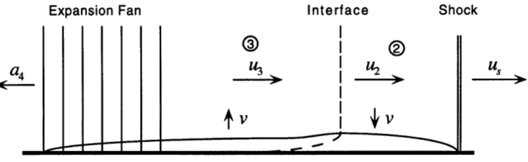
Expansion Fan Interface Shock
v
iv
Figure 2-4: Effect of boundary layer growth on shock tube flows.
sensitive to changes in reservoir temperature. For an unshrouded supersonic nozzle, the exit velocity up '$
V
and the noise power P- u/T
2 T t52.
An 8% drop in reservoirtemperature would therefore reduce the radiated noise by approximately 1 dB.
2.2
Boundary Layer Effects
The one-dimensional gas dynamic analysis of a perfect fluid presented in Section 2.1 is useful for providing a first estimate of shock tube performance. However, in real shock tubes there are viscous, thermal, and three-dimensional effects that have a significant impact on performance. The most significant of these is the unsteady growth of a boundary layer in the fluid accelerated by the shock. The generation of this boundary layer results in the attenuation of the shock, axial and transverse flow non-uniformities, acceleration of the free-stream, shock curvature, reflected shock bifurcation, and a general reduction of the test time [23].
The fluid between the expansion head and the shock wave has been accelerated from rest to a velocity u2. As a result, there will be an unsteady boundary layer growing in this region. The maximum boundary layer thickness will occur somewhere between the diaphragm and the contact surface, and will be reduced to 6 = 0 at the wave fronts as shown in Figure 2-4.
The presence of this boundary layer has a number of effects on the shock tube flow. The axial velocity, for instance, will no longer be uniform due to the restriction in flow area. More significantly, there will be a positive radial velocity, v, in region (2) producing the same effect as if the tube diameter were expanding. This generates weak pressure waves that overtake and attenuate the shock [22]. An estimate of the boundary layer thickness was made to determine the magnitude of these effects.
SHOCK U2 = U2 - Us SHOCK
u2
2,
--- U
Uw = -Us
(a) Laboratory reference frame (b) Shock stationary reference frame
Figure 2-5: Boundary layer approximated as steady flow over a semi-infinite flat plate through change of reference frame
2.2.1
Boundary Layer Model
The boundary layer is difficult to analyze due to the unsteady nature of the problem. How-ever, if a shock stationary reference frame is adopted then the problem can be approximated as a steady boundary layer growing on a moving semi-infinite flat plate, as shown in Fig-ure 2-5. This model requires that the boundary layer be thin compared to the shock tube diameter. If this is the case, than a number of simplifying assumptions can be made:
* The pressure perturbations associated with the unsteady boundary-layer growth can be ignored
* The shock attenuation can be neglected, and the inflow conditions (T2,p2,v2) can be assumed to be uniform
* The free stream velocity, v2, is independent of x; this requires 6* < Dst.
* Locally, the curved tube wall can be approximated as a flat plate. The Reynolds number can be defined as
PwU2X
Re = (2.9)
where the characteristic velocity is taken to be u2, the difference in velocity between the free stream and the wall. Similarly, the characteristic distance is taken to be x - 1i which is the distance any particle at a position x will have traveled since the passage of the shock.
- = 0.01 atm 10
-
- pi = 0.16 atm p,...P = 1.00 atm 102 10 .10 -2 10-3 1 1.5 2 2.5 3 3.5Shock Mach Number, Ms
Figure 2-6: Distance between shock and turbulent boundary layer transition point as a function of shock Mach number, M,. Circle denotes typical HSCT operating point, ps/po = 3.7, T5/To = 3.0. Ret = 4 x 10
6.
Boundary layer transition occurs in the range 5 x 10⁵ < Ret
<
4 x 10⁶ for 1<
Ms<
9 [9]. Figure 2-6 presents the location of the transition point as a function of shock Mach number. The flow will become turbulent a short distance behind the incident shock, xt 0 5 cm, at the facility design conditions, so a fully turbulent boundary layer model can be adopted. This will be a valid model for test conditions characteristic of gas turbine engine nozzles. However, if low tube pressures, pl < 0.05 atm, and relatively weak shocks, Ms < 2.0, are employed, a substantial length of the boundary layer will be laminar (see Figure 2-6) and the fully turbulent model will no longer be valid.The details of the turbulent boundary layer model are presented in Appendix B. The velocity profile was assumed to follow a power-law distribution, and the thermal boundary layer was defined using the Crocco-Busemann relation. The boundary layer thickness and wall shear forces were found using the Blausius relation for compressible turbulent flow over a semi-infinite flat plate [7].
Results of these calculations are presented in Figure 2-7 for the facility design conditions. The boundary layer model has been demonstrated to agree with experimental data to within
V.. 0.05 .
-o
-i
- 8" Shock Tube -- 12" Shock Tube 0 0 0.02 0.04 0.06 0.08 0.1 0.12 0.14 0.16 0.18 0.2 0.02 0.01 0 0.02 0.04 0.06 0.08 0.1 0.12 0.14 0.16 0.18 0.2 0.02 S0.01 0 0.02 0.04 0.06 0.08 0.1 0.12 0.14 0.16 0.18 0.2 xs / IstFigure 2-7: Boundary layer parameters in driven section for 8" and 12" shock tube facilities;
M, = 2.28, pi = 0.15 atm.
approximately 15% over this operating range [19]. As a general trend, the boundary layer effects will become more severe as the length-to-diameter ratio of the shock tube is increased and the initial driven section pressure is reduced.
2.2.2 Shock Attenuation
The attenuation of the initial shock wave can be predicted by modeling the boundary layer as a distribution of mass sources along the wall of the tube. The pressure perturbations can then be integrated along the characteristic lines to find the variation in shock strength [23]. These calculations, however, are cumbersome, and, for the relatively weak shocks required for this experiment, the attenuation will not be severe. Existing shock tubes with similar geometries and operating conditions realize 90% to 95% of the ideal shock speed [21]. For the purposes of the design, an 8% loss has been assumed. The exact number is not important because the driver pressure can be increased to account for the attenuation. It is important, however, to account for the roughly 25% higher driver pressures that will be required to compenstate for such losses when establishing the maximum pressures in the
facility.
2.2.3
Free Stream Acceleration
The presence of the boundary layer will also cause a reduction in effective flow area and,
as a consequence, variations in free-stream velocity. This change in u2 will not be uniform,
but rather a function of 6* and therefore a function of distance behind the shock. This
has the effect of tilting the expansion head toward the nozzle and decreasing the separation
between the shock and the contact surface as shown in Figure 2-9.
The variation in free-stream velocity can be estimated using the simplified boundary
layer model. The problem is approximated as a steady flow through a contracting duct
where the effective diameter is set based on the displacement thickness. This gives an
expression
P2v2 P2
Dst
(2.10)
(P2V2)o Dst - 46*
where
v2is the velocity in the shock stationary reference frame. Figure 2-8 shows the
results of this calculation transformed into the laboratory frame. It can be seen that the
free stream velocity will be increased as much at 10% at the contact surface. This will
reduce the shock-interface separation and curve the centered expansion toward the nozzle
(see Section 2.2.4).
The coupling between the free stream variations and the boundary layer growth was
neglected in this model, so the results are only approximate. A more accurate solution
can be found using a local similarity assumption and simultaneously solving for 6 and u
2[22]. However, if the boundary layer is thin compared to the tube diamter, the uniform
free-stream model is sufficient.
2.2.4
Influence of Boundary Layer on Time-Distance History
The non-ideal effects associated with the boundary layer will have a strong influence on
the time-distance history of the shock tube. Figure 2-9 illustrates qualitative differences
between real and ideal behavior based on observations from other shock tubes [23]. Some
of the differences result from the finite diaphragm bursting times and the non-uniformity of
the free stream due to boundary layer growth. However, the most significant changes are a
1.1 1.09 . 1.068 1.05. , . . 1.03 8" Shock Tube 1.02 - - 12" Shock Tube 1.01 . . 0 0.02 0.04 0.06 0.08 0.1 0.12 0.14 0.16 0.18 0.2 xs / It
Figure 2-8: Variation in free stream velocity due to boundary-layer growth behind the shock for
the 8" and 12" shock tubes; M8 = 2.28, pi = 0.15 atm.
consequence of the shock attenuation.
The shock will not follow a straight line on the wave-map. Initially it will accelerate as the diffuse compression front created by the diaphragm removal coalesces into a discrete shock. The shock will reach a maximum speed several diameters downstream, then slow down as it is attenuated by the weak rarefactions generated by the boundary layer.
As a result, in order to achieve the same reservoir conditions, a higher driver pressure will be required than predicted using the ideal model. This will generate a stronger centered expansion and cause the expansion tail to be tilted toward the nozzle. This, in turn, will cause the reflected shock to overtake the expansion tail at a lower T5
/T1
than predicted by the ideal model, significantly changing the optimum geometry. This effect can be modeled by evaluating the increase in driver pressure needed to compensate for the shock attenuation, recalculating the strength of the centered expansion using the increased diaphragm pressure ratio, and updating the time-history diagram using the trajectory of the stronger centered expansion. The relative length of the driven section, ldn/lt, should be larger than that predicted in the ideal model to make allowances for this change in gas-dynamic behavior.distance distance
(a) Ideal shock tube flow (b) Real shock tube behavior
Figure 2-9: Illustration of time-distance histories in real and ideal shock tubes used to generate equivalent reservoir conditions.
Shock
U2 Urs U5
Boundary Layer
Figure 2-10: Shock Bifurcation Structure for Re < 900, 000. Figure adapted from Mark [18]
2.2.5
Reflected Shock-Boundary Layer Interaction
After the shock reflects from the end wall, it will encounter the unsteady boundary layer and no longer behave as a simple plane wave. In laminar flows, a strong bifurcation of the shock has been observed in the region close to the shock tube walls as shown in Figure 2-10 [18]. This oblique shock structure leads to non-uniform heating across the test section and, more importantly, the mixing of driver and driven gases as the shock crosses the contact surface. This contaminates the test gas with the cold driver fluid and reduces the total test time.
In turbulent flows this effect is much less severe. The increased transport of energy from the main stream eliminates the conditions in the low-energy laminar boundary layer
107 Mp = 2.0
Mp = 1.5
S106 TranSition Reynolds Number
10s
104
1 1.5 2 2.5 3 3.5
Ms
Figure 2-11: Reynolds number at point of shock-interface interaction.
shock will be interacting with a laminar or turbulent boundary layer when it crosses the contact surface.
Turbulence transition was investigated in reference [18] using a series of Schlieren pho-tographs. It was found that the shock bifurcation structure disappeared for Reynolds num-bers over 9 x 10⁵ where
PwU2X U Urs
Re - 2X
(
+ U2 (2.11)From Figure 2-11 it can be seen that shock bifurcation will only be expected for low initial tube pressures (pl < 0.07 atm) or weak shocks (M, < 1.5). It should be noted, however, that the transition Re cited in reference [18] was based on limited data and is not nec-essarily representative of all shock strengths; experiments were conducted at Ms = 2.15. Mixer/ejector experiments in this facility will be conducted with shock Mach numbers close to this value, ranging from 2.00 < Ms < 2.25.
Mp = 3.0
2.3
Duration of Constant Conditions in Reservoir
The duration of constant conditions in the reservoir will be limited by one of two factors;
the arrival of a reflected shock or expansion at the nozzle, or the exhaustion of the test gas.
In most cases, the arrival of a reflected disturbance will be limiting. However, for large area
ratio nozzles (A*/Ast
>
0.08) or high reservoir temperatures (T
5/To
>
4.0) the volume of
test gas will be a greater constraint.
2.3.1
Wave Reflection Limited Test Times
Depending on the operating conditions and the relative lengths of the driver and driven
sections, there are three different reflections that can result in the termination of the test.
Wave diagrams for each of these conditions are shown in Figure 2-12. Each case is discussed
below.
Reflections From Contact Surface
The first disturbance that could potentially end a test results from the interaction of the
shock with the contact surface (see Section 2.1.3). This is shown schematically in Figure
2-12a. In this case, as is shown in Figure 2-13, test times will typically be in the range of
Texp = T1 e 2 to 3 milliseconds. This test time is insufficient for jet noise experiments asthe fluid jet will not have time to reach a quasi-steady state (see Section 3.3). Therefore
reflections from the contact surface must be eliminated through tailoring of the driver gas
as discussed in Section 2.1.3.
Primary Expansion Head
The second situation is shown in Figure 2-12b. The head of the primary expansion fan will
travel the length of the driver section, reflect from the end-wall, and propagate back to the
nozzle. This is a strong wave and will rapidly reduce the reservoir pressure and temperature
once it arrives. In this case, test times are in the range T3 e 14 to 20 milliseconds as shown
in Figure 2-13. The arrival of the expansion head can be delayed by increasing the relative
length of the driver section, ldr/
1st. However, the driven section must remain long enough to
insure a sufficient volume of test gas and to prevent the shock from overtaking the expansion
tail.
(a) Test time limited by reflection off in-terface
(b) Test time limited by primary expan-sion
(c) Test time limited by secondary expan- (d) Optimum shock tube geometry at
sion given Ts/T