OATAO is an open access repository that collects the work of Toulouse
researchers and makes it freely available over the web where possible
Any correspondence concerning this service should be sent
to the repository administrator:
[email protected]
This is an author’s version published in:
http://oatao.univ-toulouse.fr/18309
To cite this version:
Pérez Arroyo, Carlos and Puigt, Guillaume and
Boussuge, Jean-François and Airiau, Christophe Large
Eddy Simulation of Shock-Cell Noise From a Dual
Stream Jet. (2016) In: 22nd AIAA/CEAS Aeroacoustics
Conference, 30 May-1 June 2016 (Lyon, France)
Official URL:
https://
dx.doi.org/10.2514/6.2016-2798
Large Eddy Simulation of Shock-Cell Noise
From a Dual Stream Jet
Carlos P´
erez Arroyo
∗, Guillaume Puigt
†and Jean-Fran¸cois Boussuge
‡CERFACS, 42 avenue Coriolis, 31057 Toulouse CEDEX (France)
Christophe Airiau
§Institut de M´ecanique des Fluides de Toulouse, UMR 5502 CNRS/INPT-UPS, All´ee du Professeur Camille Soula, F31400 Toulouse (France)
This study presents the shock-cell noise results obtained with a large eddy aeroacoustic simulation from a dual stream jet. The primary stream is cold and subsonic with an exit Mach number of Mp = 0.89 and a Reynolds number of Rep = 0.57 × 10⁶. The secondary
stream is cold supersonic and under-expanded with a perfectly expanded Mach number of Ms= 1.20 and Res= 1.66 × 10⁶. The computations are performed with the structured
multi-block solver elsA. The aerodynamics and aeroacoustics of the flow are studied and analyzed in detail showing good agreement with experimental fits for the lengthscale and shear layer development. An acoustic-hydrodynamic filtering is used in order to compute the characteristic wavelengths of each component and estimate the shock-cell noise frequency. Moreover, the broadband shock-cell noise is captured in the near and far fields.
I.
Introduction
The noise perceived in the aft-cabin for a commercial airplane at cruise conditions is mainly due to the turbofan jet. Turbofan engines were initially used in the 50s and they have been evolving ever since, increasing in performance and in by-pass ratio. At non-optimal flight conditions, a pressure mismatch appears between the ambient air and the secondary stream of the turbofan engine. This imperfect expansion leads to the formation of (diamond-shaped) shock-cells that are a series of expansion and compression waves which interact with the vortical structures evolving in the mixing layer of the jet. This interaction process generates strong noise components on top of the turbulent mixing spectrum; subsequently, supersonic jets are noisier than their subsonic counterparts.1 The resulting shock-cell associated noise is radiated mainly in
the forward direction which impinges on the aircraft fuselage and it is then transmitted into the cabin. Shock-cell noise is primarily constituted of two components: the screech tonal noise and the broadband shock-associated noise (BBSAN). The first component is a tonal noise known as ’screech’. This tonal noise appears from a closed feedback loop between the generation of the vortical structures convected downstream and the perturbations propagated upstream that are generated when they interact with the shock-cell system. In single jets, screech is usually generated by the interaction with the third and the forth shock-cells.2 Tam
et al.3 demonstrated experimentally that the broadband component was originated as well due to the interaction between the vortical structures and the quasi-periodic shock-cell system. The origin of the BBSAN was located by Norum et al.4 in the downstream weaker shock-cells.
The first studies on shock-cell noise for dual stream jets was carried out by Tanna et al.5 in the 70s. It was found that the shock-cell structure and its produced noise was closely linked to the relation between the total to ambient pressure ratio of the core and the fan jets. In particular, Tanna et al.6,7 and Tam et
al.8,9 showed that having a sligthly supercritical primary jet would yield an almost complete destruction of
the shock-cell system of the secondary stream, reducing the overall shock-cell noise. Dahl et al.10,11 applied ∗Phd Student, Computational Fluid Dynamics Department, [email protected]
†Senior Researcher, Computational Fluid Dynamics Department, [email protected] ‡Project Leader, Computational Fluid Dynamics Department, [email protected] §Professor, University of Toulouse
the instability wave noise generation model of Tam et al.12,13 to supersonic dual stream jets. The structure
of the shock-cell system and the appearence and location of a shock-disk on the primary jet was studied by Rao.14 The appearance of screech on dual stream jets was studied experimentally by Bent et al.15 It was found that the ’tonal’ shock-cell noise disappeared when bifurcations where used inside the nozzle of the secondary stream. This illustrates how the effect of a pylon and the internal struts of commercial turbofans would disengage screech from being present in commercial aviation. Murakami et al.16,17 studied the lengths of the potential cones as well as the spreading angle of both the primary and the secondary jets obtaining good agreement with the theory. The constant increase in by-pass ratio and the new regulatory terms that were agreed by the community on noise reduction led to the industry to focus again on the noise generated by the turbofans. An extensive experimental campaign on subsonic and supersonic dual stream jets was initiated by Viswanathan18,19 and Viswanathan et al.20 in order to carry out a parametric study on the
effect of the primary and secondary nozzle pressure ratios, the secondary-to-primary jet velocity ratio and the secondary-to-primary nozzle area ratio. The main conclusions are summarized in the following. Firstly, the shock-associated noise strongly depends on the geometric shape of the nozzle and to whether or not the shocks appear in the primary or in the secondary jets. When the shock-cell structure appears on the secondary stream, there is a strong radiation to the aft angles. Secondly, the velocity ratio is relevant for mixing noise but insignificant for shock-cell noise obtaining the noise characteristics similar of those from a single stream jet when the ratio is less than 0.5. On the other hand, when this parameter is high enough, the contribution from the secondary jet is dominant at high frequencies and upstream angles. Lastly, the noise propagated at downstream angles remains invariant for all geometric and jet conditions. Another experimental campaign was carried out by Bhat et al.21 who concluded that even though shock-cell noise does not increase monotonically with increasing power settings,18the overall power level does.
Shock-associated noise is originated from the interaction between the vortical structures that develop in the shear layer and the cell system. When the secondary stream is imperfectly expanded, the shock-cell system is envolved by the inner and the outer shear layers. Therefore, two possible shock-associated noise sources from the interaction with both shear layers appear. Abdelhamid et al.22 found that the high
frequency components developed in the primary shear layer whereas the low frequency components originated on the secondary shear layer. This phenomena was further studied by Tam et al. who developed a model23
able to predict the shock-associated noise frequency peaks from both primary and secondary shear layer using a Fourier decomposition of the shock-cell system.24 The advances in high performance computing (HPC)
have enabled the possibility of running high Reynold large eddy simulations of dual stream jets.25,26,27,28
In this paper, the aeroacoustic analysis of a Large Eddy Simulation (LES) of a dual stream jet which has the secondary flow under-expanded is presented. The simulation was optimized in order to capture the BBSAN generated by the shock-cells. The paper is structured as follows. First, the numerical formulation of the CFD solver is mentioned in II. Then, the case of study and the procedure to obtain the results are explained in III. Third, the mesh is accurately described in IV. Forth, the results of the simulation are analyzed. The aerodynamics of the flow are analyzed in V and compared to some preliminary Particle Imaging Velocimetry (PIV) that are being carried out in the brand-new aeroacoustic jet facility29 at the von Karman Institute (VKI). The acoustic component is filtered from the hydrodynamic perturbations and analyzed with respect to the dominant wavelength for the shock-cell noise in VI. Finally, some conclusions and perspectives are explained.
II.
Numerical formulation
The full compressible Navier-Stokes equations are solved using the Finite Volume multi-block structured solver elsA (Onera’s software30). The spatial scheme is based on the implicit compact finite difference
scheme of 6th order of Lele,31 extended to Finite Volumes by Fosso et al.32 The above scheme is stabilized
by the compact filter of Visbal and Gaitonde33 of 6th order that is also used as an implicit subgrid-scale
model for the present LES. This scheme is able to capture perturbation waves when they are discretized by at least six points per wavelength. Time integration is performed by a six-step 2nd order Runge-Kutta DRP scheme of Bogey and Bailly.34 The present computation was performed with an in–house solution based on
III.
Simulation setup and procedure
The case of study is a co-axial jet where the primary flow is cold and subsonic with an exit Mach number of Mp= 0.89 (CN P R = 1.675) and the secondary stream is operated at supersonic under-expanded
conditions with a perfectly exit Mach number of Ms = 1.20 (F N P R = 2.45). Here, CN P R and F N P R
stand for Core and Fan Nozzle to Pressure Ratio respectively. The jets are established from two concentric convergent nozzles with primary and secondary diameters of Dp = 23.4mm and Ds= 55.0mm respectively.
The thicknesses of the nozzles at the exit are of 0.5mm. The Reynolds numbers based on the jet exit diameters are Rep= 0.57 × 10⁶ and Res= 1.66 × 10⁶. The conditions are summarized in table1.
D [mm] M N P R Re
Primary 23.4 0.89 1.675 0.57 × 10⁶
Secondary 55 1.20 2.45 1.66 × 10⁶
Table 1. Conditions for the primary and secondary nozzles.
The numerical computation is initialized by a Reynolds-Averaged Navier-Stokes (RANS) simulation using the Spalart-Allmaras turbulence model.35 The RANS solution is fully wall-resolved in the internal and external sections of the nozzles with a maximum wall unit (y+) of unity with 30 points on the boundary layer. The LES is then initialized from the RANS simulation keeping the inlet profiles. In order to accelerate the initialization from a steady state to a temporal resolved state, an intermediate coarse mesh of 25 × 106 cells was considered. The flow is initialized over 90 convective times (tˆ = ta∞/Dp) and then the data are
interpolated over the fine mesh explained in section IV. Before the flow could be considered as initialized, 60 supplementary convective times are done with the fine mesh to evacuate interpolation errors and let the flow adapt to the fine mesh. The final simulation is then run for 186 convective times in order to obtain the statistics. The simulation time corresponds to 80 convective times with respect to the secondary diameter (Ds). In order to increase the convergence of the results, they have been averaged in the azimuthal direction.
The boundary conditions used in the simulation are sketched in Fig. 1 (a). Non-reflective boundary conditions of Tam and Dong36 extended to three dimensions by Bogey and Bailly 37 are used at the inlets
as well as at the lateral boundaries. The exit boundary condition is based on the characteristic formulation of Poinsot and Lele.38 Additionally, sponge layers are used around the domain to attenuate exiting vorticity waves. An inflow forcing based on the vortex-ring of Bogey and Bailly 39 is applied in the interior of the subsonic nozzle to help transition to turbulence as shown in Fig. 1 (b). The vortex-ring adds divergence free disturbances to the velocity components based on a combination of azimuthal modes in the boundary layer region inside the nozzle. The inflow forcing is not applied in the interior of the secondary stream. Last, no-slip adiabatic wall conditions are used at all the wall boundaries of the nozzles. No wall turbulence models are used.
The far-field sound is obtained by means of the Ffowcs-Williams and Hawkings analogy (FWH).40 The
surface used to extrapolate the variables to the far-field is located in three concentric topological surfaces starting at r/Dp= 3, 4, 5 from the axis and growing with the mesh. The surfaces are closed on the exterior of
the secondary nozzle and open at the outlet. The cut-off mesh Strouhal is Sts≈ 6.0. In terms of frequency
(Sts= fDs/Us), this value is defined as f = a∞/(n∆), where ∆ is the cell size, a∞the speed of sound and
n the number of cells needed to resolve fluctuations with the actual numerical scheme used. The sampling frequency was set to 65 kHz which gives a sampling Strouhal higher than the mesh cut-off limit. The noise has been propagated up to a distance of 30Ds.
IV.
Mesh definition
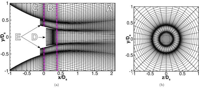
The structured multi-block mesh used for the LES is defined in this section. The mesh contains 200 × 106 cells. It consists in a butterfly type mesh in order to avoid the singularity at the axis as shown in Fig. 2
(b). Figure 2 (a) shows a gridplane at z/Ds= 0 where the capital letters [A, E] illustrate different sections
of the mesh. Section A, situated forward to the primary nozzle exit plane has roughly (1132 × 600 × 256) cells in the axial, radial and azimuthal directions respectively; there are (108 × 490 × 256) cells between the exit of the primary and secondary nozzle (section B); (172 × 326 × 256) cells over the secondary nozzle (section C) and finally, sections D and E, located inside the primary (D) and secondary nozzle (E) contain
sponge layer
non-reflective radiative conditions NSCBC farthest FW-H surface 37.5 Dp, 15.95 Ds 30 Dp, 12.7 Ds 26 Dp, 11.1 Ds 16 Dp, 7 Ds (a) vortex-ring forcing 0.75 Dp, 0.32 Ds 0.25 Dp, 1.06 Ds 3.77 Dp, 1.6 Ds 0.25 Dp, 1.06 D s (b)
Figure 1. Sketch of the numerical and physical domain in (a) a general view and (b) a detailed view.
(100 × 100 × 256) and (110 × 162 × 256) cells respectively. The lips of the nozzles are discretized with 6 cells.
x/D
sy
/D
s-1
-0.5
0
0.5
1
1.5
2
-1
-0.5
0
0.5
1
A
B
C
D
E
(a) z/Ds y /D s -1 -0.5 0 0.5 1 -1 -0.5 0 0.5 1 (b)Figure 2. Mesh grid planes representing every fourth cells in the plane (a) z/Ds = 0 and (b) the exit plane of the
primary nozzle. The capital letters [A, E] illustrate different sections of the mesh.
The walls of the internal sections of the nozzles (section D and E) as well as the external section of the primary nozzle (section B) attain a resolution at the wall of y+≈ 15 with 20 points on the boundary layers.
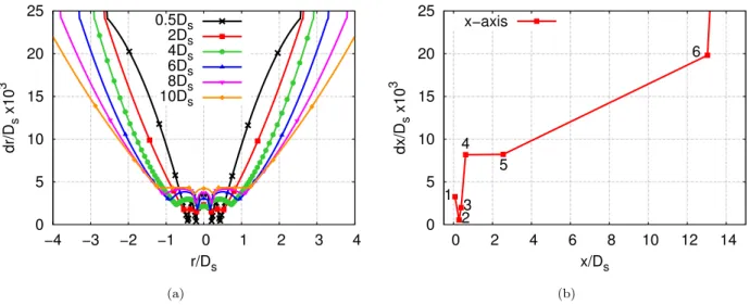
No wall turbulence models are used. The maximum expansion ratio between adjacent cells achieved in the mesh is not greater than 4%. The radial discretization at different axial positions is shown in Fig. 3(a). The maximum Helmholtz number (He = fDs/a∞) that the mesh is able to capture at the end of the physical
domain is about 5. The radial domain size grows with the axial position in order to take into account the expansion of the jet (from r/Ds = 2.5 at the exit of the primary nozzle to r/Ds = 5 at x/Ds = 13),
nonetheless, the maximum He number is kept constant at the boundary with the sponge layer. The axial discretization shown in Fig. 3 (b) is composed of 6 sections defined by the enumerated symbols. In the interior of the primary nozzle, segments 1 2 and 2 3, the mesh is refined where the vortex-ring is located (point 2). At this position, the mesh achieves an aspect ratio of 1 at the wall; this ensures an appropriate definition of the vortex-ring. At the exit of the primary nozzle (point 3), the aspect ratio of the cells at the wall attains a value of 4. In the third segment 3 4, the mesh elongates at a rate of 3%. This stretching allows for a drastic reduction of the total amount of cells in the axial direction. The segment 4 5 consists in a uniform discretization. Then, in segment 5 6, the mesh is slowly elongated up to a mesh size able to capture a Helmholtz number of 4. The last section, starting at point 6, is the one corresponding to the sponge layer where the mesh has a stretching ratio of 10%.
0 5 10 15 20 25 −4 −3 −2 −1 0 1 2 3 4 dr/D s x10 3 r/Ds 0.5Ds 2Ds 4Ds 6Ds 8Ds 10Ds (a) 0 5 10 15 20 25 0 2 4 6 8 10 12 14 1 2 3 4 5 6 dx/D s x10 3 x/Ds x−axis (b)
Figure 3. Discretization of the mesh along (a) the radial distribution for different x/Ds and (b) the axial distribution along the axis, where dr is the radial step and dx the streamwise one.
V.
Aerodynamics of the dual stream jet
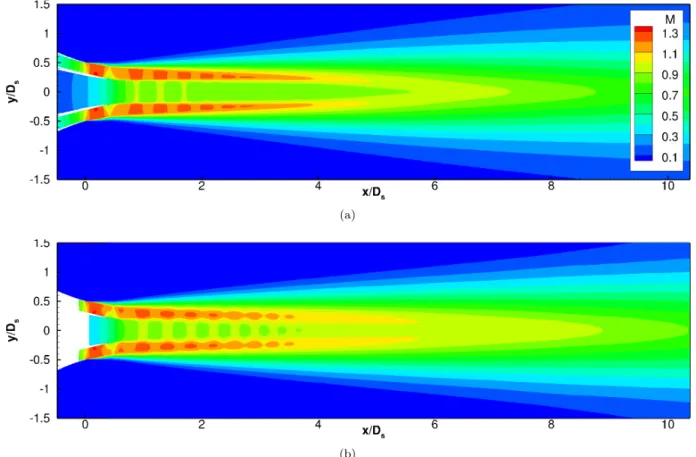
In this section the main characteristics of the flow topology as well as a comparison of the LES results with the RANS simulation are shown. The primary subsonic jet is enclosed by a supersonic under-expanded annular jet. This will create the primary potential cone surrounded by an annular potential cone where the shock-cells live as shown in Fig. 4 (a) and (b). These concentric potential cones will merge further downstream. The supersonic under-expanded secondary flow undergoes the formation of an oblique shock at the exit of the primary nozzle as it can be seen in Fig. 5(a) and (b) due to the difference in slope between the internal section of the primary nozzle and the outer section of the nozzle. This oblique shock generates a secondary shock-cell system that coexists with the one generated by the under-expanded supersonic jet at the exit of the secondary nozzle.
A supersonic under-expanded jet will expand to the ambient pressure by means of the so-called shock-cells. Its subsonic counterpart will always match the nozzle exit pressure with the ambient local pressure found outside the nozzle without the need of an expansion fan. When the local static pressure is modified with respect to the ambient pressure, the jet will actually expand to the new static pressure, modifying the actual nozzle to pressure ratio (NPR). The shape of the nozzle can modify the local pressure in its vicinity, in the same fashion as an airfoil does. Moreover, the fact that the shock-cell system position and intensity depends on the FNPR and that the flow overcomes the pressure jump of an oblique shock, it renders, a priori, impossible to maintain constant the CNPR. Therefore, in this study, the regular definition of NPR was kept, i.e. with respect to the ambient pressure and not the localized static pressure. The actual Mach number obtained at the exit of the primary nozzle achieves a value of 0.51 instead of the design value of 0.89 which is achieved after an axial distance of one primary diameter.
As it can be seen in Fig. 5, the position of the shock is slightly modified with respect to the RANS simulation due to the fact that when the expansion reaches the wall of the outer primary nozzle, it starts a small recirculation bubble. This is a side effect of the initialization of the flow with the RANS simulation without achieving the proper turbulence levels at the exit of the nozzle. The vortex-ring forcing was not used in the interior of the secondary supersonic nozzle. In order to accurately define the vortex-ring and maintain the levels of turbulence throughout the convergent nozzle, a much finer discretization and longer interior section were needed increasing the cost of the computation.
The above mentioned differences between the RANS simulation and the LES can be seen as a change of the flow variable profiles on the axis and on the central line that defines the secondary annular potential cone. Figure 6shows the Mach profiles along the (a) axis and the (b) centre-line of the secondary potential cone. It can be seen that even though a shift appears in the shock-cells, the spacing between them remains the same. As expected, the shock-cells captured by the RANS simulation are greatly reduced in amplitude due to the dissipative behavior of RANS modeling. Even though the expansion of the secondary jet into the
(a)
(b)
Figure 4. Mach contours for the (a) RANS and (b) LES mean simulations.
(a) (b)
primary jet is increased for the LES simulation as it can be seen in Fig. 6 as a Mach increment, the point of connection between both potential cones stays at the same location of x/Ds= 6.2. This position is defined
by the maximum in Mach number at the axis.
0.8 0.82 0.84 0.86 0.88 0.9 0.92 0.94 0.96 0.98 1 0 2 4 6 8 10 M y/Ds RANS LES Mean (a) 0.7 0.8 0.9 1 1.1 1.2 1.3 0 2 4 6 8 10 M y/Ds RANS LES Mean (b)
Figure 6. Mach profiles along (a) the axis of the primary nozzle and along (b) a line that follows the skewed secondary potential cone.
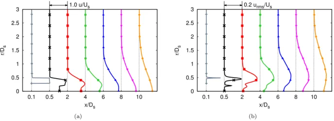
The next results will focus on the rms statistical values obtained from the LES simulation. The mean axial velocity (Fig. 7 (a)) and its rms (Fig. 7 (b)) were computed at different axial positions. The velocity jump that appears in the external secondary shear layer is halved for the internal shear layer. This has an impact on the rms, which is also halved for the primary shear layer with respect to the value at the outer shear layer. The rms peak at the secondary lipline achieves a value of 20% which is in agreement with a similar under-expanded condition of a single jet by Savarese.41 As it can be seen in Fig. 8 the −5/3 slope of the inertial range is partially recovered for the fully turbulent flow at x/Ds> 4 which assures a moderate
discretization of the mesh having a cut-off frequency above 50kHz.
0 0.5 1 1.5 2 2.5 3 0.1 0.5 2 4 6 8 10 r/D s x/Ds 1.0 u/Us (a) 0 0.5 1 1.5 2 2.5 3 0.1 0.5 2 4 6 8 10 r/D s x/Ds 0.2 urms/Us (b)
Figure 7. (a) Axial velocity profiles and (b) axial velocity rms profiles at different axial positions normalized by the exit velocity of the secondary nozzle.
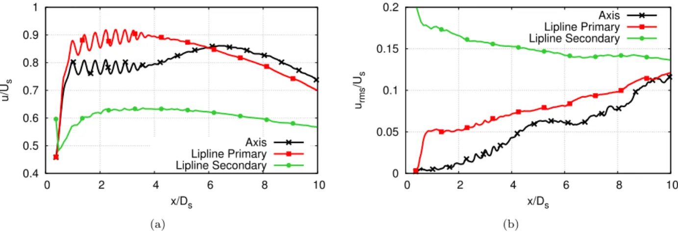
The shock-cell structure of the secondary jet affects the primary inner subsonic jet due to the change in pressure that occurs through the expansion and compression waves within the shock-cells. This change in static pressure is seen by the primary subsonic jet as a change of its ambient local pressure. Consequently, the jet tries to adapt to this new pressure. The change in pressure will affect the velocity of the primary jet with accelerations and decelerations as they occur through the shock-cells in a supersonic under-expanded jet but of course, staying in the subsonic region. This variation in velocity is clearly seen at the axis and at the primary lipline in Fig. 9 (a). The rms are shown in Fig. 9 (b). Even though the velocity at the secondary shear layer is smaller than in the primary shear layer, the rms is higher and decreases with x/Ds.
10−5 10−4 10−3 10−2 10−1 100 103 104 105 PSD u f [Hz] x/Ds= 2 x/Ds= 4 x/Dp= 6 x/Dp= 8 x/Dp=10 f−5/3 (a) 10−5 10−4 10−3 10−2 10−1 100 103 104 105 PSD v f [Hz] x/Ds= 2 x/Ds= 4 x/Dp= 6 x/Dp= 8 x/Dp=10 f−5/3 (b)
Figure 8. Power spectral density (PSD) of (a) the axial velocity u and (b) the vertical velocity v at different axial positions along the axis.
The rms at the axis and at the primary lipline increases with x/Dsuntil the three lines reach the same level
of 0.12 due to the merge of the supersonic jet with the subsonic jet as it is shown as a broadening along the radial direction of the rms in Fig. 7 (b).
0.4 0.5 0.6 0.7 0.8 0.9 1 0 2 4 6 8 10 u/U s x/Ds Axis Lipline Primary Lipline Secondary (a) 0 0.05 0.1 0.15 0.2 0 2 4 6 8 10 urms /U s x/Ds Axis Lipline Primary Lipline Secondary (b)
Figure 9. (a) Axial velocity profiles and (b) axial velocity rms profiles along the axis, the lipline of the primary nozzle, and the lipline of the secondary nozzle normalized by the exit velocity of the secondary nozzle.
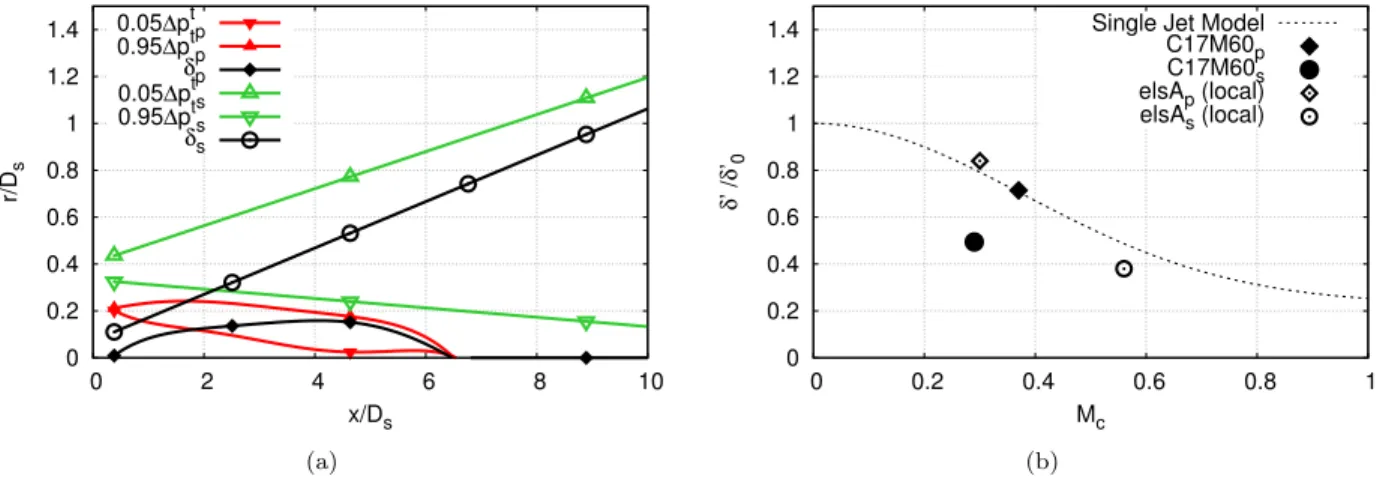
The growth rates of both primary and secondary shear layers, δp0 and δs0, are measured and compared to other coaxial jets by Murakami and Papamoschou.17 Here, the superscript 0 denotes the derivative with
respect to the streamwise direction. The growth rates are measured using as a reference the growth in Pitot thickness. The Pitot thickness represents the length of 90% of the total pressure jump ∆ptof a shear layer
formed between two flows. Figure 10 (a) shows the position of the 5% and 95% of ∆pt for the primary
shear layer with filled triangles H andN and for the secondary shear layer with hollow triangles O and 4. The growth of the shear layer is plotted with ◦ for the primary shear layer and ♦ for the secondary shear layer. The shear layer of the primary jet grows and then decreases due to the fact that the jet is engulfed by the secondary stream. The growth of the secondary shear layer is linear as it would be expected for an axisymmetric jet according to the planar shear layer model. In order to calculate the actual growth rate, one takes the derivative of the growth shown in Fig. 10(a). The growth rate of the secondary jet is constant. In order to compute the growth rate of the primary jet, the derivative of the growth was computed at the initial positions, disregarding the change in growth that the shear layer overcomes. The growth rates are compared with the experimental results for coaxial jets of Murakami and Papamoschou17in Fig. 10(b) for the case with similar area ratio between the primary and secondary jets and similar velocity ratio between the fast and the slow streams. It needs to be taken into account that in their experiments, the supersonic
jet is the primary jet. The comparison is done via the compressibility correction f (Mc) defined as: f (Mc) = δ0 δ0 0 = 0.23 + 0.77e−3.5Mc2, (1)
where Mcis the convective Mach number defined as
Uf ast−Uslow
af ast+aslow and δ
0
0is the growth rate of the incompressible
shear layer defined as C(1−r)(1+
√ s)
1+r√s . U stands for the velocity of the flow at the onset of the shear layer, a
is the speed of sound of the flow and the subindices f ast and slow define the fast and slow flows in a shear layer; r is the ratio of velocities Uslow/Uf ast and s the ratio of densities ρslow/ρf ast. The constant C was
determined by Papamoschou and Roshko42to be about 0.14. The growth rate of the primary jet δ0
p falls on
the theoretical line as the experimental results of Murakami and Papamoschou do. The secondary layer acts merely as a coflow which is well represented by the planar shear layer model. The growth is well represented when the real local values at the exit of the nozzle are used (instead of the nominal values). On the other hand, the growth rate of the shear layer of the secondary jet δ0s is deviated from the model, again, as it
happens for the experimental results, because of the lack of the interaction between both shear layers in the model. 0 0.2 0.4 0.6 0.8 1 1.2 1.4 0 2 4 6 8 10 r/D s x/Ds 0.05∆ptp 0.95∆ptp δp 0.05∆pts 0.95∆pts δs (a) 0 0.2 0.4 0.6 0.8 1 1.2 1.4 0 0.2 0.4 0.6 0.8 1 δ ’ / δ ’0 Mc
Single Jet Model C17M60p C17M60s elsAp (local) elsAs (local)
(b)
Figure 10. (a) radial positions of the inner and outer limits of the shear layer for both primary and secondary shear layers and its growth. (b) Normalized growth rate versus the convective Mach number.
The lengthscales and timescales for the axial (L11(1)) and radial velocity (L22(1)) were computed along the axis, the primary lipline and the secondary lipline and compared to those of Laurence43 and Davies et al.44
The lengthscales of the axial velocity have good agreement with the experimental fit for both the primary and secondary liplines as shown in Fig. 11 (a). The lengthscales at the axis overcome a maxima at the position of the shock-cells that oscillates with them. Then, it decreases due to the increase in axial velocity that appears with the mixing of the secondary supersonic jet. Finally it increases again and recovers the same lengthscales as the other references. A similar effect can be encountered at the primary lipline where two slopes are clearly differentiated before and after the merging with the secondary stream. As expected, the lengthscales of the radial velocity shown in Fig. 11 (b) are inferior to those computed for the axial velocity. The timescales of the axial velocity presented in Fig. 12 (a) show that they increase at two different rates, one before the merging of the potential cones and one afterwards. The maxima observed at the axis (Fig. 11(a)) is smoothed into a plateau for the timescale. On the other hand, the timescales of the radial velocity converge into the same timescales independently of the radial position as shown in Fig. 12
(b). Both lengthscales and timescales were computed as the integral of the main peak of the auto-correlation up to the first minima.
The axial velocity in the plane z/Ds = 0 is shown in Fig. 13and it is compared to some preliminary
experimental results carried out at the VKI.29 The top of the figure shows the experimental PIV results
captured with two identic IMAGER SX4M cameras set in parallel with a small overlapped region. The images were captured with a resolution of 2360 × 1766 pixels2 and a sampling frequency of 15 Hz. The
experiments were run for 40 seconds obtaining a total of 600 images. A magnification factor of 0.0498 mm/pixel and a focal ratio of 8 mm were used for the camera that was situated at a distance of about
0 0.2 0.4 0.6 0.8 1 0 2 4 6 8 10 L11 (1) / D s x/Ds Axis Lipline Primary Lipline Secondary Liepman Laufer (a) 0 0.2 0.4 0.6 0.8 1 0 2 4 6 8 10 L22 (1) / D s x/Ds Axis Lipline Primary Lipline Secondary (b)
Figure 11. Lengthscale of (a) the axial velocity u and (b) the radial velocity vr along the axis, the lipline of the
primary nozzle and the lipline of the secondary nozzle.
0 0.2 0.4 0.6 0.8 1 0 2 4 6 8 10 T11 (1) U s / D s x/Ds Axis Lipline Primary Lipline Secondary (a) 0 0.2 0.4 0.6 0.8 1 0 2 4 6 8 10 T22 (1) U s / D s x/Ds Axis Lipline Primary Lipline Secondary (b)
Figure 12. Timescale of (a) the axial velocity u and (b) the radial velocity vralong the axis, the lipline of the primary
0.5m. The interrogation windows used in the PIV were of a size of 12 × 12 pixels2 which is equivalent to 0.5976 × 0.5976 mm2. Two different experiments were done with the same conditions but with a different location of the cameras in order to obtain a bigger view of the flow donwstream. With a 50% overlap of the windows a resolution of 393 vectors is obtained. The final image, with the 4 nested frames is composed of 393 × 1085 vectors. The comparison shows that the shock-cells size computed numerically is shortened with respect to the preliminary experimental results. The first shock-cell that lives on top of the nozzle is fully attached in the experiments, however, in the numerical simulation, as it is shown in Fig. 5 (b), the flow detaches, which makes the first shock-cell being splitted in two due to the weak shock that appears due to the recirculation bubble. Nonetheless, the oblique shock that appears in the change of direction agrees well with the experiments. The positions and size of the first three shock-cells have an overall good agreement with the experiments, farther downstream, the shock-cells differ with the experiments showing a lagging in space. The size of the potential cone and the expansion of the jet matches with the experimental results even though the size of the shock-cells and thus, the number, is not the same.
Figure 13. Contour plots of the axial velocity in m/s. PIV results from29on the top of the figure and the numerical LES on the bottom.
VI.
Acoustics of the dual stream jet
As explained in the introduction, shock-cell noise appears from the interaction between the vortices developed in the mixing layer and convected downstream, and the shock-cell system that appears from the mismatch in pressure at the exit of the nozzle. The frequency of the main peak of the broadband shock-cell noise (BBSAN) can be easily calculated with the convection velocity of the vortices and the spacing of the shock-cells as fp= Uc Lsh 1 1 − Mccos(θ) , (2)
where Uc is the convection velocity, Lsh is the averaged shock-cell spacing, θ is the angle with respect to
the jet axis and Mc is the convective Mach number defined as Uc/a∞ where a∞ is the ambient speed of
sound. The fundamental frequency Uc
Lsh
that appears from the interaction of the vortices and the shock-cell system is shifted due to the Doppler effect by the factor 1−M1
ccos(θ). The Doppler effect can be seen as the
noise produced by an array of phased monopoles situated on the shock-cells that radiate noise only when the vortices interact with them. Thus obtaining a lower frequency at the upstream angles and a higher frequency at the downstream angles.
The shock-cell spacing for each shock-cell can be computed using the same formula as Harper-Bourne and Fisher,45
Ln= L1− (n − 1)∆L, (3)
where Lnis the shock-cell spacing of the n − th shock-cell and ∆L is the shock-cell spacing increase between
two consecutive shock-cells. A value of ∆L/L1≈ 0.056 is obtained which is in agreement with the results of
Harper-Bourne and Fisher45of ∆L/L
1≈ 0.060. In a single jet, the shock-cell spacing is non-dimensionalized
by the diameter of the nozzle, in this work, as the under-expanded jet is issued from the secondary nozzle, the shock-cell spacing is non-dimensionalized by the difference of the secondary and the primary diameter Dsp= Ds−Dp. This diameter is used as the shock-cells will be reflected between the secondary and the inner
shear layers. If different jet conditions are to be taken into account, the shock constant β =qM2 j − M
2 d is
also used in the non-dimensionalization, where Mj is the perfectly expanded Mach number and Md is the
actual Mach number. Here, Mj = Ms= 1.20 and Md = 1.0. Harper-Bourne and Fisher45 found a value of
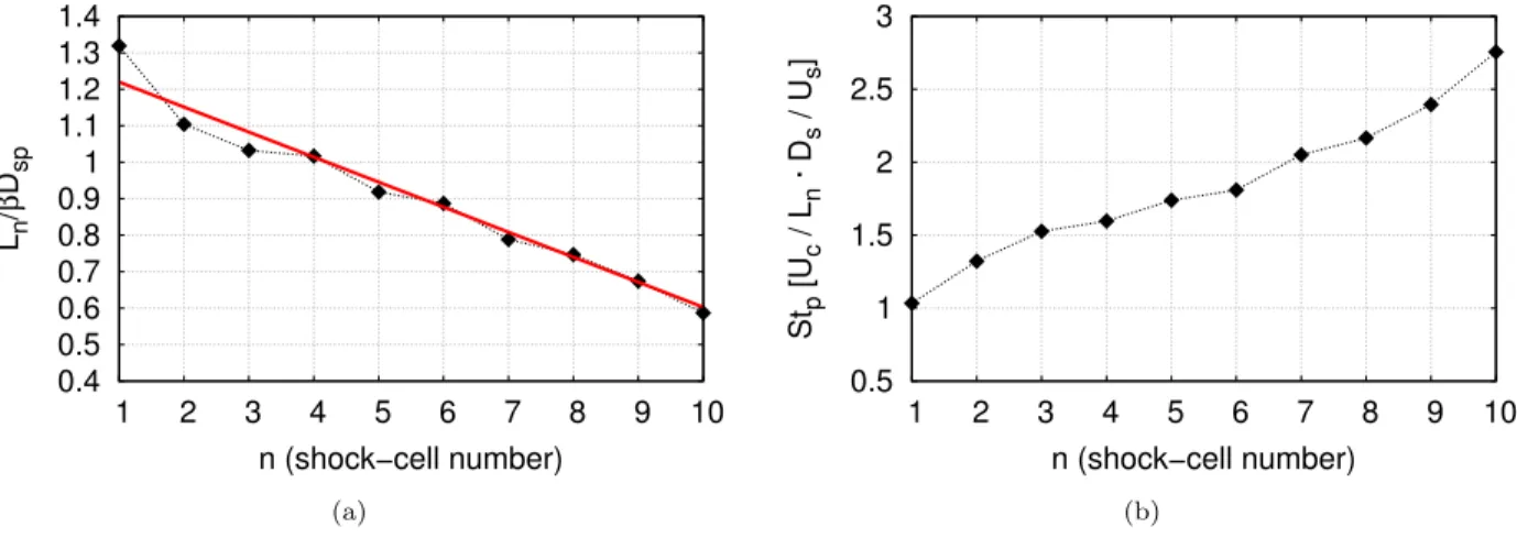
L1/(βD) ≈ 1.31; in this work, a value of 1.22 is found with the linear regression whereas the actual value is
1.32. The non-dimensional shock-cell spacing obtained in the current configuration is shown in Fig. 14(a). As it can be seen, the bias with respect to the linear regression is higher for the first shock-cells. This result is to be expected as first, the flow is not issued parallel to the axis but with an angle due to the geometry of the secondary nozzle, second, the first shock-cells interact with the oblique shock that appears at the position of the exit of the primary nozzle shown in Fig. 5 and finally, the inner subsonic jet might slightly change the topology of the shock-cells.
A good estimation of the shock-cell spacing is required in order to measure the frequency based on the convective velocity and the shock-cell spacing fsh = Uc/Lsh. However, not the shock-cell spacing nor the
convective velocity are constants. The resulting frequency will vary according to the actual parameters. Here, the convective velocity Uc has been chosen as that of the secondary lip-line shown in Fig. 9 (a). The
same convective velocity is recovered when measuring the velocity spatio-temporal correlations between two points in the secondary lip-line. The frequencies fshare shown in Fig. 14(b) and they have been computed
at the centre of each shock-cell, using an averaged convective velocity computed between the ends of each shock-cell. If an averaged shock-cell spacing Lsh of 0.34Ds and convective velocity Uc of 0.62Us are used,
a value of fsh ≈ 1.82 is recovered. As it was experimentally confirmed by Norum and Seiner,4 BBSAN is
generated in the last shock-cells. At those positions a frequency fshbetween 1.75 and 2.25 is obtained. The
mean fshfalls well into this range showing not to be a bad approximation.
0.4 0.5 0.6 0.7 0.8 0.9 1 1.1 1.2 1.3 1.4 1 2 3 4 5 6 7 8 9 10 Ln / βD sp n (shock−cell number) (a) 0.5 1 1.5 2 2.5 3 1 2 3 4 5 6 7 8 9 10 Stp [U c / L n · D s / U s ] n (shock−cell number) (b)
Figure 14. (a) Shock-cell spacing Ln/βDsp for each shock-cell where Ln is the shock-cell spacing of the n − th
shock-cell, β is the shock parameter and Dsp = Ds − Dp. (b) Strouhal of the frequency fsh= Uc/Ln.
The near-field flow is composed of hydrodynamic and acoustic perturbations. In order to focus the study in either one or the other, the acoustic-hydrodynamic filtering of Tinney and Jordan46 was performed. The
filtering can be performed outside the jet where a null mean velocity is recovered. The filtering was applied on an azimuthal array of 16 probes located at 0.85Dsfrom the axis at the secondary nozzle exit plane which
array p(x0, t) is transformed into the wavelength - frequency domain by p(k, ω) =
Z Z
p(x0, t)W (x0)e−j(kx0+ωt)dx0dt, (4)
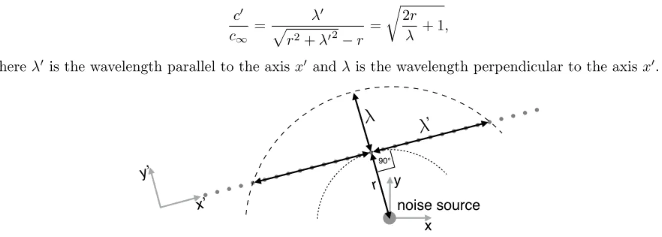
where the reference coordinate x0 is set parallel to the array. W (x0) is a weight function used to smooth the signal at the ends of the array in the axial direction. An acoustic fluctuation generated by a noise source inside the jet will be propagated outside the jet at the ambient sound speed c∞. However, the acoustic
perturbation will be propagated at a supersonic speed c02 = c∞(2rf + c∞) in the x0 coordinate system,
where r is the perpendicular distance from the axis situated on the array to the noise source and f is its frequency. Alternatively, the propagation speed seen by the axis x0 can be geometrically linked to the
perpendicular and parallel wavelengths of the noise source that emits at a frequency f = c∞/λ. The different
wavelengths and distances are sketched in Fig. 15. The propagation speed is then
c0 c∞ = λ 0 p r2+ λ02− r = r 2r λ + 1, (5)
where λ0 is the wavelength parallel to the axis x0 and λ is the wavelength perpendicular to the axis x0.
90° noise source x’ y’ x y
λ
λ
’ rFigure 15. Sketch showing the different wavelengths with respect to different axes from a noise source situated at a distance r from the array.
The hydrodynamic-acoustic filtering has been carried out on the probes located in the near-field at {0.85Ds, 1.3Ds, 1.7Ds} from the axis at the secondary nozzle exit plane with an expansion angle of 8◦.
Figure 16shows the transformed signal into k − ω with Eq. 4. The transformed signal has been averaged azimuthally in order to increase the accuracy of the figures. When the signal is transformed in to k − ω, the region that lays within the acoustic lines represents the acoustic content of the signal. Here, they are illustrated with a solid line and a dashed line for the positive and negative ambient sound speed ±c∞
respectively. The region that lays outside represents the hydrodynamic perturbations. The dotted line illustrates the above mentioned convective velocity 0.62Us. Some conclusions can be drawn from Fig. 16.
Firstly, Fig. 16 (a) shows that the hydrodynamic lobe follows the convective velocity of the secondary jet, which shows an independence of the nearfield with the primary flow. This could be expected, as the energy content of the secondary supersonic flow is much higher than that of the primary subsonic jet. The lobe corresponding to the primary jet convective velocity may lay underneath the one of the secondary jet. This is an expected different behavior with respect to a subsonic dual-stream jet46 where both lobes are clearly
present. Secondly, as expected, the hydrodynamic lobe is reduced when the probe is farther away from the axis as it is shown in Fig. 16 (a,b,c). The shape of the k − ω distribution gives information about the dispersion of the pressure fluctuations. In a non-dispersive media the energy of the convective eddies would lay aligned perfectly with the convective velocity instead of having a lobe. The amount of dispersion with respect to the convective line, gives an idea of how the perturbations can be seen as frozen. Due to this dispersion, some hydrodynamics components would lie on the acoustic side of the k − ω distribution and vice-versa. The energy of the acoustic component is spread over a wide range of k because of the location of the sources inside the jet. The acoustic content is clearly higher with respect to the subsonic jet of Tinney and Jordan46 due to the fact that here, the acoustic captured is mostly due to the shock-cell noise that is
being propagated upstream with a higher intensity whereas in a subsonic jet, it is generated by the mixing noise of fine-scale turbulence.
The subsonic and supersonic components, i.e. the hydrodynamic and acoustic components can be recov-ered from the transformed signal obtained by Eq. 4using only the ranges p(ω/k < c∞) and p(ω/k > c∞)
(a) (b)
Figure 16. k − ω representation of the nearfield flow at the probes located at (a) 0.85Ds and (b) 1.7Ds from the axis.
The solid and dashed lines represent the speed of sound. The dotted line represents the convective velocity.
respectively as: ph(x0, t) = Z p(ω/k < c∞)e−j(kx 0+ωt) dkdω, (6) pa(x0, t) = Z p(ω/k > c∞)e−j(kx 0+ωt) dkdω, (7)
where the subscript h•ihrepresents the hydrodynamic perturbations characterized by subsonic phase veloc-ities and the subscript h•ia the acoustic perturbations characterized by supersonic phase velocities. Figure
17(a), (b) and (c), show the original signal, the hydrodynamic signal and the acoustic signal respectively. The hydrodynamic signal, that is clearly appreciated in the Fig. 17(b), shows that it is well aligned with the convective speed Uc = 0.62Us represented by the solid black line as it appeared on the hydrodynamic
lobe on Fig. 16(b). As expected, some acoustic components travelling upstream are still present due to the dispersion of the signal at different frequencies. The acoustic component travels upstream and downstream at different phase velocities greater than the sound speed c∞.
(a) (b) (c)
Figure 17. Pressure on a single probe of an azimuthal array of 16 probes located at 0.85Ds from the axis which
extends up to 10Ds in the axial direction with an expansion angle of 8◦. (a) Full signal, (b) hydrodynamic component
and (c) supersonic component.
Once the flow has been filtered in hydrodynamic and acoustic components, the spatial pressure cross-correlation is studied for the original signal, and both filtered components. The spatial pressure cross-correlation gives not only information about the spatial size of the large turbulence structures, i.e. the wavelength of the wave like pattern produced by the convected vortices but it also gives information about the characteristic acoustic wavelength being seen at each position of the array. This is done by computing
the spatial cross-correlation on the hydrodynamic and the acoustic components separately. The spatial cross-correlation Rpp is computed as
Rpp=
p0(x, t)p0(x + ξ, t)
prms(x, t)prms(x + ξ, t), (8)
where p0 is the pressure perturbation, prms the pressure root mean square, x is the actual position, and
ξ the spatial separation. Figure 18 shows the cross-correlation carried out at 3 different reference points along the axial direction averaged with all the azimuthal probes. The first point presented in Fig. 18(a) is located at x/Ds= 0.85 and it shows that the acoustic correlation gives the same result as the original signal.
At this axial position, the signal is mostly acoustics originated at the shock-cells due to the fact that the hydrodynamic disturbances have not still fully developed. Farther downstream of the jet, at x/Ds= 2.6 Fig.
18(b) the acoustic correlation starts to deviate from the original signal. In particular, the negative side lobes around the maxima are closer together. At this location, the hydrodynamic disturbances are fully developed which can be seen from the bigger negative lobes typical from a train of vortices. The last position shown in Fig. 18 (c) is located at x/Ds = 4.2. At this position, the three correlations are fully different which
shows the importance of a hydrodynamic-acoustic separation of the flow when the measures are done close to the jet. Nonetheless, the three cross-correlations share a common crossing point which shows that the cross-correlation of the original signal keeps the main features of both the acoustics and the hydrodynamics of the flow. −0.4 −0.2 0 0.2 0.4 0.6 0.8 1 0 0.5 1 1.5 2 Rpp x/Ds Full Hydrodynamic Acoustic (a) −0.4 −0.2 0 0.2 0.4 0.6 0.8 1 1 1.5 2 2.5 3 3.5 4 4.5 5 Rpp x/Ds Full Hydrodynamic Acoustic (b) −0.4 −0.2 0 0.2 0.4 0.6 0.8 1 2 3 4 5 6 7 Rpp x/Ds Full Hydrodynamic Acoustic (c)
Figure 18. Azimuthally averaged pressure cross-correlation of an azimuthal array of 16 probes located at 0.85Ds from
the axis which extends up to 10Ds in the axial direction with an expansion angle of 8◦. Cross-correlations centered
at (a) x/Ds= 1, (b) x/Ds= 2 and (c) x/Ds= 3.
The characteristic wavelength λ shown in Fig. 19(a) can be computed by measuring the distance between the negative peaks around the maxima of the correlations. As expected the characteristic wavelength of the acoustic component clearly differs from the one of the hydrodynamic component. On the other hand, even though the cross-correlation shown in Fig. 18 are mostly different for the original signal and the two components, the characteristic wavelength of the original signal appears to be similar to the one of the hydrodynamic component. The characteristic frequency can be computed from the characteristic wavelength by setting a characteristic phase velocity as f = Uref/λ. The phase velocity chosen for the hydrodynamic
component is the convection velocity Uc = 0.62Us. When dealing with the acoustic component, special
attention should be given to the reference phase velocity. As it is shown by the sketch of Fig. 15, the characteristic wavelength λ0 along the axis x0is the one that is being computed when measuring the distance between the negative peaks. Moreover, as it is shown by Eq. 5 the phase velocity c0 on the same axis varies with the wavelength. The frequency is therefore computed as
f = c 0 λ0 = λ0c∞ λ0pr2+ λ02− r = c∞ p r2+ λ02− r, (9)
where λ0 on the numerator has been simplified with the λ0 used to compute the frequency f. Here, r being the perpendicular distance from noise source to the array, it grows with x as the array has an expansion angle of 8 degrees. The resulting frequencies shown in Fig. 19(b) give information about the peak frequencies of the convected vortices and the broadband shock-cell noise. The frequency of the hydrodynamic component starts at St = 0.65 but it decays up to a value of St = 0.17. On the other hand, the acoustic component
shows good agreement with the frequency estimated by the mean shock-cell frequency fsh ≈ 1.82. The
reader needs to keep in mind that Eq. 9is an approximation due to the fact that it only takes into account the Doppler effect of the shock-cell noise in the measured λ0 but not in the fact that the noise comes from
several noise sources distributed along the shock-cells.
0 0.5 1 1.5 2 2.5 3 3.5 4 0 1 2 3 4 5 6 7 λ/D s x/Ds Full Hydrodynamic Acoustic (a) 0 0.5 1 1.5 2 2.5 3 0 1 2 3 4 5 6 7 Sts [f · D s / U s ] x/Ds Hydrodynamic Acoustic (b)
Figure 19. (a) Characteristic wavelength computed with the spatial cross-correlation of an azimuthal array of 16 probes located at 0.85Ds and (b) the associated frequency with a reference phase velocity.
The estimated frequency computed with Eq. 5can be compared to the actual sound pressure level (SPL) computed for each component. Here, the standard reference pressure of 2 · 10−5P a has been used. Figure20
shows the SPL in dB/Hz computed for the original signal (a), the hydrodynamic component in (b) and the acoustic component in (c). The frequencies shown in19(b) are superimposed. Good agreement is found for both the acoustic and the hydrodynamic frequencies which confirms the validity of this approach.
(a) (b) (c)
Figure 20. Sound pressure level of an array of probes located at 0.85Ds from the axis which extends up to 10Ds in
the axial direction with an expansion angle of 8◦. (a) Full signal, (b) hydrodynamic component and (c) supersonic
component.
The SPL have been computed as well for the acoustic component in the near-field at the arrays located at {0.85Ds, 1.3Ds, 1.7Ds} The shock-cell noise is shown in Fig. 21 centered around Sts = 2, x/Ds = 2
highlighted with the dashed circle. This ’banana shaped’ signature was already encountered by Savarese41 for a supersonic under-expanded jet. At the closest position to the axis, there are some higher frequency
components that overlap with the shock-cell noise. This high frequency noise is related to the vortex pairing that occurs at the exit of the nozzle. The amplitude has the same order of magnitude as the shock-cell noise due to the fact that the flow overcomes transition in less than half a diameter. A fully turbulent flow at the exit of the nozzle, would have reduced this noise component, however, the computational cost was too expensive.
(a) (b) (c)
Figure 21. Acoustic component of the nearfield in dB/Hz along different axial positions for a line array with an angle of 7.3◦ at (a) r/D
s = 0.85, (b) r/Ds = 1.3 and (c) r/Ds = 1.7.
The pressure perturbations in the near-field were propagated to the far-field by means of the FWH analogy as explained in III. The noise was propagated to 30Dsfrom the primary nozzle exit at an exit angle
between 20 and 160 degrees. Figure 22shows the spectra for different angles. As it was explained by Tam et al.,23 two broadband contributions should be present in the spectra. One broadband component that
emanates from the interaction between the shock-cell system and the vortical structures of the secondary exterior shear layer. This component acts mostly as the BBSAN found in single jets,1 that is, its main
directivity is upstream and the peak widens for smaller angles. The second component appears from the interaction between the shock-cell system and the vortical structures from the internal primary shear layer. Opposite to the first component, the main directivity is downstream and it has a lower amplitude than the first component. Figure 22(b) shows that the peak of the main broadband contribution corresponding to the interactions between the secondary shear layer and the shock-cell system is the one captured and its directivity is well upstream. On the other hand, the secondary contribution of the interactions of the shock-cell system with the primary shear layer is not recovered.
VII.
Conclusions
and perspectives
A large eddy simulation of a supersonic under-expanded axisymmetrical dual stream jet was carried out showing the ability to qualitatively capture the broadband shock-cell associated noise generated by the interaction of the large structures and the shock-cell system that appears in the secondary under-expanded stream. The jet topology was studied and compared with the RANS simulation obtaining good agreement between them. At the exit of the primary nozzle, a localized pressure difference with respect to the ambient pressure occurs due to the appearance of the shock-cell system and of an oblique shock on the secondary stream. The oblique shock appears due to the abrupt change in direction of the flow at the exit of the primary nozzle and around it. The impact of the pressure difference is highlighted as a difference in nozzle to pressure ratio with respect to the nominal values. Furthermore, the shock-cell system of the secondary stream modifies the pressure and velocity components of the primary stream. The lengthscales computed
along the liplines follow the experimental fits of Laurence and Davies et al.. The growth rate of the secondary shear layer is in agreement with previous studies and the theoretical approach. Good agreement is found in the development of the jet with some preliminary PIV studies carried out at VKI. The nearfield flow has been filtered into acoustic and hydrodynamic components obtaining good agreement with the convective velocity of the secondary stream for the hydrodynamic part. The wavelength has been computed for the acoustic and hydrodynamic component using spatial cross-correlations. Good agreement is found when the wavelength are used to estimate the main frequency of the peaks of the broadband shock-cell noise with the phase velocity obtained from the acoustic-hydrodynamic filtering. The shock-cell noise is captured and propagated to the far-field by means of the Ffowcs-Williams and Hawkings analogy. The main contribution coming from the secondary stream emerges, however, the possible contribution coming from the primary stream as explained by Tam, is invisible with the actual post-processing techniques. The intensity of this shock-cell noise could be below the amplitude of the main bump and thus it remains hidden. The results obtained so far are encouraging for future works. Nonetheless, they are still to be thorougly compared with experimental data in terms of flow development and acoustics.
Both quantity and quality of jet noise research using Large Eddy Simulations have increased during the last fifteen years, together with a huge improvement of the results. The development of new optimized and adapted numerical schemes, an increase in computational power and new post-processing techniques have allowed for a better understanding in jet noise. In relation to this work, the modeling of the nozzle should be further improved, going deeper inside the nozzle in order to obtain a better turbulent boundary layer at its exit. In order to accomplish this goal, new wall–turbulence models adapted to high–order compact schemes47
should be applied in order to avoid a costly wall–resolved mesh but yet, achieving a good representation of the boundary layer. Moreover, a less dissipative filter of order eight should be used in the future to better capture the pressure perturbations. In addition, the aeroacoustics simulations of supersonic non–perfectly expanded jets need an efficient shock capturing technique. The present computation was performed with an in–house solution based on a limiter near the shock. Further improvements were proposed recently and their effects will be analysed in the near future. The geometry taken into account in this work is a simple sketch of a complex industrial case. In the future, a more complex geometry will be considered, including for example, the loss of symmetry due to the inclusion of the pylon inside the nozzle and the addition of a wing to take into account noise reflexions to the ground. These kind of step-by-step additions are compulsory in order to end up with a well modeling of the Ultra High Bypass Ratio (UHBR) turbofans of the next generation of airplanes.
Acknowledgments
This research project is supported by a Marie Curie Initial Training Networks (ITN) AeroTraNet 2 of the European Community’s Seventh Framework Programme (FP7) under contract number PITN-GA-2012-317142 that aims to generate a ready-to-use model for shock-cell noise characterization. This work was performed using HPC resources from GENCI - [CCRT/CINES/IDRIS] (Grant 2016-[x20162a6074]). The authors are thankful to Onera for licensing CERFACS to use the code elsA.
References
1Tam, C. K. W., “Supersonic jet noise,” Annu. Rev. of Fluid Mech., Vol. 27, No. 1, 1995, pp. 17–43.
2Krothapalli, A., Hsia, Y., Baganoff, D., and Karamcheti, K., “The role of screech tones in mixing of an underexpanded
rectangular jet,” J. Sound Vib., Vol. 106, No. 1, 1986, pp. 119–143.
3Tam, C. K. W. and Tanna, H. K., “Shock associated noise of supersonic jets from convergent-divergent nozzles,” J. Sound
Vib., Vol. 81, No. 3, 1982, pp. 337–358.
4Norum, T. D. and Seiner, J. M., “Broadband shock noise from supersonic jets,” AIAA J., Vol. 20, No. 1, 1982, pp. 68–73. 5Tanna, H. K., Tester, B. J., and Lau, J. C., “The noise and flow characteristics of inverted-profile coannular jets,” Tech.
rep., National Aeronautics and Space Administration, Langley Research Center, 1979.
6Tanna, H. K. and Brown, W. H., “Shock Associated Noise Reduction From Inverted-Velocity-Profile Coannular Jets,”
NASA Tech. Mem., 1981.
7Tanna, H. K., Brown, W. H., and Tam, C. K. W., “Shock associated noise of inverted-profile coannular jets, Part I:
Experiments,” J. Sound Vib., Vol. 98, No. 1, 1985, pp. 95–113.
8Tam, C. K. W., “Shock associated noise of inverted-profile coannular jets, Part III: Shock structure and noise
9Tam, C. K. W. and Tanna, H. K., “Shock associated noise of inverted-profile coannular jets, part II: Condition for
minimum noise,” J. Sound Vib., Vol. 98, No. 1, 1985, pp. 115–125.
10Dahl, M. D. and Morris, P. J., “Noise from supersonic coaxial jets, part 1: Mean flow predictions,” J. Sound Vib.,
Vol. 200, No. 5, 1997, pp. 643–663.
11Dahl, M. D. and Morris, P. J., “Noise from supersonic coaxial jets, part 2: normal velocity profile,” J. Sound Vib.,
Vol. 200, No. 5, 1997, pp. 665–699.
12Tam, C. K. W. and Burton, D. E., “Sound generated by instability waves of supersonic flows. Part 1. Two-dimensional
mixing layers,” J. Fluid Mech., Vol. 138, 1 1984, pp. 249–271.
13Tam, C. K. W. and Burton, D. E., “Sound generated by instability waves of supersonic flows. Part 2. Axisymmetric jets,”
J. Fluid Mech., Vol. 138, 1 1984, pp. 273–295.
14Rao, T. V. R., Kumar, R. R., and Kurian, J., “Near field shock structure of dual co-axial jets,” Shock Waves, Vol. 6,
No. 6, 1996, pp. 361–366.
15Bent, P. H., Blackner, A. M., Newsum, S. A., and Nesbitt, E. H., “Shock associated noise of dual flow nozzles,” AIAA
J., Vol. 2323, 1998.
16Murakami, E. and Papamoschou, D., “Mean flow development in dual-stream compressible jets,” AIAA J., Vol. 40, No. 6,
2002, pp. 1131–1138.
17Murakami, E. and Papamoschou, D., “Mixing layer characteristics of coaxial supersonic jets,” AIAA J., Vol. 2060, 2000,
pp. 1–16.
18Viswanathan, K., “Parametric study of noise from dual-stream nozzles,” J. Fluid Mech., Vol. 521, 2004, pp. 35–68. 19Viswanathan, K., “True Farfield for Dual-Stream Jet Noise Measurements,” AIAA J., Vol. 49, No. 2, 2011, pp. 443–447. 20Viswanathan, K., Czech, M. J., and Lee, I. C., “Towards Prediction of Dual-Stream Jet Noise: Database Generation,”
AIAA J., Vol. 49, No. 12, 2011, pp. 2695–2712.
21Bhat, T. R. S., Ganz, U. W., and Guthrie, A., “Acoustic and flow field characteristics of shock-cell noise from dual flow
nozzles,” 11th AIAA/CEAS Aeroacoustics Conference, 23–25 May, Monterey, California AIAA Paper 2005–2929 , 2005.
22Abdelhamid, Y. A. and Ganz, U. W., “Prediction of Shock-Cell Structure and Noise in Dual Flow Nozzles,” 13th
AIAA/CEAS Aeroacoustics Conference (28th AIAA Aeroacoustics Conference), 21–23 May, Rome, Italy, AIAA Paper 2007– 3721 , 2007.
23Tam, C. K. W., Pastouchenko, N. N., and Viswanathan, K., “Broadband shock-cell noise from dual stream jets,” J.
Sound Vib., Vol. 324, No. 3, 2009, pp. 861–891.
24Tam, C. K. W., Pastouchenko, N. N., and Viswanathan, K., “Computation of shock cell structure of dual-stream jets for
noise prediction,” AIAA J., Vol. 46, No. 11, 2008, pp. 2857–2867.
25Shur, M. L., Spalart, P. R., Strelets, M. K., and Garbaruk, A. V., “Further steps in LES-based noise prediction for
complex jets,” 44th AIAA Aerospace Sciences Meeting and Exhibit, 9–12 January, Reno, Nevada, AIAA Paper 2006–485 , 2006.
26Shur, M. L., Spalart, P. R., and Strelets, M. K., “Noise prediction for underexpanded jets in static and flight conditions,”
AIAA J., Vol. 49, No. 9, 2011, pp. 2000–2017.
27Viswanathan, K., Spalart, P. R., Czech, M. J., Garbaruk, A., and Shur, M., “Tailored nozzles for jet plume control and
noise reduction,” AIAA J., Vol. 50, No. 10, 2012, pp. 2115–2134.
28Sanjos´e, M., Fosso Pouangu´e, A., Moreau, S., Wang, G., and Padois, T., “Unstructured LES of the baseline EXEJET
dual-stream jet,” 20th AIAA/CEAS Aeroacoustics Conference, 16–20 June, Atlanta, Georgia, AIAA Paper 2014–1155 , 2014.
29Guariglia, D., Carpio, A. R., and Schram, C., “Design of a Facility for Shock-Cells Noise Experimental Investigation on
a Subsonic/Supersonic Coaxial Jet,” 22nd AIAA/CEAS Aeroacoustics Conference, May 30 – June 1, Lyon, France, AIAA Paper , 2016.
30Cambier, L., Heib, S., and Plot, S., “The Onera elsA CFD software: input from research and feedback from industry,”
Mech. & Ind., Vol. 14, No. 03, 2013, pp. 159–174.
31Lele, S. K., “Compact finite difference schemes with spectral-like resolution,” J. Comput. Phys., Vol. 103, 1992, pp. 16–42. 32Fosso-Pouangu´e, A., Deniau, H., Sicot, F., and Sagaut, P., “Curvilinear Finite Volume Schemes using High Order Compact
Interpolation,” J. Comput. Phys., Vol. 229, No. 13, 2010, pp. 5090–5122, jx.
33Visbal, M. R. and Gaitonde, D. V., “On the Use of Higher-Order Finite-Difference Schemes on Curvilinear and Deforming
Meshes,” J. Comput. Phys., Vol. 181, 2002, pp. 155–185.
34Bogey, C. and Bailly, C., “A family of low dispersive and low dissipative explicit schemes for flow and noise computations,”
J. Comput. Phys., Vol. 194, No. 1, 2004, pp. 194–214.
35Spalart, P. R. and Allmaras, S., “A one-equation turbulence model for aerodynamic flows,” 30th Aerospace Sciences
Meeting and Exhibit, 6–9 January, Reno, Nevada (1992), AIAA Paper 1992–0439 , 1992.
36Tam, C. K. W. and Dong, Z., “Radiation and outflow boundary conditions for direct computation of acoustic and flow
disturbances in a nonuniform mean flow,” J. Comput. Phys., Vol. 4, No. 02, 1996, pp. 175–201.
37Bogey, C. and Bailly, C., “Three-dimensional non-reflective boundary conditions for acoustic simulations: far field
for-mulation and validation test cases,” Acta Acust., Vol. 88, No. 4, 2002, pp. 463–471.
38Poinsot, T. J. and Lele, S. K., “Boundary Conditions for Direct Simulations of Compressible Viscous Flows,” J. Comput.
Phys., Vol. 101, 1992, pp. 104–129.
39Bogey, C. and Bailly, C., “Effects of Inflow Conditions and Forcing on Subsonic Jet Flows and Noise.” AIAA J., Vol. 43,
No. 5, 2005, pp. 1000–1007.
40Farassat, F. and Succi, G. P., “The prediction of helicopter rotor discrete frequency noise,” American Helicopter Society,
41Savarese, A., Jordan, P., Girard, S., Royer, A., Fourment, C., Collin, E., Gervais, Y., and Porta, M., “Experimental study
of shock-cell noise in underexpanded supersonic jets,” 19th AIAA/CEAS Aeroacoustics Conference, Aeroacoustics Conferences, 27–29 May, Berlin, Germany, AIAA Paper 2013-2080 , 2013.
42Papamoschou, D. and Roshko, A., “The compressible turbulent shear layer: an experimental study,” Journal of Fluid
Mechanics, Vol. 197, 1988, pp. 453–477.
43Laurence, J. C., “Intensity, scale, and spectra of turbulence in mixing region of free subsonic jet,” Tech. rep., 1956. 44Davies, P. O. A. L., Fisher, M. J., and Barratt, M. J., “The characteristics of the turbulence in the mixing region of a
round jet,” J. Fluid Mech., Vol. 15, No. 03, 1963, pp. 337–367.
45Harper-Bourne, M. and Fisher, M. J., “The noise from shock waves in supersonic jets,” Adv. Group Aero. Res. Dev.,
1973, AGARD Conference on Noise Mechanisms.
46Tinney, C. E. and Jordan, P., “The near pressure field of co-axial subsonic jets,” J. Fluid Mech., Vol. 611, 2008, pp. 175–
204.
47Le Bras, S., Deniau, H., Bogey, C., and Daviller, G., “Development of compressible large–eddy simulations combining
high–order schemes and wall modeling,” 21st AIAA/CEAS Aeroacoustics Conference, 22–26 June, Dallas, Texas, AIAA Paper2015–3135 , 2015.
1 2 3 4 5 6 7 8 9 10
SPL [dB/Hz]
St [f · D
s
/ U
s
]
10 dB
θ
= 30°
θ
= 90°
θ
= 150°
Figure 22. (a) Nearfield PSD at 3Dp. (b) Farfield noise at 30Ds propagated with FWH. θ is measured with respect