Large Eddy Simulation of Highly Compressible Jets with Tripped Boundary Layers

an author's https://oatao.univ-toulouse.fr/27047

https://doi.org/10.1007/978-3-030-04915-7_44

Gojon, Romain and Bogey, Christophe and Mihaescu, Mihai Large Eddy Simulation of Highly Compressible Jets with Tripped Boundary Layers. (2019) In: Direct and Large-Eddy Simulation XI. (ERCOFTAC Series). Springer, 333-339. ISBN 978-3-030-04914-0

Compressible Jets with Tripped

Boundary Layers

R. Gojon, C. Bogey and M. Mihaescu

1

Introduction

In high-speed aircraft, supersonic jets used for propulsion can lead to very intense aerodynamically generated acoustic noise. Thus, there is a need to study the aerody-namic and aeroacoustic properties of highly compressible jets. In previous studies [1, 2], several simulations of supersonic jets have been conducted. Unfortunately, the turbulence intensity at the nozzle exit was dependent on the internal geometry of the nozzle and could not be tuned. This is a pity given that, as shown experimentally [3] and numerically [4,5] for subsonic and supersonic jets, the boundary layer state of the jet affects the jet flow and noise.

In this study, a boundary-layer tripping method permitting to obtain an initially turbulent supersonic jet is studied. The influence of the tripped jet boundary layers on the flow and acoustic fields of the jet is analyzed. The impact of nozzle-exit turbulence levels on the noise radiation and notably on the acoustic components specific to supersonic jets (screech noise, broadband shock-associated noise, mixing noise and Mach wave radiation) is discussed.

R. Gojon (

B

Department of Mechanics, Royal Institute of Technology (KTH), Linné FLOW Centre, Stockholm, Sweden

e-mail:gojon@mech.kth.se

M. Mihaescu

e-mail:mihai@mech.kth.se

C. Bogey

Laboratoire de Mécanique des Fluides et d’Acoustique, UMR CNRS 5509, Ecole Centrale de Lyon, Université de Lyon, Ecully, France

e-mail:christophe.bogey@ec-lyon.fr

© Springer Nature Switzerland AG 2019

M. V. Salvetti et al. (eds.), Direct and Large-Eddy Simulation XI, ERCOFTAC Series 25,https://doi.org/10.1007/978-3-030-04915-7_44

334 R. Gojon et al.

2

Parameters of the Study

The nozzle of the jet in the present study is the one used in an experimental study conducted at the University of Cincinnati [6]. The jet exits from a conical converging-diverging nozzle characterized by a design Nozzle Pressure Ratio N P R= 4.0 and an exit diameter D= 57.53 mm. At the inlet of the nozzle, a Temperature Ratio

of 1.25 and a NPR of 3.5 are imposed, yielding an ideally expanded jet velocity of

Uj = 471 m.s−1. The jet is thus overexpanded. The jet conditions are chosen in order

to match those of Cuppoletti and Gutmark [6]. They are those of the experimental case where the screech noise component is the strongest.

The simulations are performed by using a finite-volume solver [7] of the unsteady compressible Navier–Stokes equations. An explicit standard four-stage Runge–Kutta algorithm is implemented for time integration and a second-order central difference scheme is used for spatial discretization. At the end of each time step, an artificial dissipation [1] is applied in order to remove grid-to-grid oscillations and to avoid Gibbs oscillations near shocks. For free shear flows, adding a subgrid-scale model, like the dynamic Smagorinsky model, leads to a decrease of the effective Reynolds number [8]. Given the importance of this parameter in jet noise, such model has not been used and the artificial dissipation acts as a subgrid-scale model, in a similar way as explicit filtering in other studies [9, 10]. Adiabatic no-slip conditions are imposed at the nozzle walls. Finally, in order to avoid reflections on the boundaries, sponge zones are implemented all around the computational domain and character-istic boundary conditions are applied.

A structured mesh consisting of about 160 millions of nodes is used. It is similar to the one of a previous study [1] on rectangular jets. Near the nozzle exit, mesh sized ofΔr+∼ 1 in the wall normal direction and of Δz+ ∼ rΔθ+< 10 in the axial and azimuthal directions are found. In order to preserve numerical accuracy, aspect ratios of the volume cells are kept below 25 and stretching is limited to 8%.

3

Tripping of the Boundary Layer

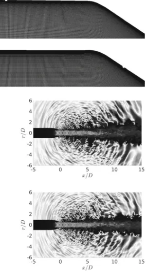
In order to trigger turbulence in the jet boundary-layer, a geometric step is added in the nozzle, as in the work of Vuillot et al. [11]. The height of the step is 0.4mm and its axial length is 1mm. Two positions of the step are tested, in the straight section and in the converging section of the nozzle, respectively. The two simulations will be referred to as case 1 and case 2. Side views of the meshes are provided in Figs.1and2. A simulation without step is also conducted, and will be referred to as the baseline case. It is worth noting that the step should be placed in the nozzle, in the low Mach number flow region, in order to avoid compressibility effects, like the appearance of a shock at the position of the step.

Fig. 1 Case 1: step in the

straight section of the nozzle

Fig. 2 Case 2: step in the

converging section of the nozzle

Fig. 3 Baseline case: Mach

number distribution and near-field pressure fluctuations. The Mach number ranges from 0.25 to 2.5 and the fluctuating pressure from−1000 to 1000 Pa

Fig. 4 Case 2: Mach number

distribution and near-field pressure fluctuations. The Mach number ranges from 0.25 to 2.5 and the fluctuating pressure from −1000 to 1000 Pa

4

Aerodynamic Results

Figures3 and4 display the Mach number distribution and the near-field acoustic waves in a mid-longitudinal plane for the baseline case and for case 2.

The double-diamond pattern of the shock cell structure, observed experimen-tally [6], is visible in the aerodynamic field in both cases. In the near acoustic field, the classical components of supersonic jet noise can be identified; the broadband shock associated noise, mixing noise, Mach wave radiation and screech noise [1]. Moreover, the acoustic waves near the nozzle, propagating in the upstream direction and corresponding to screech noise, have a higher amplitude for the baseline case than for case 2.

336 R. Gojon et al. 0 0.25 0.5 0.75 1 1.25 0 0.1 0.2 0 0.25 0.5 0.75 1 1.25 0 0.5 1 0 0.5 1 0 0.5 1 00 0.5 1 0.05 0.1 0.15 0.2 (a) (b) (c) (d)

Fig. 5 Radial profile of mean axial velocity (a, c) and 2-D turbulent kinetic energy (b, d) at a, b x= D and c, d x = 5D; experimental data (bullets) [6], baseline case (black line), case 1 (dashed line) and case 2 (grey line)

The mean axial velocity and the turbulent kinetic energy of the simulations are compared with PIV measurements [6] in Fig.5. As in the experiments, only the two components of velocity in the azimuthal plane considered are used to compute the 2-D turbulent kinetic energy. At x= D, the results of case 2 are in much better agreement with the experimental results than the results of the baseline case and of case 1, which overpredict the mean axial velocity and the turbulent kinetic energy. This overprediction is characteristic for the transition from a laminar boundary layer inside the nozzle to a turbulent jet shear layer [4,5]. At x= 5D, the three simulations give similar results.

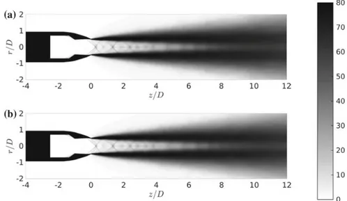
For the baseline case and for case 2, the 2-D mean turbulent kinetic energy is shown in Fig. 6in the plane(z, r). Higher amplitudes are found in the shock cell structure in the baseline case than in case 2. This suggests a stronger motion of the shock cells, which is consistent with a stronger screech mechanism. Moreover, the development of the jet shear layer is slower for case 2 than for the baseline case, yielding a shorter potential core in the latter case. This trend is similar to that observed in subsonic jets [4] as the initial turbulence intensity increases.

Fig. 6 2-D turbulent kinetic energy for the baseline case (a) and case 2 (b). The color scale ranges

from 0 to 80 m.s−1

Fig. 7 Baseline case:

pressure spectra as function of the axial location of the probe and Strouhal number. The color scale ranges from 140 to 155 dB/St

Fig. 8 Case 2: pressure

spectra as functions of the axial location of the probe and Strouhal number. The color scale ranges from 140 to 155 dB/St

5

Acoustic Results

The near-acoustic fields are directly studied from the fluctuating pressure given by the LES. The acoustic spectra obtained at r = 2D, from x = −3D to x = 15D, are plotted in Figs.7and8for the baseline case and case 2, respectively.

338 R. Gojon et al.

Three acoustic components are well visible; the broadband shock associated noise, mixing noise and screech noise. In the upstream region, the screech frequency is observed at St = 0.29, which is in very good agreement with the frequency of St =

0.30 found in experiments [6]. Moreover, the screech amplitude is 5 dB higher

for the baseline case than for case 2, as qualitatively observed in the snapshots of Figs.3and4. In the downstream direction, for x > 10D, the mixing noise is about 3 dB higher for the baseline case than for case 2.

6

Conclusions

Large Eddy Simulations of a round supersonic screeching jet have been performed. In order to reach a turbulent state of the boundary layer at the nozzle exit, a geometrical step is added in the nozzle. With the step in the straight section of the converging-diverging nozzle, no differences with the baseline case are noticed. With the step in the converging section of the nozzle, several differences with respect to the baseline case are observed:

• the development of the jet shear layer is slower

• the overprediction of the turbulent kinetic energy near the nozzle exit is lower • screech noise is 5 dB lower in the near acoustic field

• mixing noise is 3 dB lower in the near acoustic field.

These observations indicate that the geometrical step, under certain circumstances, allow us to simulate more accurately the aerodynamic and acoustic fields of a turbu-lent supersonic jet.

Acknowledgements The computations were performed using HPC resources provided by the

Swedish National Infrastructure for Computing (SNIC) at the PDC center.

References

1. Gojon, R., Gutmark, E., Baier, F. Mihaescu, M.: Temperature effects on the aerodynamic and acoustic fields of a rectangular supersonic jet. AIAA Paper, no. 2017-0002 (2017).https://doi. org/10.2514/6.2017-0002

2. Gojon, R., Gutmark, E., Mihaescu, M.: On the response of a rectangular supersonic jet to a near-field located parallel flat plate. AIAA Paper, no. 2017-3018 (2017).https://doi.org/10. 2514/6.2017-3018

3. Zaman, K.B.M.Q.: Effect of initial boundary-layer state on subsonic jet noise. AIAA J. 50(8), 1784–1795 (2012).https://doi.org/10.2514/1.J051712

4. Bogey, C., Marsden, O., Bailly, C.: Influence of initial turbulence level on the flow and sound fields of a subsonic jet at a diameter-based Reynolds number of 105_{. J. Fluid Mech. 701,}

352–385 (2012).https://doi.org/10.1017/jfm.2012.162

5. Brés, G.A., Ham, F.E., Nichols, J.W., Lele, S.K.: Nozzle wall modeling in unstructured large eddy simulations for hot supersonic jet predictions, AIAA paper, no. 2013-2142 (2013).https:// doi.org/10.2514/6.2013-2142

6. Cuppoletti, D.R., Gutmark, E.: Fluidic injection on a supersonic jet at various Mach numbers. AIAA J. 52(2), 293–306 (2014).https://doi.org/10.2514/1.J010000

7. Eliasson, P.: EDGE: A Navier-Stokes solver for unstructured grids. FOI (2001)

8. Bogey, C., Bailly, C.: Decrease of the effective Reynolds number with eddy-viscosity subgrid-scale modeling. AIAA J. 43(2), 437–439 (2005).https://doi.org/10.2514/1.10665

9. Bogey, C., Bailly, C.: Large eddy simulations of transitional round jets: influence of the Reynolds number on flow development and energy dissipation. Phys. Fluids 50(8), 065101 (2006).https://doi.org/10.1063/1.2204060

10. Kremer, F., Bogey, C.: Large-eddy simulation of turbulent channel flow using relaxation filter-ing: resolution requirement and Reynolds number effects. Comput. Fluids 116, 17–28 (2015).

https://doi.org/10.1016/j.compfluid.2015.03.026

11. Vuillot, F., Lupoglazoff, N., Lorteau, M. Cléro, F.: Large eddy simulation of jet noise from unstructured grids with turbulent nozzle boundary layer. AIAA paper, no. 2016-3046 (2016).