Design and Implementation of Wavescope Storage
Manager and Access Scheduler
by
Jeremy Elliot Smith
B.S., Massachusetts Institute of Technology (2009)
Submitted to the Department of Electrical Engineering and Computer
Science
in Partial Fulfillment of the Requirements for the Degree of
Masters of Engineering in Electrical Engineering and Computer
Science
at the Massachusetts Institute of Technology
September 2010
@
2010 Jeremy Elliot Smith. All rights reserved.
ARCHIVES
MASSACHUSETTS INSTITUTE OF TECHNOLOGY
DEC 16 2010
LIBRARIES
The author hereby grants to M.I.T. permission to reproduce and to
distribute publicly paper and electronic copies of this thesis document
in whole and in part in any
Author ...
medium now known or hereafter created.
Departme
ectrical Engineering and Computer Science
September 10, 2010
Certified by.
Lewis Girod
Research Scientist
Thesis Supervisor
Certified by..
...
Samuel Madden
Associate Professor
Thesis Co-Supervisor
Accepted by ... .
Christopher J. Terman
Chairman, Department Committee on Graduate Theses
Design and Implementation of Wavescope Storage Manager
and Access Scheduler
by
Jeremy Elliot Smith
Submitted to the Department of Electrical Engineering and Computer Science on September 10, 2010, in partial fulfillment of the'
requirements for the Degree of
Masters of Engineering in Electrical Engineering and Computer Science
Abstract
In this thesis, I designed, implemented, and analyzed the performance of an optimized storage manager for the Wavescope project. In doing this, I implemented an impor-tation system that converts CENSAM data into a format specific to the processing system and cleans that data from measurement errors and irregularities; designed and implemented a highly efficient bulk-data processing system that is further optimized with a parallel-processor and disk access reorderer; carefully analyzed various meth-ods for accessing the disk and our processing system, resulting in an accurate and predictive system model; and carefully ran a set of different applications to analyze the performance of our processing system. The project involves low-level optimiza-tion of Linux disk I/O and high-level optimizaoptimiza-tions such as parallel-processing. In the end, I created a system that is highly optimized and actually usable by CENSAM and other researchers.
Thesis Supervisor: Lewis Girod Title: Research Scientist
Thesis Supervisor: Samuel Madden Title: Associate Professor
Acknowledgments
I would like to thank Lewis Girod for being incredibly generous and flexible with his time. He has been particularly patient and helpful, and I have been extremely
fortunate to have him as an adviser and teacher.
I would also like to thank Anne Hunter, MIT Course 6 administrator, for her support, care, flexibility, open ear, and guidance.
I am especially thankful for the support, encouragement, and advice provided by my family while I undertook this extremely challenging endeavor. In particular, I'd like to thank my surrogate aunt and uncle, Judy and Howard Spivak, for their gen-erosity and flexibility.
I'd like to thank my good friend Mark Stevens, without whom my MIT experience would have been remarkably different.
My journey to completing this thesis began long before beginning graduate school. I would like to thank those who lent a hand to my younger self at a time when I was far from where I am now. In particular, I'd like to thank my high school math teacher and advisor, Dr. Yale Zussman, and high school science teacher and coach, John Donohue. And my father, Myron, and sister, Amanda, for their remarkable support of and care for me both before and throughout my MIT career.
Lastly, I would like to thank my late mother, Randi Jill Preman Smith, for helping to instill in me a seemingly impossible dream and for supporting me along my long journey to achieving it.
This work was supported primarily by the CSR Program of the National Science Foundation under Award Number CNS-0720079.
Contents
1 Introduction 17
1.1 Goals of the Project . . . . 19
1.2 Related Work . . . . 20
2 High Level System Design 23 2.1 O verview . . . . 23
2.2 Key Design Considerations . . . . 23
2.3 D ata m odel . . . . 25
2.3.1 Signal . . . . 25
2.3.2 Gap and Discontinuity . . . . 26
2.3.3 Tim ebase . . . . 27
2.3.4 Time and Range . . . . 28
2.4 Importing Data . . . . 29
2.5 Processing System . . . . 29
3 Design and Implementation of the Importer 31 3.1 CENSAM Data Files . . . . 31
3.2 Import Algorithm . . . . 33
3.2.1 Gap Detection and Compensation . . . . 34
3.3 Intermediate Data format . . . . 38
3.4 M etadata . . . . 39
3.5 T im ebases . . . . 40 5
4 Design and Implementation of the Processing System 4.1 Initialization Process ...
4.2 Signal API ...
4.2.1 Signal class . . . . 4.2.2 Timebase . . . . 4.2.3 Time and Range class . . . . 4.3 csignal Module . . . . 4.3.1 Decision to Use Python . . . . 4.3.2 C Python API . . . . 4.3.3 Numpy Arrays . . . . 4.3.4 csignal API . . . . 4.3.5 Auxiliary Functionality . . . . 4.4 Disk I/O and Signal Implementations
4.4.1 Key Design Decisions . . . . . 4.4.2 Signal Versions . . . . 4.5 Access Scheduler and Multiprocessor
4.5.1 A PI . . . . 4.5.2 Optimizations . . . . 4.5.3 Data Structures . . . . 4.5.4 Preprocessing Stage . . . . 4.5.5 Preexecution Stage . . . . 4.5.6 Execution Stage . . . . 4.5.7 Algorithm Summary . . . . . 5 Experimental Setup and Performance 5.1 Test Platform . . . . 5.1.1 System Specifications . . . . . 5.1.2 Caching and Low Level I/O . 5.2 Measurement Methodology . . . . .. 5.2.1 Profiling . . . . 6 . . . . . . . . . . . . . . . . . . . . . . . . . . . . . . . . . . . . . . . . . . . . . . . . . . . . . . . . . . . . . . . . . . . . . . . . . . . . . . . . . . . . . . . . Measurement . . . . . . . . . . . . . . . . . . . . 75 75 76 77 79 79
5.2.2 Tools . . . . 5.3 Baseline Measurements of Platform . . . . 5.3.1 Scan Summarize Application . . . . 5.3.2 Scan Summarize Results . . . . 5.3.3 Results Discussion . . . . 5.3.4 Deriving Page Fault and Reclaim Costs . 6 Trial Application Performance
6.1 Signal Implementation Performance . . . . . 6.1.1 Implementations' Scan Summarize Res 6.1.2 Scan Summarize under Different Size I 6.2 ASM Multiprocessing Performance with Wind 6.2.1 Windowed FFT Application . . . . . 6.2.2 6.2.3 6.2.4 6.2.5 6.3 ASM 6.3.1 6.3.2 6.3.3 6.3.4 6.3.5 6.4 ASM 6.4.1 6.4.2 6.4.3 6.4.4 C++ Version Results . . . . Python Version Results . . . . Single Worker ASM Results . . . . . ASM Speedup . . . . Reordering performance with Backward,
Backwards Scanner Application . . . C++ Version Results . . . . Python Version Results . . . . Single Worker ASM Results . . . . . ASM Speedup . . . . Net Performance with FFT Adding . . FFT Adder Application . . . .
Theoretical Performance Model . . .
Single Worker ASM Results . . . . . ASM Speedup . . . . 7 Conclusions 7.1 Contributions . . . . 95 . . . . 96 ults . . . . 96 nputs . . . . 96 owed FFT . . . . 97 . . . . 98 . . . . 99 . . . . 100 . . . . 100 . . . . 100 s Scan Summarize . . . 102 . . . . 102 . . . . 103 . . . . 104 . . . . 104 . . . . 105 . . . . 106 . . . . 107 . . . . 107 . . . . 109 . . . . 109 111 112 . . . . 80 . . . . 81 . . . . 81 . . . . 83 . . . . 85 . . . . 87
List of Figures
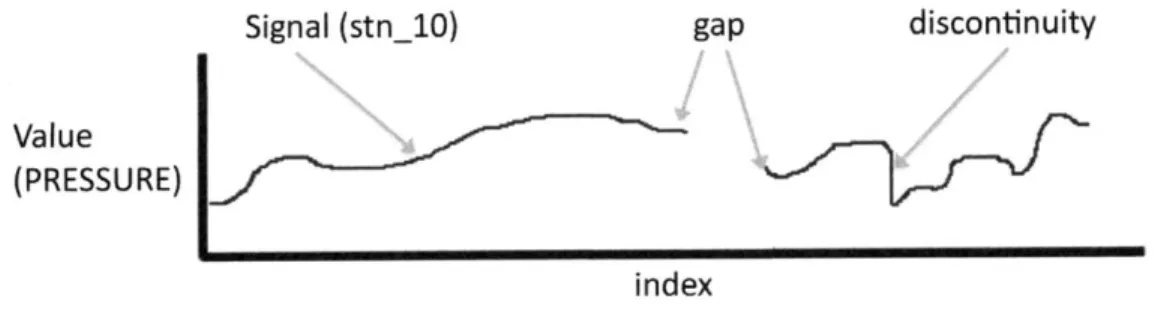
2-1 Overall design of the entire storage management system. . . . . 24 2-2 Diagram of many data model items. The entire red line, a 1-dimensional
vector of points, represents the Signal, which is named stn_10 here. "index" is the Timebase associated with the signal. A gap and dis-continuity are shown. The gap represents a break in the signal where values weren't reported while the discontinuity is an irregularity in the signal (in this case, a drop). The signal value is not explicitly rep-resented. Generally, our signals have been representing the pressure recordings of a CENSAM pipeline station. . . . . 26 2-3 Diagram of Timebase graph demonstrating how Timebases allow for
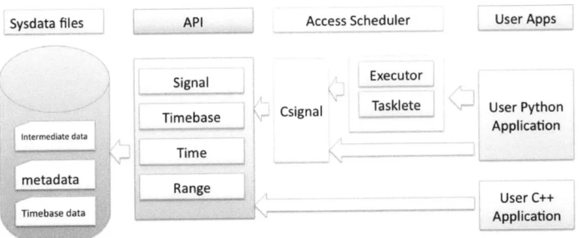
powerful and easy conversion. Each node represents a Timebase and each edge represents a TimebaseMetric. The green edges are Empirical TimebaseMetrics, as the mapping is a list of points from data. The purple edge is Derived, as a linear relationship exists between Seconds and kiloH z. . . . . 27 2-4 Diagram of the entire Processing System. The API provides an
ab-straction for accessing the sysdata files, which the Importer created. The Access Scheduler uses the API to expose functionality to Python. The csignal module serves as the wrapper between the C++ API and the Python world. End-users have the option of developing applica-tions in Python or C++. Python users have the additional benefit of being able to use the Access Scheduler to boost their application's perform ance. . . . . 30
3-1 Diagram of the behavior of the data importer. It takes a set of raw sig-nal files as input and produces a group of files designed for our system. Three files are created: the Intermediate Data file, the metadata file, and the Timebase file. The Intermediate data file contains the actually signal value data. The metadata file contains information associated with the signal. The Timebase file contains an Empirical Timebase providing a conversion between the signal's Timebase and Seconds. . 32
4-1 Diagram of how the Access Scheduler and Multiprocessor interfaces with the rest of the Processing System. The ASM is comprised of the Executor and Tasklete Python classes. Both classes are exposed to the end user. To run the ASM, the user wraps their desired functionality in Taskletes and feed those Taskletes to the Executor. The user uses the Csignal API in combination with the Executor and Taskletes to run the A SM . . . . 61
4-2 Diagram of the ASM dataflow for the FFT Adder Application. Rect-angles represent Taskletes and ovals represent Signals. Here, Tasklete 1 reads in a segment of Signal A, FFTs that segment, and writes the FFT results out to Buffer A. Tasklete 2 does the same with a portion of Signal 2 and Buffer B. Tasklete 3 reads in these segments of Buffer A and B, adds them, and writes the sum to the Output Signal. Tasklete 3 has dependencies on Tasklete 1 and 2 and will not run until they have com pleted. . . . . 62
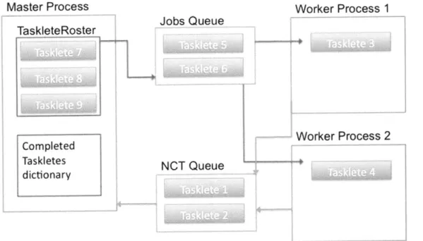
4-3 Diagram of the primary ASM data structures and their interaction. The Master process has Taskletes ordered to optimize performance in the TaskleteRoster. A certain amount of these are added to the Jobs Queue. The Worker Processes pop Taskletes off the Jobs Queue, execute these Taskletes, and then place the completed Tasklete IDs on the Newly Completed Taskletes Queue. The Master periodically pops all Taskletes off this queue and adds the Tasklete IDs to the completedTaskletes Dictionary. . . . . 67 5-1 Diagram of the behavior of our system's I/O. There are several layers
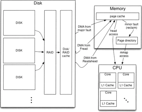
of caching: disk/RAID caching, memory page caching, and individual caches on the CPU cores. Direct Memory Access from either a major page fault, fread, or readahead trigger data to be read from the disk into the page cache. This only happens if the requested page is not already cached. Fread will read directly out of the page cache, while mmap triggers reclaims. Minor faults, or reclaims, cause pages to get
placed into the page directory, from which mmap directly reads. . . 78
6-1 Plot of Signal implementation runs of Scan Summarize with different loads. X-axis represents data processed in Megabytes Y-axis is Total Loop time in seconds. The theoretical maximum is computed using our systems' maximum throughput. . . . . 98 6-2 Plot of ASM speedup for Windowed FFT application. X-axis
repre-sents number of workers. Y-axis is speedup using the base value of 1 w orker. . . . . 102 6-3 Plot of ASM speedup for Backwards scan with reordering. X-axis
represents number of workers. Y-axis is speedup using the base value of 1 worker. Naturally, we don't see an improvement with more workers, as we are I/O bound. . . . . 106 6-4 Plot of ASM speedup for FFT Adder application. X-axis represents
List of Tables
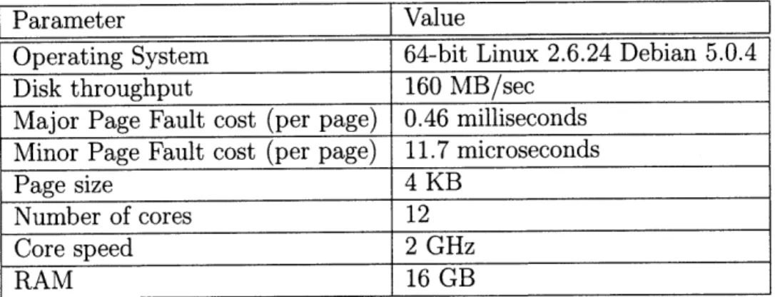
5.1 Key system specifications, measurements, and parameters. . . . . 76
5.2 Summary results from profiling tests of different implementations of Scan Summarize. There are 3 trials per version, all of which are fairly close in value. Times listed in seconds. . . . . 84
5.3 Summary page fault and reclaim results from tests of different im-plementations of Scan Summarize. Multiple trials were run but results were identical between trials. The data load is 3.67 GB, or more specif-ically 3,947,364,352 bytes. This is exactly 963712 pages. . . . . 85
5.4 Derived System Parameters. . . . . 93
6.1 Summary results from profiling tests of different implementations of Scan Summarize. There are 3 trials per version, all of which are fairly close in value. Times listed in seconds. For a more thorough breakdown of these tests, see Table 5.2. . . . . 97
6.2 Windowed FFT C++, Linear Python, and single worker ASM runs. Total time includes initialization and startup (loading signal sysdata, importing packages, etc.). Total Loop is the cost of reading signal data and processing and has no applicable value for single worker ASM. Times listed in seconds. . . . . 99
6.3 ASM FFT with 1 worker results. Total time includes initialization and startup (loading signal sysdata, importing packages, etc.). Preprocess-ing is the time for the PreprocessPreprocess-ing stage of the ASM (creatPreprocess-ing the Taskletes, etc.), as described in Section 4.5.4. Execution is the time actually running the ASM, though technically includes both the Pre-execution (Section 4.5.5) and the Execution Stages (Section 4.5.6). For reference, these totals are compared to serial implementations in Table 6.2. Times listed in seconds. . . . . 101 6.4 C++ scan forward, C++ scan backwards, and Python Scan Backwards
test results. The C++ Scan Forwards results were first displayed in Table 5.2. Slowdown is relative to median C++ Scan Forwards case. Times listed in seconds. . . . . 103 6.5 ASM with one worker scan backwards without ordering. Times listed
in seconds. ... ... 104 6.6 ASM with one worker scan backwards with ordering. Times listed in
seconds. ... ... 104 6.7 Single worker ASM results for the FFT Adder application. . . . . 109
List of Listing
3.1 The algorithm for importing data into the system for processing. . . 34
3.2 The algorithm for detecting a gap or discontinuity in data . . . . 37
5.1 Profiling code using the Time Stamp Counter register. . . . . 80
5.2 The linux script we used to clear the memory caches. . . . . 81
Chapter 1
Introduction
Many scientific research projects involve processing and analyzing large quantities of data. However, as the size and complexity of the data sets increase, managing these data sets becomes outside the scope of many analysis tools. When dealing with such large amount of data, fundamental system constraints that usually may be ignored become relevant. RAM is limited in size; many common and useful analysis appli-cations (eg Matlab) have either an intrinsic or practical size limitation on imports; seeking on a hard disk is time-intensive; and so forth. The Wavescope, an ongo-ing project worked on by Dr. Girod and Prof. Madden at MIT CSAIL, provides a platform for building distributed systems to capture and process high rate sensor data.
This MEng project involved designing, implementing, and testing a system that provides a powerful yet relatively intuitive and simple interface for accessing, manip-ulating, and analyzing large quantities of data. As such, our work has taken all of the aforementioned constraints into consideration. In particular, we have carefully designed, implemented, and evaluated a storage manager and processing system for the CENSAM Pipeline project [7] ; the pipeline's distributed sensor network has been collecting terabytes of data that our system allows scientists and engineers to analyze and process.
The sensor network, rightfully focused on reliably recording accurate pressure data from the pipeline , stores the data in a series of timestamped binary files that is cum-bersome to index. Further, the data is often inconsistent, riddled with reflections of changes to the recording system, errors and bugs with that system, and the same noise that is to be expected in any such sophisticated sensor system. With this in mind, our first task, was to devise a process for cleaning this data and convert it to a format more conducive to analysis and processing.
The next component involved the creation of the actual processing system and its API. As can be expected when dealing with such large amount of data, our primary design challenge was performance. With this in mind, our work involved developing our own internal data format, implementing and evaluating several different versions that each have different low-level I/O procedures, and utilizing the full capacity of the system's resources through multiprocessing and the creation of an intelligent access scheduling system.
Finally, we rigorously experimented to measure the different implementations' per-formances and determine which implementations are best and why this is the case. In doing this, we painstakingly analyzed our system and developed a solid grasp on its low-level I/O behavior and performance. The result is an accurate system model for each of the different implementations of our processing system. Next, we analyzed many variations, implementations, and pieces of our system to bettervn understand its behavior and optimize overall performance.
Despite the specificity of our system around the CENSAM project, our results are fairly generic and, we believe, widely applicable to many bulk-data systems.
1.1
Goals of the Project
Our overall project had specific criteria and high-level requirements that guided our work.
1. Handling large datasets
The most important requirement is that the system is able to store and provide efficient access to large quantities of data for both streaming and random access patterns. The exact nature of what is meant by provide efficient access was not well defined before the project's start; but we were aware that storage should be done in such a way that information can be accessed more quickly than the naive approach of saving all files to disk and seeking through the data. We expected that some form of caching and indexing would come into play.
2. Handling metadata
Our project needed to be able to accept metadata along with data and provide a means of correlating metadata with the main data set. The system needed to be robust yet flexible as the possibilities for what metadata can describe are limitless. In the obvious use case, the metadata indicates, among other things, the start times of the set of files recorded into by the sensor system and each files' length. The program must use this metadata to piece together the differ-ent data files for continuous analysis.
3. Handling discontinuous data with varying time-base
The sensor network did not always run with precise timing or a perfectly stable sampling rate, the only precise time measurements made were at the start of a data file recording, and many sensors were down or failed for a period of time. Thus, the software must be able to intelligently reason about the input in order to handle discontinuities and inconsistencies like these. There are conceivable solutions to these problems. For instance, for missing data, our system could
draw a best-fit line between the two adjacent time-marked points, and use that line to interpolate a given point's absolute time.
4. Present views to the user/application developer
End-user specified views must be supported. One could imagine the use case of needing to decimate data and achieving this by presenting data in a decimated view. These views must not only be presentable to users they should be ac-cessible programmatically. This allows for more complicated analysis through another application.
5. Provide programmatic interface
The project should provide interfaces for more complicated data analysis than that provided in views. There are many options for satisfying this requirement:
a Matlab plugin, the WaveScope language WaveScript, or by simply allowing users to write C-code (or code in some other programming language).
1.2
Related Work
A variety of work in the field of signal processing and signal storage management has been done.
Developed at CSAIL by Prof. Madden and Dr. Girod (among others), WaveScope provides a platform for building distributed sensing systems to capture and pro-cess signals. The technology consists of several innovative functionalities. First, WaveScope introduces a signal segment data type, which provide efficient operation on data and an efficient means to pass signal data through a dataflow graph. Sec-ond, it provides end-users with a novel programming language that minimizes data conversion between applications/databases thereby reducing end-user programming
effort and boosting performance [3]. Lastly, executed queries can be distributed across many nodes; this is quite useful as many of WaveScopes target applications are in-herently distributed due to their sensor networks [4] [2].
Current work in Wavescope has been designed for streaming and memory pro-cessing without addressing storage issues. Our work on a WaveScope-compatible storage manager enables the WaveScope system to efficiently process input streams from stored data, run queries over that data, and store the results.
The TimeSeries DataBlade database system was designed to handle large-quantities of time-related data [8]. It can be paired with auxiliary technology to handle huge volumes of streaming, real-time data. The database system itself, however, has a SQL-like interface not suited for the type of analysis that motivates our project. To implement signal processing queries of the type supported by WaveScope, one would need to expose a programmatic DataBlade API.
Borealis is a distributed stream processing engine that provides functionality for dynamic revision of query results, dynamic query modification, and flexible opti-mizations [9]. Like WaveScope, Borealis is focused on streaming data and does not currently have a processing specialized storage manager to support high performance access to stored signals. Our work might be applicable to Borealis with modification, to enable Borealis VMS to run efficient queries over stored data.
Chapter 2
High Level System Design
2.1
Overview
The storage manager and processing system is comprised of several distinct compo-nents and conceptual abstractions. We begin this chapter by a discussion of the key principles we kept in mind when designing our system. Next, we go on to discuss that to manage the complexity of data we are processing, we have come up with a data model that provides nomenclature and abstraction. After that, we discuss the design of the process of copying the data files produced by the sensor reading system into our internal system format, known as importing. Lastly, we give a high-level overview of the actual processing system, which provides an API for accessing and analyzing the data and also a system for parallelizing and optimizing analysis algorithms.
2.2
Key Design Considerations
The fact that scientists and engineers working on the CENSAM project are dependent upon using this project serves as the biggest underlying driving force for our design. Resulting from this, we have had five main design considerations.
1. Correctness
CENSAM files Import Process Sysdata files Init process API
Signal Timebase
Intermediate data Time
Range
metadata
Timebase data Private Implementation:
TimebaseNode TimebaseMetric Metadata (JSON)
Figure 2-1: Overall design of the entire storage management system.
research beyond the lifetime of our work, it is important that the system works as claimed and produces accurate results. Given this requirement, we have operated with the understanding that correctness is not absolute and there are trade-offs to be made. While we have paid careful attention to producing accurate results, we have also worked hard to keep the project in scope. For instance, some of our data cleaning operations during the import phase could probably be improved further, but instead of exerting too much effort on this, we chose to focus on other areas more in-line with the big picture of our project.
2. Performance
Perhaps the largest constraint for which we optimized, system performance and speed played a crucial role in our design. As stated in our first high-level goal, we strive to access large quantities of data faster and more conveniently than using the ad-hoc format originally chosen for CENSAM data. We are not concerned with system start-up, preprocessing, import, or shutdown performance, and are concerned with steady state data processing operations.
3. Maintainability
As is typical of research code, the implementation work on this project has a relatively short lifespan. In order to increase the likelihood that this system has continued use throughout the longer term CENSAM project (and perhaps beyond), it has been important to ensure the system and code is easily main-tainable. As a corollary, it is important that others can easily understand the system and its code-base so others can maintain it.
4. Extensibility
It is important that the system is easily extendible to match the potentially changing requirements and nature of the CENSAM project. Further, while our primary driving focus has been CENSAM, we have aimed to create a system modular enough that it can be used in other projects and environments with relatively little difficultly.
5. Usability
While our primary user-base is inherently technical, we have kept in mind the importance of keeping our system fairly easy to use. Maintaining a clean and straight-forward API and installation procedure along with the use of preexist-ing tools like Python NumPy, will improve our system's adoption rate and the ease with which others can maintain and extend it.
2.3
Data model
Our data model is comprised of several concepts: a signal, timebase, gap, discontinu-ity, time, and range.
2.3.1
Signal
A signal is a vector of 1-dimensional points and associated metadata, representing a continuous sampling process. In essence, a signal is comprised of a series of
measure-Signal (stn_10) gap Value
(PRESSURE)
index
Figure 2-2: Diagram of many data model items. The entire red line, a 1-dimensional vector of points, represents the Signal, which is named stn-10 here. "index" is the Timebase associated with the signal. A gap and discontinuity are shown. The gap represents a break in the signal where values weren't reported while the discontinuity is an irregularity in the signal (in this case, a drop). The signal value is not explicitly represented. Generally, our signals have been representing the pressure recordings of
a CENSAM pipeline station.
ments and at what time those values occurred. The metadata includes information about the signal such as the name of the signal, the length of the signal, and the sig-nals timebase and gaps which are further explained below. A signal may be read-only or writable and can persist across system restarts. There is a "buffer" subtype, which does not persist between system restarts and is used as programmatic scratch space.
2.3.2
Gap and Discontinuity
A gap is a consecutive series of samples in a Signal that have no value. Conceptu-ally, a gap can occur any time a CENSAM sensor has downtime due to a restart, shutdown, or network outage; a gap can also result from a hardware or software bug that causes data loss. In all of these cases, the time between consecutive samples will not match the predicted time (which is calculated through the station sampling rate).
A discontinuity occurs when there is a changes in values between consecutive samples is far greater than is reasonable or expected or when a future sample (by sample number) has an older timestamp. These typically show up as big spikes or drops in a signal value. timebase plot. Discontinuities can occur if there is a hardware
or software error that causes dropped samples or erratic values, or when timestamps are recorded before GPS lock has been established.
2.3.3
Timebase
Stn; 10 & Seconds Metric
Seconds KiIoHz
%Metric
St a111 Met ic Stn 10 & Stn 11 Metric
Figure 2-3: Diagram of Timebase graph demonstrating how Timebases allow for pow-erful and easy conversion. Each node represents a Timebase and each edge represents a TimebaseMetric. The green edges are Empirical TimebaseMetrics, as the mapping is a list of points from data. The purple edge is Derived, as a linear relationship exists between Seconds and kiloHz.
The timebase abstraction represents the time dimension of a signal: a handle for the unit of time exhibited on a signal plot's x-axis. Thus, a timebase conceptually represents a unit of time. Seconds, CPU clock cycles, and the sample count of station 10 are representations of time and are therefore valid Timebases. Every signal has a single timebase associated with it in its metadata. [2]
We decided to abstract away the time-value of a signal because a common use-case is to make comparisons between signals that have different timebases, but that have some empirical conversion relationship. For instance, a CENSAM sensor station by default has a timebase unique for that station; that is, the sample clock at a station is locally linear, thus the sample count is the most precise way to annotate the time at which a sample was captured. Each station, therefore, has its own mapping of
indices to seconds based in GPS.
Thus, in order to compare two separate CENSAM sensor station readings (which CENSAM researchers would want to do for such things as detecting a leak), we can convert a station's timebase to that of another station's by constructing a relational graph of all of the timebases. In this example, a station can be compared to another by first converting to Seconds and then to that second timebase. Further, since there is a relationship between Seconds and other values, we can readily remap a Signal onto other time axes.
These relationships can be defined using a graph model. Each node on the graph is a Timebase and each edge is a TimebaseMetric. Thus, a TimebaseMetric represents a relationship between two Timebases. There are two kinds of relationships: empirical and derived. An empirical metric is a mapping defined by an explicit correspondence of values between two Timebases - that is, list of pairs of corresponding points, e.g. station 10 sample number and second. A derived metric is a linear equation relating two Timebases. Derived metrics are used to perform time unit conversions.
2.3.4
Time and Range
As with any system dealing with signal processing, it is natural that our system have a way of representing a single point in time. We created a separate Time object to encapsulate this concept. To represent a point in time we use a pair of a double and a Timebase. A Time can be thought of as a value with its unit, as in 3 seconds, or the 3rd station 10 sample. By explicitly including the time unit with the value, we can easily convert a Time point in one Timebase to that in another and avoid confusing in which Timebase a value is measured. A range is simply a pair of Times
2.4
Importing Data
The system imports data into a special system format before that data can be used. Since this is a one-time process, we don't focus on the performance of the import process. Given the large variation in existing data representations, we did not at-tempt to design a universal import API. Rather, we constructed a CENSAM-specific importer. However, much of the techniques and discussion regarding our CENSAM importer can be easily applied to other importers.
For a single signal import, the system outputs 3 system data files: the intermedi-ate data file, the metadata file, and the timebase file. With our CENSAM example, we have create a signal for every station, so each station produces 3 files. The import process also detects gaps and discontinuities to place the data into a consistent and coherent timebase.
Once any particular data set is converted to the system data format, the pro-cessing system will work fine with it. That is, the application-specific details of the import system is encapsulated away from the rest of the system and once a data-specific importer is written the rest of the system will perform as well as it does with the CENSAM data.
2.5
Processing System
The Processing System is the primary design and implementation component of the Storage Manager System. As such, significant design thought and effort went into its creation.
The Processing System is comprised of many components. The previously dis-cussed Sysdata files are the datastore for signals and all persistent information.
Writ-ten in C++, the API exposes a simple yet powerful interface for creating, accessing, and modifying, Sysdata files. Since the primary abstract data type in the API is the Signal, we generally refer to the API as the Signal API. The csignal module is a wrapper over the Signal API that exposes its functionality to Python. The primary end-client of the csignal wrapper is the Access Scheduler, a Python module written to optimize the runtime of users' queries, although csignal is by no means encapsulated by the Access Scheduler.
Sysdata files API Access Scheduler User Apps
Executor
Timebase Csignal Taskete User Python
Intermediate data Application
Time metadata
User C++
Timebase data -0 -- *-*--- - - - Applicationpcto
Figure 2-4: Diagram of the entire Processing System. The API provides an abstrac-tion for accessing the sysdata files, which the Importer created. The Access Scheduler uses the API to expose functionality to Python. The csignal module serves as the wrapper between the C++ API and the Python world. End-users have the option of developing applications in Python or C++. Python users have the additional benefit of being able to use the Access Scheduler to boost their application's performance.
In the end, we are left with a powerful, high-performance system that can quickly perform complicated operations on the huge amount of data that is stored in the system. The system in flexible in that users can choose to develop in either Python or C++. Further, we were able to design our Python modules in such a way as to ensure there is not really a significant performance hit. And if a user does develop in Python, they have the benefit of having the Processing System optimize their perfor-mance.
Chapter 3
Design and Implementation of the
Importer
While the Importer is not the main focus of our work, it is an essential component to our system. As the majority of our work centered around designing, implementing and optimizing the processing system, a good amount of thought went into designing an optimizing format in which the processing system's data is stored. Naturally, the design of this format impacts the Importer's design considerations and constraints and import algorithm. Further, the data must be massaged and cleaned up the data so that it is in a state ready for practical analysis. One notable difference in require-ments for the Importer is that since the import process only occurs once, we were not concerned with optimizing its performance.
3.1
CENSAM Data Files
We worked with the CENSAM pressure sensor data set. Although the importer we made is custom to this particular dataset, the principles apply more generally.
There are approximately 15 stations in the dataset. While the present and valid data for each station is not consistent among stations, each station has about a years'
Concatenation of all CENSAM
ntermediate data station files into a single raw data
file spaced appropriately for gaps
Station 10 JSOIN file with associated info
Ftie 0 metadata (name, station id, number of
samples, last sample index, list of gaps and discontinuities, etc.)
Timebase data Contains Timebase mappings (ie
-series of index points to seconds).
Figure 3-1: Diagram of the behavior of the data importer. It takes a set of raw signal files as input and produces a group of files designed for our system. Three files are created: the Intermediate Data file, the metadata file, and the Timebase file. The Intermediate data file contains the actually signal value data. The metadata file con-tains information associated with the signal. The Timebase file concon-tains an Empirical Timebase providing a conversion between the signal's Timebase and Seconds.
worth of days in pressure data. Many of the stations have other sensor data (temper-ature, battery, etc.), We worked primarily with station 10 pressure data, which has 372 days present in total.
The data is organized into a directory hierarchy of station, year, day, and lastly sensor-type. That sensor-type directory contains all the data files for that given day and sensor-type. This scheme was a design decision of the sensor system and from our perspective was a preexisting choice.
The pressure files are 120,000-byte raw-data files where each 2-byte value is an individual sample stored consecutively. Thus, each file contains 60,000 samples, rep-resenting a 30-second sampling segment. The system has a nominal sampling rate of 2 kHz. These values are consistent since (60, 000)/(2kHz) = 30 secs. On a day when the sensor does not malfunction and produces all the data files, there are 2,880 files
We import these data files into the Intermediate Data Format, one sequential sparse binary, which is discussed in detail in Section 3.3. In this format, station 10's data amounts to about 60 Gigs. Note that because our imported system data file is sparse, it should be more compact than CENSAM Data Files. Still, their size should not be more than a factor of 2 greater (in fact, assuming perfect recording, the CEN-SAM files would be 2, 880 * 372 * 60, 000 *2 bytes 120 GB, which is about twice the size of our imported data.
Each file is named with the station name and a timestamp of the first sample with second accuracy. From these stamps, we can verify that each file contains 30 seconds of data. More importantly, this characteristic will become crucial for gap and discontinuity detection.
3.2
Import Algorithm
The import algorithm scans all of a signal's disparate files sequentially and produces the appropriate system data files in a consistent and accessible format. While iterat-ing through the original signal files, the algorithm checks for gaps and discontinuities.
function importStation(stnname) {
Create EmpiricalTimebaseMetric between stnname and Seconds Create a Metadata file for stn-name
Create an IntermediateData file for stnname Sort all files for stn-name
Iterate through sorted file list:
Compute Exponential Windowed Moving Average with prev file If there was a gap or discontinuity:
Mark this in Metadata file and
Increment/decrease index // ensures the file is sparse
Write file data to iData file
Write empirical mapping to TimebaseMetric file
Write number samples, end index, etc. to Metadata file
}
Listing 3.1: The algorithm for importing data into the system for processing.
3.2.1
Gap Detection and Compensation
Although our import procedure will only detect gaps and discontinuities between file boundaries and not on samples inside files, this is a limitation of the original data format. This allows us to avoid the painful process of iterating through every entry in every file and performing more complicated data massaging and detection algo-rithms. Further, we have been focusing on the huge-data cases; small glitches within 30-second files will be negligible when dealing with days and perhaps months worth of data.
Key to our gap detection and compensation algorithm is prediction of the sampling frequency. While, we know the CENSAM sensors' sampling frequency is set to a nominal value of 2 kHz and is locally linear, the sensor system's clock frequency will drift over time such that the sampling does not occur precisely at 2 kHz. In addition, each timestamp will have some measurement error associated with it.
Despite the variance in actual sampling frequency, the file timestamps we are given are from GPS and therefore are accurate despite some degree of imprecision from sampling error. Thus, using the timestamps and number of samples in a file, we can predict the average sampling frequency over the file. Given that we expect slippage to be minimal, we can use this computed value as a better approximation of local frequency. In fact, we can combine this value with neighboring files' own computed frequencies to obtain an even better approximation.
Having a good approximation of the local frequency is necessary when dealing with gaps for two reasons. First, given that we have reliable values for only the start of each file and the number of samples in each file, we can use the approximate fre-quency to predict the time of the last sample in a file. Given that we expect each file to be adjacent, if there is a sufficient difference between the end sample timestamp of one file and the begin sample timestamp of the next file, we detect a gap. Second, having a good local frequency approximation enables the algorithm, after detecting a gap, to extrapolate how many samples large that gap is and thereby compensate for the gap.
Implementation
As discussed previously, because gap detection is coupled with import, the gap detec-tion algorithm is embedded within the file import code. Our algorithm begins with initialization of constants. In particular, the currentFrequency initializes its estimate with what we were told was the actual polling frequency.
In the standard import procedure, we iterate over all the files. We compare the difference between the timestamp of the beginning of the current file with the pro-jected last timestamp of the previous file. This difference conceptually corresponds to the time between files: if it is large, we have a gap and if it is negative, we have
a discontinuity. We allow for timestamp impression with the GAPSLIP constant (which is set to 0.075 seconds). A discontinuity has a negative difference.
Once an irregularity detected, we estimate its size in samples by multiplying the previously found time distance between files with the currently estimated polling fre-quency. To compensate for the irregularity, we increment the running index (which is used in normal import code to keep track of the current index of whatever is being imported). We then record the gap or discontinuity in metadata.
At this point, we run the normal import code. This happens regardless of whether or not an irregularity was detected. If we have compensated for a gap or discontinuity, the effects from that impact normal import code through the change in size of the
running index.
As a final step, the algorithm must update its state. First, it estimates the end timestamp of the end of the file by dividing the number of samples by the current frequency and adding that to the beginning timestamp (recall that this value is used when detecting irregularities at the start of the loop).
In what is perhaps seemingly the most complicated step, the algorithm uses pre-viously computed values to update the current approximate frequency. First, we compute the average frequency for the given file by dividing the files' sample count (in addition to any samples it may have gained or lost from gaps and discontinu-ities) by the difference between the previous files' start timestamp and this files' start timestamp. This is the average frequency between files including irregularities. Then, we combine this with the current running average frequency through the use of an Exponentially Weighted Moving Average. The result is a more precise local frequency.
1 currentFreq= 2000.033
2 prev-file-endtimestamp = 0
3 lastfiletimestamp = 0
4 for file in sortedListOfImportFiles:
5 // detect gap and discontinuities
6 double gapSpace = file.starttimestamp
-7 prevfile.end-timestamp
8 bool wasGap = gapSpace > GAPSLIP
9 bool wasDiscontinuity = gap Space < 0;
10 if (wasGap || wasDiscontinuity) {
11 double indicesInGap = gapSpace*currentFreq;
12 running-import-index += indicesInGap
13 // save gap in metadata
14 recordgap-ordiscontinuity(index, indicesInGap, file)
15 }
16 // run the import file prcedoure
17 normalImportFileProcedure(running-import-index, file)
18 // approximate timestamp of last file sample
19 double fileSecs = file.num-samples/currentFreq
20 prev.file-end-timestamp = file.starttimestamp + fileSecs
21
22 // update approximate frequency based on what we now know
23 double secsBtwnFileTs = file.starttimestamp
-24 last-file-timestamp
25 double localFreq = (file.samples + gapSpace)/secsBtwnFileTs
26 // update current frequency using EWMA formula
27 currentFreq= alpha*curentFrequency + (1-alpha)*localFreq
28
29 last-file-timestamp = file.starttimestamp
An Exponentially Weighted Moving Average is a moving average where the weight of each future data point decreases exponentially. In doing this, we ensure future changes impact the change in estimated frequency slowly. We define the EWMA
using the formula Ri = R * a + A * (1 - a).
We used the following parameter values:
a = 0.999999,
Ro = 2000.033
3.3
Intermediate Data format
Our Intermediate Data Files contain all signal value data. Each signal has one single IData file. The Intermediate Data file is thus a concatenation of all signal RAW files in sorted order with appropriate spacing for gaps. That is, every samplesize bytes contains a distinct sample or the n sample begins at the n * samplesizeth byte and is
of length samplesize. We chose this format for several reasons.
First, the approach allows for a very simple lookup algorithm, which is
sampleValue(n) = n * samplesize
We use O/S facilities where possible and only invent new ones if needed. Hav-ing a simple algorithm helps with implementation, testHav-ing, and thereby increases the chance of correctness. Further, the algorithm requires very little processing. It also allows for easy debugging.
Second, having contents in a single file optimizes for the use-case of scanning a file. We believe this is a common use case for large signal processing because in order to
understand the data, it often makes sense to summarize large chunks of consecutive data (ie - by taking averages). Further, by the spatial principle of locality, values logically sequential or related are highly likely to be accessed together. Storing data sequentially guarantees that a block on the hard disk will have an ordered list of sequential samples. Since we are using a single file, it is highly likely blocks are also stored sequentially on disk. This in turn, takes advantage of the system's multitude readahead operations (some of which occur at the hardware level, some in the oper-ating system, and some by our specific application).
Third, creating the file is simple and painless with our sequential import algorithm, defined in Figure 3.1. This reduces the possibility of errors and thereby increases cor-rectness.
A benefit of having sequentially-mapped files is that by only writing segments that are used, the file will maintain a consistent time index without consuming the extra space.
3.4
Metadata
Metadata files contain all remaining signal information that is not stored in the In-termediate Data File. This includes information that can be derived from the IData File but is expensive to compute. Fields of the Metadata file include the number of samples in a signal, the end sample index (which is different than the number of samples since samples omitted due to gaps have indices), the signal's nominal rate, and a log of "events" that occurred in the signal.
Currently, the log is used to annotate gaps and discontinuities. A gap contains a starting index, a length, and some debugging information (original file and times-tamp). A discontinuity contains only a index and original file for debugging. We use
this log to track which parts of the IData are valid signal data and which are gaps.
The log is implemented as a sorted list of log events. A log event contains an identifying tag, and any number of custom values (which are dependent upon the log type). This allows for extreme flexibility and extensibility; we can easily add infor-mation about different parts of the signal to the log.
The Metadata files are not intended to hold a huge amount of data. For example, station 10 has 60 IData file, but the Metadata file is only 512KB. Fortunately, this easily fits in memory and we did not have to focus on optimizing its design for per-formance. We chose to implement it in JSON due to the availability of APIs and its readability.
3.5
Timebases
A Timebase file represents an Empirical Timebase Metric between the current signal's indices and seconds. As such, it contains some information about the metric (such as the peer Timebase's nodes) and the type of the Timebase Metric (derived timebases also have Timebase files, but these are never created on import).
To define the relation from one timebase to another, the file contains a list of corresponding points in two timebases. We record one pair of corresponding points for each timestamp defined in the input data (that is, one pair for each file). Since the majority of samples in a signal does not have a direct mapping, it is the responsi-bility of the processing system to interpolate between adjacent corresponding points to estimate a timestamp value for a given sample, and vice versa.
Timebase Metric files are much larger than Metadata files, but are still substan-tially smaller than IData files. Station 10, for instance, has a 32 MB Metadata file.
While this is fairly large, it is still small enough to easily fit into RAM, and we do not consider the scaling impact of timebases on processing system performance. For similar reasons to those discussed in the Metadata section, we also save Timebase files in JSON.
Chapter 4
Design and Implementation of the
Processing System
The design and implementation of the Processing System is the main implementation effort of this work. The system enables efficient processing of very large quantities of data through optimized disk I/O strategies, a usable and flexible API, and a sophis-ticated scheduling and multiprocessing module.
4.1
Initialization Process
Upon system startup, the Processing System goes through an initialization stage where it loads the appropriate Timebase and TimebaseMetrics into memory from Sysdata files. We are not concerned with the performance of this aspect of the system, as we are more focused on the runtime performance of steady state Signal operations. Note that neither Signals nor their metadata are preloaded at this stage; that happens upon specific Signal loading.
4.2
Signal API
The Signal API is intended to provide a powerful yet simple interface for accessing, modifying, and creating Sysdata. It is designed for high-performance behavior with large quantities of data. As such, it is written with a combination of low-level C and C++.
The interface is entirely exposed in C++. Despite the complexity and many mov-ing parts of what the Signal API is abstractmov-ing away, we end up exposmov-ing only a handful of classes that provide sufficient functionality: Signal, Timebase, Time, and Range.
4.2.1
Signal class
The Signal class is the primary abstraction in the Processing System API. It repre-sents a signal, as defined and discussed in Section 2.3.1.
During the design process we experimented with several different implementa-tions of Signal. The differences all centered around low-level disk I/O techniques
and, besides performance, all implementations behave the same. Our strategy was to begin with the simplest implementation and increase complexity of our solution incrementally as warranted by performance gains. See Section 4.4 for a discussion of the different Signal implementations.
Initializing
One can either open a preexisting signal or create a new one. When opening, a signal can be read only or writable; read-only is useful for important signals that should be immutable, ie input data sets.
are created. These are written to disk upon a call to Signal's save method (discussed below). Users have the option of truncating a new signal, in which case, if an old signal exists with an identical name, it will be replaced.
When opening, the Signal loads all metadata into memory, including gaps and discontinuities. As discussed in Section 3.4, Metadata files are inconsequential in size, so we can neglect the cost of loading. Also, as a reminder, we do not attempt to optimize initialization costs since they are one-time costs and are negligible in com-parison to the steady state costs when the system is run over large data sets.
Gaps and discontinuities are then stored in an internal vector data structure. A Gap is represented as a Range, which as explained in 2.3.4 is simply a pair of times.
It may seem as though storing all gaps internally could be a wasteful use of system memory, but we found this not to be true. Given that we only detect gaps between files (see: 3.2.1), in the worst case of 2 years' worth of data with a gap per file, with an unoptimized 300 byte Range implementation, the gaps data structure is still less than half a gigabyte. Storing gap data in memory lowers the cost of iterations over contiguous portions of a signal, which is a common use case.
In general, we've determined that binary searching through gaps lists to be an adequate search strategy. Some speedup could be achieved through implementation of a more complicated gaps data structure, but we leave this to future work.
Buffered Types
Signals can also be "buffered" in the case that they do not need to be saved. Buffered Signals has an Intermediate Data file, but whenever the Signal is garbage collected, the file is deleted. Metadata and Timebase/TimebaseMetrics for the Signal cannot be written out.
Buffered Signals were created due to the need to have temporary space during computation. In particular, certain implementations of Signal use shared memory (discussed later) and Buffered Signals are used in the Scheduler/Optimizer for inter-process communication. We provide a separate factory creation method for making Buffered Signals.
Accessing and Modifying data
The access mechanism for data is a function called ptr(). It accepts a Range and returns a pointer to a contiguous region of RAM containing the corresponding data. Note that ptr() does not guarantee that the data has been paged in from disk (this is implementation dependent). It is the responsibility of the client to call release() in order to appropriately clean up the memory space when the data is no longer used.
Note that since ptr() takes a range as an argument, it is possible to ask for a set of data using Range, defined in a timebase other than the Signal's native timebase. For instance, one could conceive of needing to investigate a leak that seemed to occur at 12:30AM on a given day. Instead of worrying about the station's sample to Sec-ond conversion, one can simply pass pointer a range in the SecSec-onds Timebase with timestamps of midnight and 1AM for the given day.
Ptr 0 requests a read only region of memory; there is a another function writePtr 0 for requesting a writable region. By making each request explicit about which signal sections are writable and which aren't, the implementation is better able to optimize access. For example, if there is additional cost for writable segments, writePtr 0 can implement its own algorithm for the cost unique to writing. There is also an append() operation that extends the size of a signal and adds samples onto the end.
Gap Functionality
The primary use-case for gap data has been to check if a given region contains or over-laps a gap. Thus, we provide the contiguous() procedure which accepts a Range and returns true if no gaps exist in or overlap the end points of the region. The implementation involves binary search algorithm variant of the gap list to find a gap
in violation.
For writable signals, we provide appendGap 0. It is currently not possible to insert a gap into a signal.
Saving
Signal's save ( function is applicable only to writable signals (and, in particular, not Buffered signals). It writes a Signal's metadata and Timebase information to disk. The operation is intended to be used once - after a signal is created or one is modified with the intention of being reused later.
Save ( does not necessarily write out Intermediate Data -that is implementation dependent and typically happens when the data structure is written to.
The Process Manager is not fault-tolerant. That is, if an application is interrupted or crashes, the signal will be irrecoverable; the Metadata and Timebase information will not be saved. Note that it is possible that the Intermediate Data may be intact or partially written, but this information is contextually useless. Fault tolerance can be implemented by logging changes to the data and using a write-ahead discipline, but this was outside the scope of this project.
Auxiliary functions
The API also include several auxiliary functions. Many of these functions manipu-late the Signal Metadata. For a discussion of data contained in a Metadata File, see section 3.4.
sampleCount 0 returns the total number of valid samples (excluding gaps).
endIndex() and startIndex() return the corresponding indices in the Signal's timebase (these return 64-bit integers, not Time objects).
indexOf () accepts a Time or Range in any Timebase and returns either a Time or Range in the signal's Timebase (with its value converted appropriately). This conversion function is a simple wrapper around functionality encapsulated in Time and Range, which is discussed in Section 4.2.3.
inbounds () accepts a range and returns true if that range does not extend before the start of signal or after its end. Like with indexOf 0, Timebase conversion is taking care of through Range.
4.2.2
Timebase
The Timebase system is implemented behind abstract data types. Both TimebaseN-ode and TimebaseMetric are essential datatypes to the Timebase mTimebaseN-odel. [2]
While Timebase represents a unit of time exhibited on the x-axis, it has a very simple implementation. In the API, a Timebase is simply a handle, a mapping to a TimebaseNode.