HAL Id: tel-02268380
https://tel.archives-ouvertes.fr/tel-02268380
Submitted on 20 Aug 2019HAL is a multi-disciplinary open access archive for the deposit and dissemination of sci-entific research documents, whether they are pub-lished or not. The documents may come from teaching and research institutions in France or abroad, or from public or private research centers.
L’archive ouverte pluridisciplinaire HAL, est destinée au dépôt et à la diffusion de documents scientifiques de niveau recherche, publiés ou non, émanant des établissements d’enseignement et de recherche français ou étrangers, des laboratoires publics ou privés.
Characterization of Mouse Lemur Brain by Anatomical,
Functional and Glutamate MRI
Clement Garin
To cite this version:
Clement Garin. Characterization of Mouse Lemur Brain by Anatomical, Functional and Glutamate MRI. Neurons and Cognition [q-bio.NC]. Université Paris Saclay (COmUE), 2019. English. �NNT : 2019SACLS174�. �tel-02268380�
Characterization of mouse lemur brain
by anatomical, functional and
glutamate MRI
Thèse de doctorat de l'Université Paris-Saclay préparée à MIRCen, CEA, Fontenay-aux-Roses École doctorale n° 568 Aspects moléculaires et cellulaires de la biologie:
signalisations et réseaux intégratifs en biologie
Thèse présentée et soutenue à Fontenay-aux-Roses, le 02/07/2019, par
Clément M. Garin
Composition du Jury :Laura Adela HARSAN Rapporteur
MCU-PH, Université de Strasbourg (– UMR 7357)
Daniel Huber Rapporteur
Professeur Assistant, Université de Genève (– CMU)
Ben Hamed Suliann Présidente
Directeur de Recherche, Université Lyon I (–UMR 5229)
Luisa Ciobanu Examinateur
Directeur de Recherche, Université PARIS-SACLAY (– CEA)
Fabrizio De Vico Fallani Examinateur Chargé de Recherche, Sorbonne Universités (–Inria)
Marc Dhenain Directeur de thèse
Directeur de Recherche, Université PARIS-SACLAY (–UMR 9199) NNT : 2019SACLS174
Université Paris-Saclay
Espace Technologique / Immeuble Discovery
1 Si les animaux n'existaient pas, ne serions-nous pas encore plus incompréhensibles à
nous-mêmes ? Georges-Louis Leclerc de Buffon
2
Remerciements :
Je voudrais commencer par remercier mes parents qui m’ont soutenu pendant ces 11 années d’études mais pas seulement. Vous m’avez surtout apporté l’émerveillement devant l’inconnu, le plaisir de chercher à comprendre, apprendre et enfin à transmettre. Il n’y a pas de remerciement assez fort qui équivaudrait à ce merveilleux trésor que vous m’avez légué.
Chers papis et mamies, vous n’êtes plus tous là mais je mesure la chance que j’ai eu de vous avoir à mes côtés pendant toutes ces années. Merci infiniment à toi, papi jardinier, qui me contait des histoires de voleurs tout droit sorties de ton imagination débordante, de ta patience à me faire chanter les tables de multiplication associant pour toujours plaisir et apprentissage.
Merci à mon frère et ma sœur pour votre soutien inconditionnel et nos débats passionnés. Un grand merci à Baptiste sans qui cette thèse n’aurait jamais existé ! Merci Lyndsey pour ton amour, ton soutien en première ligne et de m’avoir fait réaliser que c’est avec les animaux que je souhaite continuer à chercher. Tu as combattu mes moments difficiles avec de l’amour, probablement la seule arme vraiment efficace. Merci infiniment à Marc pour ces trois ans passés ensemble. La thèse peut parfois être une vraie descente aux enfers et j’ai eu beaucoup de chance de t’avoir comme « passeur » pour ma traversé du Styx. Ce serait long à résumer toutes les fois où j’ai pu compter sur ton soutien mais entre autres : la liberté et la confiance que tu as accordé à mes idées ou alors pour parler en ton nom dans les conférences. Merci pour la patience que tu as eu devant mes difficultés, parfois grandes. Ce qui est incroyable c’est que malgré mon retard dans certains domaines à mon arrivée, je ne me suis jamais senti jugé mais soutenu. Encore merci pour ta présence et ton aide, tout particulièrement pour la rédaction. Finalement, je ne pouvais pas espérer apprendre la recherche dans de meilleures conditions. J’espère sincèrement que nous continuerons à évoluer ensemble car c’est un bonheur de travailler avec quelqu’un d’aussi enrichissant et accessible.
Merci infiniment à Lyndsey, Lynda, Nathalie et Marc pour les corrections de cette thèse.
3
Un grand merci au « trio magique members» à savoir NAD et Salma pour tout ce que vous avez eu la patiente de me transmettre. Grâce à vous je ressors de ma thèse avec de vrais compétences en informatique.
Merci à Jean-Luc pour ton aide et conseils sur l’anatomie du microcèbe.
Merci à Fanny, Pauline, Caroline, Sueva et Martine pour votre aide dans mes manipulations parfois un peu périlleuses.
Merci à Didier pour ton aide en informatique, avec l’imprimante 3D, ta disponibilité et ton sourire. Si j’étais médecin je te prescrirais en traitement contre la dépression. Merci à Thierry, Nicolas et Clément pour leur nombreux conseils sur le traitement d’image, votre aide m’a été précieuse.
Merci à Anne-Sophie pour ton aide sur mes présentations orales et tes conseils toujours justes.
Merci au membre du 110, Clémence, Jeremy, Clémence (la grande), Mélissa, Marina, Suzanne et JB, PA, Ludmilla, Marco, pour votre soutien et nos « débats cantine » durant cette longue thèse.
Merci beaucoup à Julien pour ton aide, ton expertise et ton partage de connaissances sur le gluCEST.
Merci à Emmanuel pour ta gentillesse et tes conseils. Merci, à MIRCen de m’avoir accueilli.
Merci à mes collaborateurs, Chételat Gaël, Landeau Brigitte, Grandjean Joanes Mandino Francesca
Enfin, merci à tous ceux qui ont pu contribuer de prêt ou de loin à la réalisation de cette thèse.
4
5
List of abbreviations ... 10
Summary and aim of the thesis ... 12
I. Introduction ... 14
I.1. Overview of the mouse lemur primate ... 14
I.2. Magnetic resonance imaging: from anatomy to brain networks ... 16
I.2.1. Magnetic resonance imaging: basics ... 16
I.2.2. BOLD signal ... 18
I.2.3. From BOLD signal to evoked functional MRI ... 21
I.2.4. From BOLD signal to resting-state functional MRI ... 21
I.3. Overview of the methods used to characterize cerebral networks by resting-state fMRI ………..22
I.3.1. Overview of image acquisition schemes for rsfMRI ... 22
I.3.2. From signal to functional connectivity analysis ... 23
I.3.2.1. Seed-based correlation analysis ... 23
I.3.2.2. Analyses based on BOLD signal spatial decomposition ... 24
I.3.2.3. Analyses based on graph analysis and hub identification ... 27
I.4. Functional connectivity in mammalian species ... 31
I.4.1. Organization and function of cerebral networks in humans ... 31
I.4.2. Organization and function of cerebral networks in non-human primates ... 35
I.4.3. Organization and function of cerebral networks in rats ... 40
I.4.4. Organization and function of cerebral networks in mice ... 42
I.4.5. Organization and function of cerebral networks in other mammalian species ... 45
I.4.6. Comparison of the resting-state organization between mammals ... 46
I.4.6.1. Homologous resting-state organization in mammals ... 46
Studies performed during this thesis ... 48
Overview and objectives ... 49
II.1. Study 1: 3D digital atlas of mouse lemur brain: Tool development and applications ... 51
II.1.1. Atlas of the mouse lemur brain ... 52
II.1.2. Overview of the developed methodology ... 54
II.1.3. Published article: Nadkarni, N. A., Bougacha, S., Garin, C., Dhenain, M., & Picq, J. L. (2019). A 3D population-based brain atlas of the mouse lemur primate with examples of applications in aging studies and comparative anatomy. ... 57
II.2. Study 2: Resting state cerebral networks in mouse lemur primates: from multilevel validation to comparison with humans ... 88
6 II.2.1.1. Controlling for motion: trade-off between awake and anaesthesia-based
connectivity ... 89
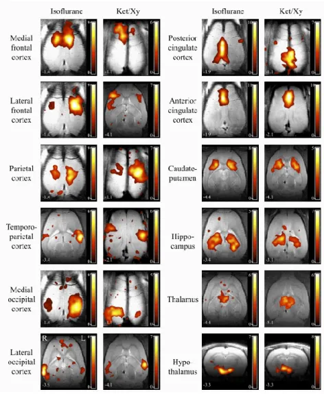
II.2.1.2. Anaesthetics: mechanisms of action ... 89
II.2.1.3. Impact of anaesthesia on global BOLD signal ... 91
II.2.1.4. Impact of anaesthetics on neuronal network organization ... 92
II.2.1.5. Anaesthetics used in rodents and primate for resting-state fMRI studies... 93
II.2.2. Introduction to the methodology: MRI sequences ... 95
II.2.3. Coregistration of EPI images ... 98
II.2.4. Signal pre-treatment for resting-state fMRI ... 100
II.2.5. Submitted article: Garin, C. M., Nadkarni, N. A., Landeau, B., Chételat, G., Picq, J-L, Bougacha, S., & Dhenain, M. (2019). Resting state cerebral networks in mouse lemur primates: from multilevel validation to comparison with humans. ... 103
II.3. Study 3: Resting-state fMRI and glutamate measures in the brain of a non-human primate: relationships and age-related alterations ... 153
II.3.1. Combination of fMRI and to other techniques ... 153
II.3.1.1. Electrophysiology and fMRI ... 154
II.3.1.2. Positron emission tomography and fMRI ... 155
II.3.1.3. NMR spectroscopy and fMRI ... 156
II.3.1.4. Other techniques evaluating neuronal activity characteristics ... 157
II.3.2. Article in preparation: Garin, C. M., Nadkarni, N. A., Pepin J., Bougacha, S., Flament, J. & Dhenain, M. (in preparation). Resting-state fMRI and glutamate measures in the brain of a non-human primate: relationships and age-related alterations. ... 159
III. Discussion ... 192
III.1. From anatomical to functional atlases in mouse lemurs ... 192
III.1.1. Comparison of anatomical to functional atlases ... 192
III.1.2. Graph theory features in mouse lemur brains ... 195
III.2. Methodological considerations concerning our studies ... 195
III.2.1. Implementation of Sammba-MRI ... 195
III.2.2. Anaesthesia and image acquisition protocols ... 196
III.2.3. fMRI image processing ... 197
III.3. Perspective of the studies ... 199
IV. Annexe ... 200
IV.1. Résumé ... 200
IV.2. Scientific production: ... 203
IV.2.1. Oral scientific communications: ... 203
IV.2.2. Invited talk: ... 203
7 IV.2.4. In preparation ... 205 IV.2.5. Other contributions ... 205 V. Bibliography... 248
8
Figures
Figure 1 | Mouse lemur. ... 14
Figure 2 | Aged related atrophy in the mouse lemur brain.. ... 15
Figure 3 | BOLD signal: magnetic susceptibility to vascular oxygenation. ... 19
Figure 4 | Blood vessel detection with a gradient echo sequence in the rat brain... 19
Figure 5| BOLD hemodynamic response function following a single brief stimulus. ... 20
Figure 6 | BOLD response to stimuli in the visual cortex. ... 21
Figure 7 | BOLD correlation in the motor cortex under activation and at rest... 22
Figure 8 | Human default mode network characterized by seed-based correlation analysis. ... 24
Figure 9 Group-ICA analysis at rest: Assumption of the number of components. ... 26
Figure 10 | Four modules detected in the human brain. ... 28
Figure 11 | Comparison of different networks based on their large scale topological properties. ... 30
Figure 12 | Major resting-state networks of the human brain. ... 32
Figure 13 | Default mode network discovered for the first time in the macaque brain. 35 Figure 14 | Eleven independent components extracted from fMRI images of the macaque brain. ... 36
Figure 15 | Synthesis of the macaque DMNs observed in rsfMRI literature. ... 37
Figure 16 | Four large scale networks extracted from the macaque brain using various seeds in the cingulate cortex. ... 39
Figure 17 | Reproducible cerebral networks in rats under two types of anaesthesia.. . 40
Figure 18 | Similar components are extracted in rats and mice.. ... 42
Figure 19 | Functional regions identified via ICA in the mouse brain using twenty components. ... 43
Figure 20 | DMN identified with ICA in the mouse brain using five components. ... 44
Figure 21 | The mouse lemur brain. ... 52
Figure 22 | Voxel movement parameters. ... 55
Figure 23 | Extracting the brain from anatomical images... 55
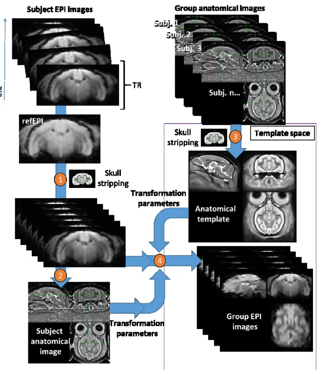
Figure 24 | Four major steps for the fMRI image coregistration to an anatomical template. ... 99
Figure 25 | Association between two rsfMRI networks and their EEG profiles. ... 155
Figure 26 | Brain regions identified as decreasing their activity during cognitive tasks. ... 156
Figure 27 | Mouse lemur 3D functional atlas based on dictionary learning ... 194
9
Table
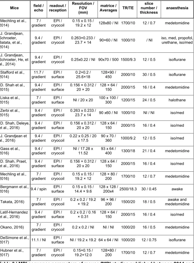
Table 1 | Anaesthetic effects on the functional connectivity in rodents. ... 94 Table 2 | Anaesthetic effects on the functional connectivity in primates. ... 95 Table 3 | MRI sequence parameters of mouse fMRI studies published between 2014 and 2017. ... 96 Table 4 | MRI sequence parameters of rat fMRI studies published between 2011 and 2017. ... 97
10
List of abbreviations
ALFF amplitude of low-frequency fluctuation
BOLD blood-oxygen level dependent
CSF cerebrospinal fluid
DMN default mode network
EEG electroencephalography
FC functional connectivity
fMRI functional magnetic resonance imaging
gluCEST exchange saturation transfer imaging of glutamate
ICA independent component analysis
MRI magnetic resonance imaging
NHP non-human primates
PET positron emission tomography
RS resting-state
rsfMRI resting-state functional magnetic resonance imaging
12
Summary and aim of the thesis
Animal models are routinely used to mimic diseases in order to explore the impact of pathological processes on brain networks or to measure the effect of a new therapy. The mouse lemur (Microcebus murinus) is a primate that has attracted attention within neuroscience research. This small animal is a model for studying cerebral aging and various diseases such as diabetes-related encephalopathy, Parkinson's disease, or Alzheimer's disease. It has a key position on the phylogenetic tree of primates and is used to investigate primate brain evolution. Its cerebral anatomy is still poorly described and its cerebral networks have never been investigated.
The first objective of this study was to develop new tools to develop a 3D digital atlas of the brain of this model and to use this atlas to automatically follow-up brain characteristics in cohorts of animals. A common question for the study of cohorts of animals by MRI is the ability to register large series of images including images recorded with different protocols. We developed a Python package called sammba-MRI to generate specific cerebral templates and to coregister various images to this template. This package offers an efficient integration of existing coregistration methods (ANTS, AFNI). This package was used to create a template of mouse lemur brains to create a digital atlas of the mouse lemur brain. This atlas and several other available mammalian atlases have permitted to compare the regional brain volumes amongst species. Measures from MRI atlases indicate that white matter to cerebral volume index increased from rodents to small primates to macaques, reaching their highest values in humans.
Studies of cerebral connectivity have contributed to many breakthroughs in the understanding of brain function in normal as well as in pathological conditions such as Alzheimer’s or Parkinson’s diseases. The second objective of this work was to characterize cerebral connectivity in mouse lemurs. This study was based on the evaluation of mouse lemur brains after resting-state blood-oxygen level dependent (BOLD) functional magnetic resonance imaging (fMRI). Patterns of low-frequency signal oscillations recorded with this technique are similar in brain structures functionally connected. Dedicated MR protocols were developed and sammba-mri was used to coregister fMRI images. Then, we created a methodology to extract and
13
characterize, for the first time, cerebral networks in the mouse lemur. We showed that their brain is organised into local functional regions integrated into large scale functional networks. They were classified as default-mode-like, control-executive-like, motor, visual, basal ganglia and thalamic networks and compared to large scale networks in humans. We highlighted common organisation rules but also discrepancies between these two species.
The biological parameters associated to the organization of brain region into networks are still poorly understood. In a last part of the study, we characterized the relationship between resting-state fMRI and glutamate levels assessed by Chemical Exchange Saturation Transfer imaging of glutamate (gluCEST). We highlighted a relationship between the amplitude of low-frequency fluctuations (ALFF), a measure of cerebral activity issued from rsfMRI as well as hubness and glutamate level, which suggests that glutamate has a critical role on organization and regulation of brain function. A relationship between hubness, local neuronal activity and an index of glutamate level in the brain is consistent with the well-established role of glutamate as an excitatory neurotransmitter. More precisely we found that glutamate is strongly associated to ALFF in the cortical and subcortical brain regions. In the cortex, glutamate is also associated to functional connectivity (hubness). We also highlighted age-related changes for these parameters. They concern alterations of ALFF in the default mode network and reduction of glutamate in the globus pallidus. We also highlighted an age-related reorganization of the cortical/subcortical relationships between ALFF and functional connectivity.
14
I. Introduction
I.1. Overview of the mouse lemur primate
The mouse lemur (Microcebus murinus; Figure 1) or gray mouse lemur is a prosimian non-human primate (NHP). It was first described in 1777 by the English illustrator John Frederick Miller. Phylogenetically the mouse lemur is classified in the Primate order, the Strepsirrhini sub-order, the infra order of the Lemuriforms and the family of the Cheirogaleidae. The Lemuriforms infra order is entirely endemic to Madagascar. The Cheirogaleidae are composed of 5 genera Microcebus, Mirza, Allocebus, Cheirogaleus, and Phaner weighing from 30g to 600g. They are all quadrupeds and mostly have an elongated body and short legs. They are nocturnal
species and sleep in small nests or holes in a tree (Mittermeier et al., 2008). Although the mouse lemur is probably the most abundant mammalian species native to Madagascar, its trade for commercial purposes has been prohibited since 1975 by the Convention on International Trade of Endangered Species (CITES).
Figure 1 | Mouse lemur.
Morphologically the mouse lemur is characterized by its small size, around 25 to 28 centimetres including a tail length of 13 to 14.5 centimetres. Its body mass varies during the seasons (summer ≈ 75 grams, winter ≈ 120 grams). Seasonal variations can be reproduced in captivity by changing the photoperiod: long days (light >12h/day) correspond to summer i.e. the dry season and a short day (light <12h/day) correspond to winter i.e. the rainy season. These physiological variations are also characterized by torpor, a lower temperature and a hypometabolism in winter which facilitates the accumulation of fat reserves (Kobbe et al., 2014). These physiological modifications are uncommon in a primate species. The mouse lemur’s diet in the wild is composed
15
of leaves, flowers, nectar, fruits and insects. In captivity it is composed of gingerbread, fruits (such as banana and apple), eggs and concentrated milk. Like many mammalian species, the mouse lemur has seasonal breeding (end of the dry season) with at most 3 estrus lasting 1 to 5 days for the females. The gestation latency (60 days) results in 1 to 4 progenies weighing around 5 grams. Young mouse lemurs reach maturity quickly (≈ 6 to 8 months).
The mouse lemur has a short lifespan in comparison to homologous primates, but has a remarkable longevity for a mammal of its size. The lifespan of the mouse lemur is around 4 years in the wild, due to high predation, but can reach 12 years in captivity (Perret, 1997). Interestingly, the mouse lemur is considered old at around 6 years and displays age-related alterations. As it ages, a decrease in its sensory function (hearing, olfaction, visual acuity) and motor activity are observed(Beltran et al., 2007) (Nemoz-Bertholet et Aujard, 2003)(Languille et al., 2012). MRI studies also described important
cerebral atrophies linked to an increase of the cerebro-spinal fluid (CSF) surrounding
the brain and within the ventricles (Dhenain et al., 2000)(Figure 2). This atrophy occurs in 60% of the aged lemurs (Kraska et al., 2011) with an important variability of atrophy patterns.
Figure 2 | Aged related atrophy in the mouse lemur brain. Anatomical MRI images of a non-atrophied (5.5 years, a) and atrophied (8.8 years, b) mouse lemur brain. The arrow shows CSF inclusion surrounding the cerebral cortex. Adapted from (Kraska et al., 2011).
Cognitive alterations related to the atrophy severity in the hippocampus and the entorhinal cortex are reported in the aged mouse lemur (Picq et al., 2012). Numerous studies have explored Alzheimer-like pathology (N. Bons et al., 2006; Kraska et al., 2011) while aging in the mouse lemur. The Alzheimer’s disease-like pathological
16
changes were mainly defined by the accumulation of amyloid plaques occurring in about 20% of the aged lemurs (Noëlle Bons et al., 1992) and some rare tauopathy (Giannakopoulos et al., 1997). More recently, mouse lemurs were used to artificially induce Parkinson's (Mestre-Frances et al., 2018) or Alzheimer's diseases (Gary et al., 2015). Mouse lemurs were also used to evaluate different therapies. Pifferi et al. found that an Omega-3 fatty acid supplementation (Fish oil) enhances the resting-state glucose consumption of the lemur’s brain (Pifferi et al., 2015). Another recent study found that caloric restriction increases lifespan of the lemurs but affects their brain integrity (Pifferi et al., 2018). Moreover, the key position of mouse lemurs on the phylogenetic trees of primates, makes this animal an important model to investigate primates’ brain evolution (Montgomery et al., 2010).
Despite its use to evaluate physio-pathological changes, several improvements remain to be performed to characterize this animal. First, its brain was characterized using 2D anatomical atlas (N. Bons et al., 1998) (Zilles et al., 1979) (Le Gros Clark, 1931). New digital atlases are required to improve the possible use of this animal. Cerebral function is also poorly assessed in mouse lemurs. Here, we developed dedicated tools to create a 3D digital atlas of its brain. We also developed new protocols to characterize cerebral connectivity in mouse lemurs. We finally characterized glutamate-based mechanisms associated to the organization of their brains in neuronal networks and reported age-related changes modulating their cerebral function. Further presentation of the rationale leading to each study is presented before the presentation of an article focusing on each study.
I.2. Magnetic resonance imaging: from anatomy to brain networks I.2.1. Magnetic resonance imaging: basics
Magnetic resonance imaging (MRI) is a non-invasive and non-ionizing technique that is used to create images of the body. It is routinely used in the clinic for diagnosis and in preclinical research to explore different tissue characteristics/contrasts. In addition to anatomy, MRI permits the detection of several physiological properties such as, spatial diffusion of water, metabolite concentration or blood flow and oxygenation. Nuclear magnetic resonance was discovered by Bloch and Purcell in 1946 (Bloch, 1946) (Purcell et al., 1946). The theory is that most atomic nuclei such as hydrogen or
17
phosphorus have a property called “spin” or spin angular momentum. Spin can be orientated when absorbing the energy produced by a magnetic field. Thus, applying a magnetic field (B0) upon nuclei polarize and align their spin parallel (low-energy state)
or perpendicular (high-energy state) to this field (Grover et al., 2015). However, not all nuclei are aligned to B0 and the proportion of the aligned nuclei results in a net
magnetization (M). The higher the magnetic field of the MRI, the higher the net magnetization. The energy state of a nucleus can be changed by applying a radiofrequency field (B1). These radiofrequencies are commonly applied in pulses
lasting microseconds that cause energy transition of the nucleus from low to high. The absorbed energy is subsequently emitted by the nucleus, generating an oscillating current within a reception coil and this process is called “free-induction decay” (FID). The resonance frequency needed to induce a transition of energy can be calculated by the equation of Larmor. The Larmor frequency (ω0) is dependent on a constant for
each nucleus (γN) and the strength of the magnetic field (B0).
ω0 = γN. B0
Thus, the frequency required to resonate a nucleus in a given magnetic field can be established for each magnetic field. The localization of MR signal is performed using gradient to create B0 field strength variations. The signal is encoded into two
dimensions (frequency and phase) to create a 2D image or slice using the Fourier transform equation. The combination of this principle with the slice selective excitation pulse allows the spatial localization of the signal within a three-dimensional (3D) space.
Differentiating two tissues with anatomical MRI is often based on their relaxation properties that modify the signal intensity. The hydrogen nucleus (single proton) is the most studied nucleus because of its abundance in fat and water. A difference in relaxation properties between two tissues, changes the rate at which each nucleus returns to its thermal equilibrium. This process is called T1 relaxation or longitudinal
relaxation and measures the time until the magnetization returns to its thermal equilibrium. The transverse relaxation (T2) is the disappearance of the transverse
magnetization. It is due to the energy exchange between spins, which induces a loss of phase coherence in the transverse plane and therefore a progressive disappearance of the transverse magnetization. The T2* is referred to as T2 but also considers local
18
parameters in a sequence such as the time between two excitatory radiofrequency pulses (repetition time) and time between the excitation pulse and the signal peak (echo time) “weights” the image toward a contrast T1 or T2. As an example, using T1
contrast, brain tissues can be separated based on their distinctive contrasts producing low signal intensity within the brain ventricles (dark), medium intensity within the gray matter, and high intensity within the white matter (bright). This T1/T2 difference is one of the mechanisms that provide contrast by MRI.
Practically, acquisition of MR images reposes on the use of dedicated acquisition sequences that are particular setting of pulse sequences and pulsed field gradients that allow to record spins in a particular state. The two basic sequences are spin-echo and gradient echo sequences. The spin echo-sequence is based on the application of a 90° pulse followed up by a 180° pulse, prior to acquisition of the signal from an echo. This sequence can be adjusted to give T1-weighted, proton density, and T2-weighted images. Gradient echo sequences were initially based on a single pulse varying from 5 to 90 degrees followed-up by an echo that is recorded. This sequence provides T1-weighted, proton density, and T2*-weighted images. Larger flip angles give more T1 weighting to the image and the smaller flip angles give more T2* weighting to the images. These basic sequences have been largely complexified to provide new contrasts and faster imaging schemes.
I.2.2. BOLD signal
Blood oxygenation level dependent (BOLD) imaging is the standard technique used to generate images in functional MRI (fMRI) studies. It relies on the measure of cerebral blood flow and oxyhemoglobin/deoxyhemoglobin state of haemoglobin that evolve when neurons from a brain region are activated (Boniface, 2002). The reason fMRI is able to detect this change is due to a fundamental difference in the paramagnetic properties of oxyhemoglobin and deoxyhemoglobin. Deoxygenated hemoglobin is paramagnetic whereas oxygenated hemoglobin is not leading to different signal in images (Figure 3). Heavily T2* weighted sequences are used to detect this change, which is in the order of 1-5% (Gore, 2003).
19 Figure 3 | BOLD signal: magnetic susceptibility to vascular oxygenation. The MRI signal within the deoxygenated tissue is lower because of the field inhomogeneity generated by the deoxyhemoglobin paramagnetic properties. The field inhomogeneity lead to a faster decay of the signal. From (Gore, 2003)
BOLD signal was discovered in 1990 by Ogawa et al. (Seiji Ogawa et al., 1990). They described tubular hypo-intensities in the rodent cortex that were visible with a T2*-weighted sequence but not with a T2-weighted (Figure 4)Erreur ! Source du renvoi introuvable.. They also highlighted for the first time, the paramagnetic effect of the deoxygenated blood on the MRI contrast (S. Ogawa et al., 1990).
Figure 4 | Blood vessel detection with a gradient echo sequence in the rat brain. Gradient echo epi (a) and spin echo epi (b) image acquired in an anoxic mouse brain. Tubular intensities corresponding to blood vessels can be detected with gradient echo epi sequence. From (Seiji Ogawa et al., 1990)
20
Following the initial work by Ogawa et al., several groups characterized the relationships between neuronal activation by a task and evolution of the BOLD signal. They showed that following a stimulus, the BOLD signal show a small initial dip, followed by a tall peak, and then a variable post-stimulus undershoot(Barth et Poser, 2011) (Figure 5).
Figure 5 | BOLD hemodynamic response function following a single brief stimulus. From (Barth et Poser, 2011).
The initial dip origin remains highly debated. It might reflect a quick extraction of the blood oxygen prior to any cerebral blood flow increase. The initial dip is found in many non-human species such as rats, cats and monkeys and is specific towards neuronal activity (K.-S. Hong et Zafar, 2018). The main response or peak is usually delayed by approximately 2 seconds. This interval could correspond to the time in which the blood travels from arteries to draining veins and capillaries (Logothetis, 2003). The bulk of the BOLD response is mediated by a variety of biological mechanisms contributing to the hemodynamic response such as: blood flow, blood volume, increases in deoxyhemoglobin concentration and oxygen metabolism. After the stimulus, a decrease of the BOLD signal is typically observed and called undershoot. The undershoot origin is also disputed and supposedly reflects an increase of the cerebral blood flow overcompensating for the oxygen increase (Logothetis, 2003).
Thus, the BOLD signal is assumed to indirectly measure the neuronal activity in a process called neurovascular coupling (Murakami et al., 2018).
21
I.2.3. From BOLD signal to evoked functional MRI
BOLD signal is largely used to characterize cerebral activity following activation with various stimuli (i.e. motor (Bandettini et al., 1994), speech (Hinke et al., 1993) or cognitive tasks (Buckner et al., 1996). The use of this technique to infer on brain function relies on block task paradigm. It corresponds to a series of trials (i.e resting and activity task) performed during a period of time. The signal acquired during these two blocks can be compared statistically. Blamire et al. was one of the first studies detecting a BOLD signal increase in the visual cortex in response to an external stimulus (flashing checkerboard) (Blamire et al., 1992) (Figure 6).
Figure 6 | BOLD response to stimuli in the visual cortex. BOLD signal total response from voxels extracted in the visual cortex. The BOLD signal peak exhibits a delay between the task (ON = 2 seconds) and its response. From (Blamire et al., 1992).
One of the major steps toward the wide use of BOLD fMRI was the development of fast imaging sequences permitting the acquisition of multiple images during a resolute period of time (Cohen et Weisskoff, 1991) in order to perform efficient blocked task paradigms.
I.2.4. From BOLD signal to resting-state functional MRI
Further analyses of BOLD-fMRI signal have also led to another major discovery, i.e. the existence of spontaneous and elaborated patterns of neuronal activity in the human brain at rest (B. Biswal et al., 1995). By exploring the correlated activity of the motor cortex for a finger-tapping experiment, Biswal et al. found during a baseline session that interhemispheric coordinated activity occurs even in the absence of stimuli (B.
22
Biswal et al., 1995)(Figure 7). Rapidly, this technique is coming to be used to describe a large set of brain areas connected by spontaneously coordinated activities at rest. These connected areas are defined as resting-state networks (Guye et al., 2008). The default-mode network, salience network, sensory motor network, visual networks are amongst the most widely described networks. We will focus on the description of cerebral networks characterized in humans (“I.4.1. Organization and function of cerebral networks in humans”) and in animals (“I.4.2. Organization and function of cerebral networks in non-human primates”). The analysis of resting-state networks is based on image processing algorithms that will be described in the following paragraph
Figure 7 | BOLD correlation in the motor cortex under activation and at rest. This figure displays on the left (a) the correlated voxel corresponding to the activation paradigm (finger tapping). Coordinated activity is observed in the right and the left hemisphere of the motor cortex. Similar coordinated activity was observed at rest (b) and in similar areas. From (B. Biswal et al., 1995).
I.3. Overview of the methods used to characterize cerebral networks by resting-state fMRI
I.3.1. Overview of image acquisition schemes for rsfMRI
fMRI technique is based on the images acquisition at low spatial resolution. Thanks to this low spatial resolution, it is possible to obtain an excellent temporal resolution which produces images of the whole brain every 1 to 5 seconds. The total acquisition time of an fMRI scan can last a few minutes (usually between 5 and 15 minutes) resulting in hundreds of images covering the entire brain (or one 4D image with three spatial dimensions and one temporal dimension). The different slices of a single brain
23
image are not acquired at the same time. An interleaved acquisition (1, 3, 5…) is commonly used to reduce the “slice cross-talk artefacts”. The intensity of the voxels of a 4D fMRI image varies by a low percentage over time. However, this small variation can be detected with the algorithms described in the following paragraphs.
I.3.2. From signal to functional connectivity analysis
Functional connectivity is the connectivity between brain regions that share functional properties. More specifically, it can be defined as the temporal correlation between spatially remote neurophysiological events, expressed as deviation from statistical independence across these events in distributed neuronal groups and areas (B. B. Biswal et al., 1997). Several algorithms have been implemented to analyze this connectivity. We will present the most widely used algorithms.
I.3.2.1. Seed-based correlation analysis
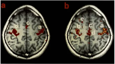
Seed-based correlation analysis is one of the most common methodologies for functional network characterization (Greicius et al., 2003) (Figure 8). This method was first adopted by Biswal et al. to explore Pearson's correlation coefficients between voxelwise signals and ROIs or “seeds” (B. Biswal et al., 1995). The seed is a small area, used to extract and average the BOLD signal. It can be defined by creating either a sphere corresponding to the coordinates of brain regions or by using regions predetermined by a brain atlas. The Pearson's correlation coefficients can be measured between the signal extracted within the seed and the voxelwise signals. The reconstruction of the Pearson's correlation coefficients corresponding to each voxel in the 3D space of the brain image highlights areas connected to the seed.
24 Figure 8 | Human default mode network characterized by seed-based correlation analysis.
Map of the resting-state default mode networks highlighted by the voxels connected to the posterior cingulate cortex (seed, blue arrow). Significant clusters are found in (A&C) inferior parietal cortex, (B) orbitofrontal cortex, ventral anterior cingulate cortex, (D&G) medial prefrontal cortex, (E) dorsolateral prefrontal cortex, (F) parahippocampal gyrus, (H) inferolateral temporal cortex. From (Greicius et al., 2003).
I.3.2.2. Analyses based on BOLD signal spatial decomposition
Network organization can also be explored by using spatial decomposition algorithms. Two main algorithms were developed in order to extract brain networks on raw images: (1) independent component analysis (ICA) and (2) dictionary learning. Both produce a set of activation 3D maps that permit the characterization of the cerebral networks. Although these algorithms are more complex than the seed based correlation analysis, the identification of co-activated areas remains based on the same basic principle.
(1) ICA was the first algorithm developed and adapted for fMRI images. This computational algorithm assumes that several areas of the brain can be separated into different spatially or temporally independent sources of signal called components. One of the assumptions of ICA is that the components display a non-Gaussian signal. The two broadest definitions of independence for ICA are the maximization of the non-Gaussianity and the minimization of mutual information.
25
(2) The dictionary learning method identifies a sparse representation (component) of an array that can form a linear combination. The array or 2D matrix is extracted using an fMRI image (column = brain voxels; rows = time points). One advantage to dictionary learning is that it allows repeated use of brain voxels, meaning that the same voxel could be included in different components. This property provides an improved flexibility of decomposition. Both methods have succeeded in separating functional regions from rsfMRI datasets. Their limitation is that the number of components has to be estimated prior to the analysis and this assumption greatly affects the ICA or dictionary learning results (Figure 9). Clear segmentation differences between two similar components could appear. For example, the components of Figure 9 (A; 24) and (B; 69) define the same network (executive) and are characterized by the anterior cingulate cortex. Their extraction using 27 (A) and 70 (B) components leads to the non-detection of several co-activated areas in (A; 24) compared to (B; 69). The other limitation specific to ICA, is that this algorithm struggles to reveal networks with partly neuro-anatomical overlaps (W. Zhang et al., 2019). This issue is a limitation for ICA since brain networks are not segregated in space but interact with each other. Indeed, the brain is a heterogeneous entity with intermixed neurons and various axonal projections within the same region.
26 Figure 9 | Group-ICA analysis at rest: Assumption of the number of components. Group-ICA in humans based on 27 components (A) where 16 were found non-artefactual and 70 components (B) where 12 were found non-artefactual. From (Tian et al., 2013).
27
I.3.2.3. Analyses based on graph analysis and hub identification
Graph theory is another technique to characterize local functional regions as well as large-scale networks. With graph theory, whole brain networks (graph) are defined as a set of nodes (basic elements of the system) and edges (allowing relationships between nodes). The correlations of the BOLD fMRI signal between the different nodes provides an index of functional connectivity (FC) (C. F. Beckmann et al., 2005; J. S. Damoiseaux et al., 2006) and are represented by the edges of the network.
In graph theory, large scale networks can be defined as modules or communities, which are groups of nodes densely connected by edges and sparsely connected with nodes from other modules. One of the most common methods to divide a network into communities is called modularity maximization. Modularity is a metric comparing the number of edges of a community and evaluating their differences with equivalent random communities (M. E. Newman, 2006). High modularity means dense connection within a module and sparse connection between nodes of different modules. Modularity maximization assigns a different community to each node and evaluates the gain of modularity if node A is removed from its community and placed in community X(D. B. Vincent et al., 2008). The community detection is useful for the automatic partition of a network into distinct communities that are relevant to the neurological organization of the brain (Figure10). However, modularity maximization
suffers from methodological limitations such as the existence of partitions that are equally optimal. Also, this algorithm cannot classify nodes in different modules (overlapping nodes) which is a problem for biological relevance (see chapter: I.3.2.2. Analyses based on BOLD signal spatial decomposition).
28
Figure 10 | Four modules detected in the human brain.
The detected modules were based on a network in which each voxel represents a node. These four networks are consistent with the current knowledge of the human brain organization explored with other techniques. From (Moussa et al., 2012).
Whole brain networks can also be characterized using various descriptors of
topological properties. For example, "hubness" describes the degree of node
centrality or its influence in the network which is supposedly related to its importance for brain function. Eigenvector centrality was used as a hubness descriptor in our studies. However, a wide variety of descriptors exist, representing different hubness features in a given graph. Standard hubness metrics are:
- Eigenvector centrality that detects nodes highly connected to other highly connected nodes (Lohmann et al., 2010). Eigenvector centralitymeasures the centrality of a node according to the number of links it has with other nodes in the network. Eigenvector centrality also considers the connection quality of a node, the number of links it has, and so on for the whole network. Eigenvector centrality calculates the extended connections of a node, so it favors nodes that influence the entire network and is not limited to direct connections.
29
- Degree centrality simply represents the number of edges of a node (or the mean of their value on a weighted graph). Degree centrality find highly connected nodes that are likely to hold most of the information which can connect quickly with the larger network.
- Closeness centrality identifies the shortest path between two nodes and calculates the sum of its edges. It is estimated for a given node, by averaging the sum of the edges of the shortest path between the node and all other nodes in the graph (van den Heuvel et al., 2010).
- Betweenness centrality detects the amount of times a node appears on the shortest path along other nodes. It considers the influence of a node as its "bridges" property. To do this, it detects the shortest paths of the entire network and counts number of times a given node lie into it (van den Heuvel et al., 2010). This metric is probably the most commonly used to characterize hubness. - Current flow betweenness centrality is a betweenness centrality measure
that also considers the influence from all the paths across nodes. This algorithm provides more weight to the shortest path but also considers the other connections. Interestingly, the information is considered to spread as an electrical current (M. E. J. Newman, 2005).
To our knowledge, there is no consensus for the best hub metric to characterize brain networks.
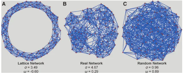
Small-worldness is another index of topological properties of the network. It
defines large scale specialization and global information transfer efficacy. It can be characterized using two small-world coefficients (σ and ω) (NetworkX (Hagberg et al., 2008))(Figure 11).
σ is defined as σ = 𝐶/Crand
𝐿/Lrand (Watts et Strogatz, 1998)
ω is defined as ω = 𝐿
Lrand− 𝐶
Crand (Telesford et al., 2011).
With C and L being, respectively, the average clustering coefficient (a measure of network segregation) and the average shortest path length (a measure of integration) of the network. Crand and Lrand are their equivalent derived random networks.
Small-30
world networks have σ values superior to 1 and ω values close to 0 (Telesford et al., 2011). The small-world coefficients are disrupted in several neuropathologies such as Alzheimer’s disease (X. Zhao et al., 2012) or schizophrenia (Anderson et Cohen, 2013).
Figure 11 | Comparison of different networks based on their large scale topological properties.
Equivalent lattice (A), real (B), random (C) networks. The networks that are considered as small-world are the lattice (σ= 3.49) and the real world (σ= 4.67). From (Telesford et al., 2011).
31
I.4. Functional connectivity in mammalian species
I.4.1. Organization and function of cerebral networks in humans
Resting-state networks have been largely described in humans (Figure 12) (B. Biswal et al., 1995; B. B. Biswal et al., 2010; Fox et Raichle, 2007). Their study has contributed to many breakthroughs in understanding the relationship between human cognition and brain architecture (Mather et al., 2013).
The most studied resting-state network is the DMN (Figure 12 ; Figure 26 ; Figure 8). It was first described by Raichle et al. (Raichle et al., 2001) using positron emission tomography (PET). This network is particularly engaged during rest and is suspended/deactivativated during stimulated brain activity (Hampson et al., 2006; Tambini et al., 2010). The main regions implicated in the DMN are posterior cingulate cortex, medial prefrontal cortex, and medial, lateral, and inferior parietal cortices. The DMN is possibly involved in memory consolidation (Huo et al., 2018) or other cognitive functions such as mindfulness (Doll et al., 2015), self-referential and introspective state (Greicius et al., 2003). The DMN is often divided into two major networks (anterior and posterior DMN). The anterior DMN is more active during self-directed thoughts and the posterior DMN during passive rest (C. G. Davey et Harrison, 2018). Also, Davey et al. investigated the DMN during self-related processes and found that the posterior cingulate cortex is mainly implicated in the coordination of the mental representations. The medial prefrontal cortex is a regulator or ‘gateway’ function of self-representations (C. G. Davey et al., 2016). Furthermore, the DMN may prove to be implicated in and/or be an indicator of healthy and non-healthy brain aging including several pathological processes such as Alzheimer’s or Parkinson’s diseases (Buckner et al., 2005; Gao et Wu, 2016). Moreover, the pattern of deposition of one the major lesions in Alzheimer’s disease (amyloid plaques), co-localizes with the DMN(Buckner et al., 2005).
32 Figure 12 | Major resting-state networks of the human brain. Adapted from (Raichle, 2011)
The executive-control network (Figure 12) embeds regions from the superior and middle prefrontal cortex, anterior cingulate cortex, paracingulate gyri, ventrolateral prefrontal cortex and subcortical regions of the thalamus (Christian F. Beckmann et al., 2005; Mazoyer et al., 2001). The executive network is especially active during tasks involving target-directed, intellectual activities and participation in cognitive control. Anti-correlated activity is reported in this network at rest(Seeley et al., 2007a). Patients with attention-deficit/hyperactivity display a higher functional connectivity within the anterior cingulate cortex related to a decrease in their symptoms (Francx et al., 2015). The attention network (Figure 12) is commonly divided into two separate fronto-parietal networks (dorsal and ventral) that both involve different areas of the frontal cortex (Vossel et al., 2014). The dorsal attention network embeds the intraparietal sulcus, as well as the frontal eye field. This network is implicated in attention processes such as the selection of stimuli (spatial cueing of color, shape, motion direction). Also,
33
this network is involved in the control of appropriate response, potentially mediated by a selection (top-down) of the cognitive stimuli and actions(Hopfinger et al., 2000). The ventral attention network involves the ventral frontal cortex and the temporo-parietal junction(Vossel et al., 2014). This network seems dedicated to the spatial attention of new stimuli (visual, sound and tactile) (Vossel et al., 2006). Therefore, the main function evoked for this network is the reorientation of the attention to relevant stimuli (Stevens et al., 2005).
The salience network (Figure 12) includes regions in the dorso-medial prefrontal cortex, anterior cingulate cortex, insula, and temporo-parietal junction. This network is associated with mindfulness and the regulation of the dynamic changes with other networks implicated in mindfulness (DMN or the control-executive)(Doll et al., 2015). The main function of the salience network is probably to regulate the switch between networks. It participates in answering to salient events by facilitating the access to working memory, attention or motor systems(Menon et Uddin, 2010). Other roles of this network are related to moral reasoning (Chiong et al., 2013), resistance to temptation(Steimke et al., 2017) and more global emotional and empathic functions (Seeley et al., 2007b). Dysfunctions of the network are associated with neuropsychiatric disorders such as autism, schizophrenia and frontotemporal dementia(Uddin, 2014).
The visual network (Figure 12) was divided into two main large- scale networks(J. S. Damoiseaux et al., 2006): (1) medial visual cortical areas composed of the primary visual area located in the calcarine sulcus, medial extrastriate nucleus and lingual gyrus (Christian F. Beckmann et al., 2005) as well as co-activated areas in thelateral geniculate nucleus precuneus regions. The thalamus is proposed as a “relay station” from the visual input to the primary visual cortex (Christian F. Beckmann et al., 2005). (2) lateral visual cortical areas including mainly non-primary visual areas such as the occipital pole and the occipito-temporal cortex as well as superior parietal regions. This set of regions is assumed to have a role in visuo-spatial attention or visual attention (Christian F. Beckmann et al., 2005). Some studies have demonstrated that lesions within the parietal regions can disturb spatial attention(Nachev et Husain, 2006).
The sensory-motor network (Figure 12; Figure 7) was the first rsfMRI found by Biswal et al. (B. Biswal et al., 1995) using seed-based analysis. This network is mainly
34
composed of regions from the pre and postcentral gyri (Brodmann areas 1, 2 and 3) and the supplementary motor area. The sensory-motor network display high interhemispheric correlations(Bharat B. Biswal, 2012). The primary sensory cortex and the primary motor cortex can be subdivided into areas responsible for the processing of sensory and motor information dedicated to specific areas of the body such as the nose, eyes, toes, etc.(Grodd et al., 2001).
The auditory network (Figure 12) involves the primary and secondary auditory cortices and is dedicated to the process of auditory stimuli. An asymmetry of this network is highly debated(Andoh et al., 2015).
The basal ganglia network is mainly composed of the caudate nucleus, putamen, pallidum, substantia nigra and subthalamic nucleus (Afifi, 2003). This network is associated with a variety of functions such as motivational, emotional, motor and cognitive processes (Bednark et al., 2015). This network is highly damaged in Parkinson's disease and Huntington's disease(Wen et al., 2012) and the functional connectivity matrix of this network was used to classify Parkinson's disease patients versus healthy controls with 81% accuracy(Rolinski et al., 2015).
This list of networks is not exclusive and other major networks have been described in humans. We cannot describe all these networks here.
35
I.4.2. Organization and function of cerebral networks in non-human primates
Cerebral networks have been described in non-human primates as in humans. The first characterization of cerebral networks in anesthetized non-human primates at rest found four large scale networks (J. L. Vincent et al., 2007) classified as the DMN, oculomotor, somatomotor and visual. They were anatomically close to those previously described in humans. This major discovery highlighted that the brain functional organization transcends the consciousness and reflects an evolutionarily conserved property of the primate brain.
Figure 13 | Default mode network discovered for the first time in the macaque brain.
Significant voxels correlated to the posterior cingulate cortex (seed-based analysis) in anesthetized macaque using BOLD fMRI. Adapted from (J. L. Vincent et al., 2007).
These results were quickly confirmed by Rilling et al. using [18
F]-fluorodeoxyglucose PET on awake chimpanzees at rest (Rilling et al., 2007) and later with [15O]H2O PET in macaques (Kojima et al., 2009). In 2009, the posterior cingulate
cortex activity measured by electrophysiology was found to be suppressed during task performance and returned to a higher resting baseline at rest in macaques (Hayden et al., 2009). Hutchison et al. was the first to analyze fMRI images with ICA (20 components) on the macaque (Macaca fascicularis) cortex and found 11 relevant components ((R. M. Hutchison et al., 2011); Figure 14)
36 Figure 14 | Eleven independent components extracted from fMRI images of the macaque brain.
The ICA was performed using 20 components, 11 were selected as relevant and named as follows: A: precentral–temporal; B: fronto-parietal; C: posterior-parietal; D: occipito-temporal; E: frontal; F: superior-temporal; G: cingulo-insular; H: paracentral; I: parieto-occipital; J: postcentral; K: hippocampal. From (R. M. Hutchison et al., 2011)
37
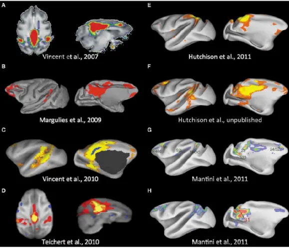
A meta-analysis of macaque fMRI images has allowed a comparison of the reduction of activity during goal-directed behavior within the DMN rather than the functional connectivity analysis at rest or under anaesthesia (D. Mantini et al., 2011). This publication was followed by a meta-analysis synthesizing all the DMN organization descriptions of macaques published before 2012 (R. M. Hutchison et Everling, 2012). This article found a diversity of anatomical clusters included in this network (Figure 15).
Figure 15 | Synthesis of the macaque DMNs observed in rsfMRI literature.
(A) (J. L. Vincent et al., 2007), (B) (Margulies et al., 2009), (C) (J. L. Vincent et al., 2010), (D) (Teichert et al., 2010), (E, F) (R. M. Hutchison et al., 2011), (G, H) (D. Mantini et al., 2011). From (R. M. Hutchison et Everling, 2012).
38
Different articles reported common features as well as discrepancies between the macaque DMN. (J. L. Vincent et al., 2007) and (Margulies et al., 2009) found similar correlated activity (seed-based analysis) in the lateral temporoparietal cortex, the posterior parahippocampal cortex, the dorsal medial prefrontal cortex and the anterior cingulate cortex; (D. Mantini et al., 2011) and (J. L. Vincent et al., 2010) found similar correlated activity in the dorsal medial prefrontal cortex and in the inferior parietal lobule. However, the lateral temporoparietal cortex and the posterior parahippocampal cortex were absent; (Teichert et al., 2010) and (R. M. Hutchison et al., 2011) did not find medial and dorsal frontal and hippocampal regions. Differences features of the macaque DMN were explained by the limitations of seed-based analyses and by the use of different seeds in various studies. Indeed, different seeds locations or sizes could potentially impact the reproducibility of the features (R. M. Hutchison et Everling, 2012). The use of ICA was proposed as a solution to provide more reproducible results.
In chimpanzees, DMN regions similar to those reported in humans were proposed (medial prefrontal cortex, posterior cingulate cortex and precuneus) (Barks et al., 2015). The DMN is also found in awake marmosets, recruiting the retrosplenial and posterior cingulate cortices, medial parietal area, premotor and posterior parietal areas and areas surrounding the intraparietal sulcus (Belcher et al., 2013).
Other large scale networks similar to those detected in humans are observed in the non-human primates at rest. For example, using different seeds in the cingulate cortex Hutchison et al. identified four large scale networks (somatomotor, executive, attention-orienting and limbic) ((R. M. Hutchison et al., 2012); Figure 16).
39 Figure 16 | Four large scale networks extracted from the macaque brain using various seeds in the cingulate cortex. From (R. M. Hutchison et al., 2012)
The salience network has also been described in the macaque brain but its identification is not justified on a behavioral/functional basis (Touroutoglou et al., 2016).
In the awake marmoset, the diversity and the number of networks extracted with ICA (eleven) was exceptionally high (higher-order visual, basal ganglia, primary visual, dorsal (medial) somatomotor, higher-order visual, higher-order midline visual, default mode, salience, orbitofrontal, cerebellar, ventral (lateral) somatomotor, frontal pole). The frontal-parietal network was recently described in the marmoset brain and is characterized as a major network (high hubness score) (Ghahremani et al., 2016).
As evoked for the DMN and other networks, difficulties occurred in describing the spatial limits between distinct networks and in identifying their functions. These difficulties generated different conclusions concerning the identifications of several large scale networks. A standardized methodology will be necessary in order to obtain reproducible results across laboratories.
40
I.4.3. Organization and function of cerebral networks in rats
As in non-human primates, rat cerebral networks were first discovered under anaesthesia. One of the first studies to observe correlated areas with fMRI signals in rats was performed with a 9.4T MRI. It found two networks corresponding to the sensorimotor and visual networks (Pawela et al., 2008). One year after this discovery, Zhao discovered a caudate/putamen network in rats (F. Zhao et al., 2008). Later, a large list of reproducible networks that were extracted with ICA was proposed by Hutchiston et al. under two types of anaesthesia ((R. M. Hutchison et al., 2010); Figure
17).
Figure 17 | Reproducible cerebral networks in rats under two types of anaesthesia. Rat networks were extracted from rsfMRI images using an ICA with 40 components. From (R. M. Hutchison et al., 2010).
41
Modularity algorithms have also been used to describe the rat cerebral network organization. Using partial correlations, with 36 anatomical regions D'Souza et al. found two pure cortical (frontal, somato-motor) and four mixed large scale networks (hippocampal and perihippocampal cortices, basal ganglia, thalamic nuclei and pons, Q=0.39) (D'Souza et al., 2014).
A similar organization was found in awake rats (N. Zhang et al., 2010) (Becerra et al., 2011) including a network analogous to the human DMN. The rat DMN was described in several publications(Upadhyay et al., 2011)(Lu et al., 2012). According to Lu et al., the co-activated clusters of the rat DMN are the orbital cortex, prelimbic cortex, cingulate cortex, auditory/temporal association cortex, posterior parietal cortex, retrosplenial cortex (corresponding to the posterior cingulate cortex in humans) and the hippocampus(Lu et al., 2012). As in non-human primates, rsfMRI networks have been compared to humans. Sierakowiak et al. (Sierakowiak et al., 2015) found four remarkable similarities between rat rsfMRI networks and human networks (DMN, motor, dorsal basal ganglia and ventral basal ganglia). These results are particularly interesting for the development of translational experiments to validate animal models of brain disorders. However, the DMN regions extracted from this study were different when compared to the study of Lu et al. This difficulty to identify a reproducible pattern of network organization is probably due to the multiple levels of systems and subsystems that may support distinct functions, as suggested by Hsu et al. and Smith et al. (Hsu et al., 2016) (Smith et al., 2009).
The advantage of using rats is that numerous pathological models of brain disorders have been developed. As a consequence, alterations of the rat functional connectivity or of network organization are studied in various neuropathological models such as Alzheimer’s disease (Sanganahalli et al., 2013), Parkinson's disease (Westphal et al., 2017), stress (Henckens et al., 2015) and aging (Ash et al., 2016).
42
I.4.4. Organization and function of cerebral networks in mice
One of the first publications describing and comparing rat and mouse rsfMRI network organization highlighted the difficulties of cross-species comparison. The extracted maps remain highly dependent on the ICA components number that can skew the results (Jonckers et al., 2011). However, comparing two species with the same number of components remains potentially more accurate than using seed based-analysis. As for primates ((R. M. Hutchison et al., 2012); Figure 16) the localization of a seed within the same region could totally change the type of network detected. As a consequence, in order to accurately compare two equivalent networks across species, the anatomical correspondence of the seeds has to be known prior to the analysis. To our knowledge, these criteria are rarely met. The methodological strength of the study by Jonckers et al. was the use of two ICA component numbers which allowed them to evaluate the stability of the extracted maps across the two species and to identify that the components of the mouse brain are more unilateral than rats (Jonckers et al., 2011)(Figure 18).
Figure 18 | Similar components are extracted in rats and mice. ICA applied to rat and mouse rsfMRI with 15 and 40 components. The components in the mouse brain seem to be more unilateral than in rats. From (Jonckers et al., 2011).
These two levels of ICA (low and high number of components) have also been studied in several studies in humans (Smith et al., 2009), and mice (F. Sforazzini et al., 2014). Sforazzini et al. explored the functional brain of mice by varying the number at a high level (20 components; Figure 19) and low level (5 components; Figure 20) (F.
43
Sforazzini et al., 2014). The ICA using 20 components resulted in maps encompassing several established neuro-anatomical systems of the mouse brain (Figure 19).
Figure 19 | Functional regions identified via ICA in the mouse brain using twenty components.
The ICA was performed on BOLD images. IC1: pre-frontal cortex, IC2, cingulate/retrosplenial cortex, IC3 and IC4, anterior and posterior parietal (somatosensory) cortex; IC5, anterior motor cortex, IC6, posterior motor cortex, IC7, thalamus, IC8, caudate putamen, IC9, dorsal hippocampus, IC10, cerebellum and brain stem. Abbreviations: aMc, anterior motor cortex; aPc, anterior parietal cortex; Cb, cerebellum; Cg, cingulate cortex; CPu, caudate-putamen; Hc, dorsal hippocampus; PFc, prefrontal cortex; pMc, posteriormotor cortex; pPc, posterior parietal cortex; Rs, retrosplenial cortex; Th, thalamus. From (F. Sforazzini et al., 2014).
44
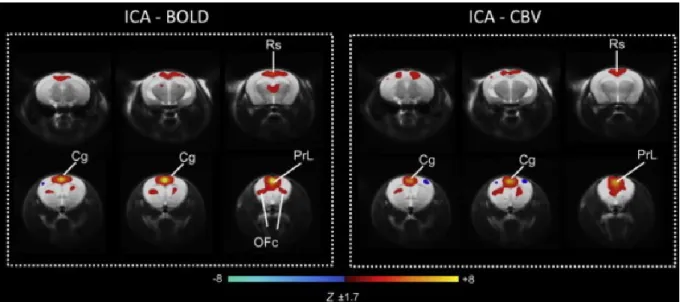
Interestingly, the low level ICA applied to BOLD images (Figure 20; left) highlighted a putative DMN in mice that was very similar to the DMN-like network observed in the same study with a seed-based approach and CBV weighted images (Figure 20; right)
Figure 20 | DMN identified with ICA in the mouse brain using five components.
The ICA was performed on BOLD and CBV weighted images. Abbreviations: Acb, nucleus accumbens; Cg, cingulate cortex; OFc, orbitofrontal cortex; Pc, parietal cortex; Prl, prelimbic cortex; Rs, retrosplenial cortex. From (F. Sforazzini et al., 2014).
This study also observed anti-correlations between the mouse DMN and the neighboring fronto-parietal regions which is consistent with literature based on human studies. However, as in rat and non-human primates, the regions thought to be involved in the DMN are highly debated. Sforazzini et al. found that the DMN includes the nucleus accumbens, cingulate cortex, orbitofrontal cortex, parietal cortex, prelimbic cortex and the retrosplenial cortex (F. Sforazzini et al., 2014). Stafford et al. found a DMN encompassing the parietal cortex, the lateral/medial orbital cortex and the cingulate area (Stafford et al., 2014). For Zerbi et al. this network covers the caudomedial entothinal cortex, cingulate cortex area, caudate putamen, medial entorhinal cortex, medial orbital cortex, parasubiculum, prelimbic cortex, retrosplenial
dysgranular and granular cortex and the thalamus (Zerbi et al., 2015).
As previously discussed for other species, these studies have clearly highlighed the difficulty in identifying reproducible cerebral networks. Morever, this difficulty is accentuated by the extremly small size of the mouse brain (around 400 mm3). Other