HAL Id: hal-01148846
https://hal.inria.fr/hal-01148846
Submitted on 13 May 2015
HAL is a multi-disciplinary open access
archive for the deposit and dissemination of
sci-entific research documents, whether they are
pub-lished or not. The documents may come from
teaching and research institutions in France or
abroad, or from public or private research centers.
L’archive ouverte pluridisciplinaire HAL, est
destinée au dépôt et à la diffusion de documents
scientifiques de niveau recherche, publiés ou non,
émanant des établissements d’enseignement et de
recherche français ou étrangers, des laboratoires
publics ou privés.
typed object calculus
Daniel J. Dougherty, Pierre Lescanne, Luigi Liquori
To cite this version:
Daniel J. Dougherty, Pierre Lescanne, Luigi Liquori. Addressed term rewriting systems: application to
a typed object calculus. Mathematical Structures in Computer Science, Cambridge University Press
(CUP), 2006, 16 (issue 4), pp.667-709. �10.1017/S096012950600541X�. �hal-01148846�
Addressed Term Rewriting Systems:
Application to a Typed Object Calculus
Daniel J. Dougherty1 and Pierre Lescanne2 and Luigi Liquori3
1 Department of Computer Science, Worcester Polytechnic Institute Worcester, MA 01609 USA.
2 Laboratoire de l’Informatique du Parallélisme, École Normale Supérieure de Lyon 46, Allée d’Italie, 69364 Lyon 07, FRANCE.
3 INRIA Sophia Antipolis FR-06902 FRANCE.
Received 14 October 2005; Revised 26 March 2006
We present a formalism called Addressed Term Rewriting Systems, which can be used to model implementations of theorem proving, symbolic computation, and programming languages, especially aspects of sharing, recursive computations and cyclic data structures. Addressed Term Rewriting Systems are therefore well suited for describing object-based languages, and as an example we present a language called λOba, incorporating both functional and object-based features. As a case study in how reasoning about languages is supported in the ATRS formalism a type system for λOba is defined and a type soundness result is proved.
1. Introduction
1.1. Addressed Calculi and Semantics of Sharing
Efficient implementations of functional programming languages, computer algebra sys-tems, theorem provers, and similar systems require some sharing mechanism to avoid multiple computations of a single argument. A natural way to model this sharing in a symbolic calculus is to pass from a tree representation of terms to directed graphs. Such term-graphs can be considered as a representation of program-expressions intermediate between abstract syntax trees and concrete representations in memory, and term-graph rewriting provides a formal operational semantics of functional programming sensitive to sharing. There is a wealth of research on the theory and applications of term-graphs; see for example (Barendregt, et al. 1987, Sleep, et al. 1993, Plump 1999, Blom 2001) for general treatments, and (Wadsworth 1971, Turner 1979, Ariola & Klop 1994, Ariola & Klop 1996, Ariola, et al. 1995, Ariola & Arvind 1995) for applications to λ-calculus and implementations.
This paper bridges two approaches to the implementation of functionally or declar-ative programming language, namely graph rewriting and term rewriting. The former provides an abstract approach for an efficient implementation whereas the latter is closer
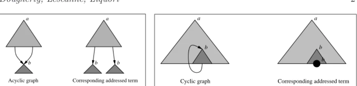
Corresponding addressed term Acyclic graph a b b a b b a a
Cyclic graph Corresponding addressed term
b b
Figure 1. Sharing and Cycles Using Addresses
to ordinary mathematical notation and so stays closer to our intuition. The theory here applies to languages such as pure ML (Milner, et al. 1997, Leroy, et al. 2004), Haskell (Peyton Jones, et al. 2003), Clean (Plasmeijer & van Eekelen 2001), logic lan-guages like Prolog (Kowalski 1979) or rule-based lanlan-guages like Maude (Clavel, et al. 2003), Elan (Borovansky, et al. 1998) or Cafe-OBJ (Diaconescu & Futatsugi 1998).
In this paper we annotate terms, as trees, with global addresses in the spirit of (Felleisen & Friedman 1989, Rose 1996, Benaissa, et al. 1996). The approach to labeled term rewrit-ing systems of Ohlebusch (Ohlebusch 2001) is similar to our formalism (in the acyclic case); Lévy (Lévy 1980) and Maranget (Maranget 1992) previously introduced local
ad-dresses. From the point of view of the operational semantics, global addresses describe
better what is going on in a computer or an abstract machine.
Labeling intermediate terms with addresses is a novel technique for the analysis of the implementation of functional languages. A standard treatment would consist of translat-ing a big-step rewrittranslat-ing semantics into an abstract machine (Diehl, et al. 2000). In our formalism addresses are part of the evaluation-terms and they are de facto decorated with locations. As a consequence the small-step semantics given by rewriting and the abstract machines are strictly coupled: the thesis is that machine implementation can be accurately modeled by term rewriting.
The formalisms of term-graph rewriting and addressed-term rewriting share much sim-ilarity but we feel that the addressed-term setting has several advantages. Our intention is to define a calculus that is as close to actual implementations as possible with the view of terms as tree-like structure, and the addresses in our terms really do correspond to memory references. To the extent that we are trying to build a bridge between theory and implementation we prefer this directness to the implicit coding inherent in a term-graph treatment.
With explicit global addresses we can keep track of the sharing that can be used in the implementation of a calculus. Sub-terms that share a common address represent the same sub-graphs, as suggested in Figure 1 (left), where a and b denote addresses. In (Dougherty, et al. 2002), addressed terms were studied in the context of addressed
term rewriting, as an extension of classical first-order term rewriting. In addressed term
rewriting we rewrite simultaneously all sub-terms sharing a same address, mimicking what would happen in an implementation.
We also enrich the sharing with a special back-pointer to handle cyclic graphs (Rose 1996). Cycles are used in the functional language setting to represent infinite data-structures and (in some implementations) to represent recursive code; they are also
interesting in the context of imperative object-oriented languages where loops in the
store may be created by imperative updates through the use of self (or this). The idea
of the representation of cycles via addressed terms is rather natural: a cyclic path in a finite graph is fully determined by a prefix path ended by a “jump” to some node of the prefix path (represented with a back-pointer), as suggested in Figure 1 (right).
The inclusion of explicit indirection nodes is a crucial innovation here. Indirection nodes allow us to give a more realistic treatment of the so-called collapsing rules of term-graph rewriting (rules that rewrite a term to one of its proper sub-terms). More detailed discussion will be found in Section 2.
1.2. Suitability of Addressed TRS for describing an Object-based Formalism
Recent years have seen a great deal of research aimed at providing a rigorous foundation for object-oriented programming languages. In many cases, this work has taken the form of “object-calculi” (Fisher, et al. 1994, Abadi & Cardelli 1996, Gordon & Hankin 2000, Igarashi, et al. 2001).
Such calculi can be understood in two ways. On the one hand, the formal system is a specification of the semantics of the language, and can be used as a formalism for classifying language design choices, to provide a setting for investigating type systems, or to support a denotational semantics. Alternatively, we may treat an object-calculus as an intermediate language into which user code (in a high-level object-oriented language) may be translated, and from which an implementation (in machine language) may be derived.
Several treatments of functional operational semantics exist in the literature (Landin 1964, Augustson 1984, Kahn 1987, Milner, et al. 1990). Addressed Term Rewriting Systems (originally motivated by implementations of lazy functional programming lan-guages (Peyton-Jones 1987, Plasmeijer & van Eekelen 1993)) are the foundation of the
λOba formalism (Lang, et al. 1999) for modeling object-oriented languages. The results in (Lang et al. 1999) showed how to model λOba using Addressed Term Rewriting Sys-tems, but with no formal presentation of those systems. Here we expose the graph-based machinery underneath the rewriting semantics of λOba. To our knowledge, term-graph rewriting has been little explored in the context of the analysis of object-based program-ming.
The novelty of λOba is that it provides a homogeneous approach to both functional and object-oriented aspects of programming languages, in the sense the two semantics are treated in the same way using addressed terms, with only a minimal sacrifice in the permitted algebraic structures. Indeed, the addressed terms used were originally introduced to describe sharing behavior for functional programming languages (Rose 1996, Benaissa et al. 1996).
A useful way to understand the λOba formalism is by analogy with graph-reduction as an implementation-calculus for functional programming. Comparing λOba with the implementation techniques of functional programming (FP) and object oriented pro-gramming (OOP) gives the following correspondence. The λOba “modules” L, C, and F are defined in section 3.
Paradigm λOba fragment Powered by
Pure FP λOba (L) ATRS
Pure FP+OOP λOba (L+C+F) ATRS
1.3. Outline of the Paper
The paper is organized as follows: Section 2 details the formalism of addressed term rewriting systems and establishes a general relation between addressed term rewriting systems and first-order term rewriting systems. Section 3 puts addressed term rewriting systems to work by presenting the three modules of rewriting rules that form the core of
λOba. For pedagogical convenience we proceed in two steps: first we present the calculus
λObσ, intermediate between the calculus λOb of Fisher, Honsell and Mitchell (Fisher et al. 1994) and our full calculus λOba, then we scale up to λObaitself. Section 4 presents a running object-based example in the λOba formalism. Section 5 addresses the rela-tionship between λOb and λOba. Section 6 proposes a type system for λOba. Section 7 concludes. In appendix A we give a connection between a kind of ATRS’s and TRS’s.
This paper is an extended version of (Dougherty, et al. 2005) and originated in research presented in (Lang et al. 1999).
2. Addressed Term Rewriting Systems
In this section we introduce addressed term rewriting systems or ATRS. Classical term rewriting (Dershowitz & Jouannaud 1990, Klop 1990, Baader & Nipkow 1998) cannot easily express issues of sharing and mutation. Calculi that give an account of memory management often introduce some ad-hoc data-structure to model the memory, called
heap, or store, together with access and update operations. However, the use of these
structures necessitates restricting the calculus to a particular strategy. The aim of ad-dressed term rewriting (and that of term-graph rewriting) is to provide a mathematical model of computation that reflects memory usage and is robust enough to be independent of the rewriting strategy.
Sharing of computation. Consider the reduction square(x) → times(x, x). In order to
share subterms, addresses are inserted in terms making them addressed terms. For in-stance if we are to compute square(square(2)), we attach addresses a, b, c to the individual subterms. This yields squarea(squareb(2c)) which can then be reduced as follows:
squarea(squareb(2c)) Ã timesa(squareb(2c), squareb(2c)) timesa(timesb(2c, 2c), timesb(2c, 2c)) Ã timesa(4b, 4b) Ã 16a,
where “Ô designates a one step reduction with sharing. The key point of a shared computation is that all terms that share a common address are reduced simultaneously.
Sharing of Object Structures. It is important not only to share computations, but also to
share structures. Indeed, objects are typically structures that receive multiple pointers. As an example, if we “zoom” on Figure 7, we can observe that the objects p and q share
a common structure addressed by b. This can be very easily formalized in the formalism, since addresses are first-class citizens. See Section 4.
Cycles. Cycles are essential in functional programming when one deals with infinite
data-structures, as in lazy functional programming languages. Cycles are also used to save space in the code of recursive functions. Moreover in the context of object programming languages, cycles can be used to express loops which can be introduced in memory via lazy evaluation of recursive code.
2.1. Addressed Terms
Addressed terms are first order terms whose occurrences of operator symbols are
deco-rated with addresses. They satisfy well-formedness constraints ensuring that every ad-dressed term represents a connected piece of a store. Moreover, the label of each node sets the number of its successors. Addresses intuitively denote node locations in memory. Iden-tical subtrees occurring at different paths can thus have the same address corresponding to the fact that the two occurrences are shared.
The definition is in two stages: the first stage defines the basic inductive term structure, called preterms, while the second stage just restricts preterms to well-formed preterms, or addressed terms.
Definition 2.1 (Preterms).
1 Let Σ be a term signature, and • a special symbol of arity zero (a constant). Let A be an enumerable set of addresses denoted by a, b, c, . . ., and X an enumerable set of
variables, denoted by X, Y, Z, . . . An addressed preterm t over Σ is either a variable X,
or •a where a is an address, or an expression of the form Fa(t
1, . . . , tn) where F ∈ Σ (the label) has arity n ≥ 0, a is an address, and each ti is an addressed preterm (inductively).
2 The location of an addressed preterm t, denoted by loc(t), is defined by
loc¡Fa(t
1, . . . , tn) ¢4
= loc(•a)4
=a,
3 The sets of variables and addresses occurring within a preterm t are denoted by var (t) and addr (t), respectively, and defined in the obvious way.
Example 2.1. The following are preterms
—timesa(timesb(2c, 2c), timesb(2d, 2c))
—timesa(timesb(2c, 2c), timesb(2c, 2c))
—timesa(timesb(•c, •c), timesb(•c, •c))
The first is “ill-formed” in the sense that the two subterms labeled with b are not the same; the latter two do not suffer from this anomaly, and are examples of what we call an admissible term: see Definition 2.4. For the first preterm above we have
—loc(timesb(2d, 2c))) = loc(timesb(2c, 2c))) = b,
—var (timesa(timesb(x, x), timesb(x, x))) = {x},
Addresses signify locations used to store a concrete term in memory; an open preterm t (a preterm with variables) is a notation to capture the family of concrete instantiations of t, and so the variables in t itself are never realized themselves. For this reason we do not assign addresses to variables in a term; they are meant to be replaced by addressed terms lying at any address.
The definition of a preterm makes use of a special symbol • called a back-pointer and used to denote cycles (Rose 1996). A back-pointer •a in an addressed term must be such that a is an address occurring on the path from the root of the addressed term to the back-pointer node. It simply indicates at which address one has to branch (or point back) to go on along an infinite path.
Example 2.2. The infinite list made of 0’s will be represented as consa(0b, •a) and we can look for the 5thelement, by applying the function nth, as follows: nthc(5b, consa(0b, •a)). An essential operation that we must have on addressed (pre)terms is the unfolding that allows seeing, on demand, what is beyond a back-pointer. Unfolding can therefore be seen as a lazy operator that traverses one step deeper in a cyclic graph. It is accompanied with its dual, called folding, that allows giving a minimal representation of cycles. Note however that folding and unfolding operations have no operational meaning in an actual implementation (hence no operational cost) but they are essential in order to represent correctly transformations between addressed terms.
Definition 2.2 (Folding and Unfolding).
Folding.Let t be a preterm, and a be an address. We define fold(a)(t) as the folding of
preterms located at a in t as follows: fold(a)(X)4 =X fold(a)(•b)4 =•b (a ≡ b allowed here) fold(a)¡Fa(t1, . . . , tn) ¢4 =•a fold(a)¡Fb(t1, . . . , tn) ¢4 =Fb¡fold(a)(t1), . . . , fold(a)(tn) ¢ if a 6≡ b
Unfolding.Let s and t be preterms, such that loc(s) ≡ a (therefore defined), and a does not occur in t except as the address of •a. We define unfold(s)(t) as the unfolding of
•a by s in t as follows: unfold(s)(X) 4 =X unfold(s)(•b)4 = ( s if a ≡ b •b otherwise unfold(s)¡Fb(t1, . . . , tm) ¢4 =Fb¡t01, . . . , t0m ¢ where s0 4 =fold(b)(s) t0 1 4 =unfold(s0)(t 1) . . . t0 m 4 =unfold(s0)(t m) Given an address a, the intended meaning of folding is to replace all the subterm at
address a by •a, when unfolding does somewhat the opposite as it replaces •a by the term it corresponds to (i.e. at the same address) above it.
Example 2.3. fold(a)(nthc(5b, consa(0b, •a))) = nthc(5b, •a).
unfold(consa(0b, •a))(nthc(5b, consa(0b, •a))) = nthc(5b, consa(0b, consa(0b, •a))) We now proceed with the formal definition of addressed terms also called admissible preterms, or simply terms, for short, when there is no ambiguity. As already mentioned, addressed terms are preterms that denote term-graphs. From the point of view of ad-dresses, terms are preterms where at each address one finds basically the same term, i.e. the same term modulo an appropriate treatment of • or back pointers.
The notion of in-term helps to define addressed terms. The definition of addressed terms takes two steps: the first step is the definition of dangling terms, that are the sub-terms, in the usual sense, of actual addressed terms. Simultaneously, we define the notion of a dangling term, say s, at a given address, say a, in a dangling term, say t. When the dangling term t (i.e. the “out”-term) is known, we just call s an in-term. For a dangling term t, its in-terms are denoted by the function t @ _, read “t at address _”, which returns a minimal and consistent representation of terms at each address, using the unfolding.
Therefore, there are two notions to be distinguished: on the one hand the usual well-founded notion of “sub-term”, and on the other hand the (no longer well-well-founded) notion of “term in another term”, or “in-term”. In other words, although it is not the case that a term is a proper sub-term of itself, it may be the case that a term is a proper in-term of itself or that a term is an in-term of one of its in-terms, due to cycles. The functions
ti@ _ are also used during the construction to check that all parts of the same term are consistent, mainly that all in-terms that share a same address are all the same dangling terms.
Dangling terms may have back-pointers that do not point anywhere because there is no node with the same address “above” in the term. The latter are called dangling
back-pointers. For instance, timesa(•c, •c) has a dangling back-pointer, while consa(0b, •a) has none. The second step of the definition restricts the addressed terms to the dangling terms that do not have dangling back-pointers. The following defines dangling terms and the function t @ _ from addr(t) to dangling in-terms. Intuitively, t @ a returns the in-term of t at address a.
Definition 2.3 (Dangling Addressed Terms).
We define the set DT (Σ) of dangling addressed terms inductively and simultaneously define the function t @ _:
Variables. — Each variable X is in DT (Σ) — X @ _ is nowhere defined. Back-pointers. — •a ∈ DT (Σ) — •a@ a ≡ •a
Expressions. — t ≡ Fa(t
1, . . . , tn) ∈ DT (Σ) provided that
– F ∈ Σ of arity n,
– t1∈ DT (Σ), . . . , tn∈ DT (Σ) satisfy: b ∈ addr (ti) ∩ addr (tj) ⇒ ti@ b ≡ tj@ b, and
– a is an address satisfying a ∈ addr (ti) ⇒ ti@ a ≡ •a
— t @ a ≡ t; and if b ∈ addr(ti), b 6= a, t @ b ≡ unfold(t)(ti@ b).
Example 2.4. Let t = consa(0c, consb(1d, •a)). Then t@b = consb(1d, consa(0c, consb(1d, •a))). We say that consb(1d, •a) is a dangling term.
Admissible addressed terms are those where all •a do point back to something in t such that a complete (possibly infinite) unfolding of the term exists. The only way we can observe this with the t @ _ function is through checking that no •a can “escape” because this cannot happen when it points back to something.
Definition 2.4 (Addressed Term).
A dangling addressed term t is admissible if a ∈ addr (t) ⇒ t @ a 6≡ •a. An admissible dangling addressed term will be simply denoted an addressed term.
Example 2.5.
—The following are admissible terms:
– timesa(timesb(2c, 2c), timesb(2c, 2c)),
– nthc(5b, consa(0b, •a)),
– consa(0c, consb(1d, •a)).
It is easy to see that an in-term of an admissible term is admissible. 2.2. Addressed Term Rewriting
The reduction of an addressed term must return an addressed term (not just a preterm). In other words, the computation model (here addressed term rewriting) must take into account the sharing information given by the addresses, and must be defined as the
smallest rewriting relation preserving admissibility between addressed terms. Hence, a
computation has to take place simultaneously at several places in the addressed term, namely at the places located at the same address. This simultaneous update of terms corresponds to the update of a location in the memory in a real implementation.
In an ATRS, a rewriting rule is a pair of open addressed terms (i.e., containing vari-ables) at the same location. The way addressed term rewriting proceeds on an addressed term t is not so different from the way usual term rewriting does; conceptually there are four steps.
1 Find a redex in t, i.e. an in-term matching the left-hand side of a rule. Intuitively, an
addressed term matching is the same as a classical term matching, except there is a new kind of variables, called addresses, which can only be substituted by addresses.
2 Create fresh addresses, i.e. addresses not used in the current addressed term t, which
will correspond to the locations occurring in the right-hand side, but not in the left-hand side (i.e. the new locations).
3 Substitute the variables and addresses of the right-hand side of the rule by their new
values, as assigned by the matching of the left-hand side or created as fresh addresses. Let us call this new addressed term u.
4 For all a that occur both in t and u, the result of the rewriting step, say t0, will have
t0@ a ≡ u @ a, otherwise t0 will be equal to t.
We give the formal definition of matching and replacement, and then we define rewrit-ing precisely. The reader may find it useful to look ahead to section 2.3 where we provide examples of rewriting with ATRSs: this will help motivate the following technical defini-tions.
Definition 2.5 (Substitution, Matching, Unification).
1 Mappings from addresses to addresses are called address substitutions. Mappings from variables to addressed terms are called variable substitutions. A pair of an address substitution α and a variable substitution σ is called a substitution, and it is denoted by hα; σi.
2 Let hα; σi be a substitution and p a term such that addr (p) ⊆ dom(α) and var (p) ⊆
dom(σ). The application of hα; σi to p, denoted by hα; σi(p), is defined inductively
as follows: hα; σi(•a)4 =•α(a) hα; σi(X)4 =σ(X) hα; σi¡Fa(p 1, . . . , pm) ¢4 =Fα(a)(q 1, . . . , qm) and qi =4 fold(α(a)) ¡ hα; σi(pi) ¢
3 We say that a term t matches a term p if there exists a substitution hα; σi such that
hα; σi(p) ≡ t.
4 We say that two terms t and u unify if there exists a substitution hα; σi and an addressed term v such that v ≡ hα; σi(t) ≡ hα; σi(u).
We now define replacement. The replacement function operates on terms. Given a term, it changes some of its in-terms at given locations by other terms with the same address. Unlike classical term rewriting (see for instance (Dershowitz & Jouannaud 1990) pp. 252) the places where replacement is performed are simply given by addresses instead of paths in the term.
Definition 2.6 (Replacement).
is defined as follows: repl(u)(X)4 =X repl(u)(•a) 4 = ( u @ a if a ∈ addr(u) •a otherwise, repl(u)¡Fa(t 1, . . . , tm) ¢ 4 = ( u @ a if a ∈ addr (u) Fa¡repl(u)(t 1), . . . , repl(u)(tm) ¢ otherwise
The replacement of addressed term is the generalization of the usual notion of replace-ment for terms that takes account of addresses in two respects: terms at same address must be replaced simultaneously bullets must be unfolded appropriately to avoid dangling pointers.
An easy induction on the structure of dangling terms shows show Proposition 2.1 (Replacement Admissibility).
If t and u are addressed terms, then repl(u)(t) is an addressed term. We now define the notions of redex and rewriting.
Definition 2.7 (Addressed Rewriting Rule).
An addressed rewriting rule over Σ is a pair of addressed terms (l, r) over Σ, written
l à r, such that loc(l) ≡ loc(r) and var (r) ⊆ var (l). Moreover, if there are addresses a, b
in addr (l) ∩ addr (r) such that l @ a and l @ b are unifiable, then r @ a and r @ b must be unifiable with the same unifier.
The square redex, given at the beginning of this section, is an example of addressed rewriting rule. This example is somewhat simple, since rules may in general contain addresses, but Figure 6 contains plenty of examples of rules with addresses.
The condition var (r) ⊆ var (l) ensures that there is no creation of variables. The condition loc(l) ≡ loc(r) says that l and r have the same top address, therefore l and r are not variables.
Remark 2.1 (The right-hand side restriction). In the definition of rewriting rule we forbid the right-hand side to be a variable. It may appear that this limits th expres-sive power of ATRS’s. On the contrary this is an interesting feature of ATRS’s which highlights our attention to implementation concerns. Suppose for example that we were to have a rule Fa(x) → x, to be applied in an in-term Fa(tb) of a term. (Remember that variables have no addresses. ) Then Fa(tb) would be rewritten to tb. Do we intend that
tb is also at address a? If yes, this means we have to have a means to redirect all pointers to a toward b. Surely such acrobatics should not be part of a term-rewriting system – nor an implementation of rewriting! So we forbid such situations. We can still encode the rule capturing the equation F (x) = x, by using indirection nodes (see the paragraph on evaluation contexts in Section 3.2). In the case of the above rule Fa(x) → x, the trick would be to introduce a unary operator d_ea (the indirection) and replace the rule by Fa(x) → dxea
introduced to remove the indirection, for instance a rule Gb(dxea
) → Gb(x), which also fulfills the restriction.
Definition 2.8 (Redex).
A term t is a redex for a rule l à r, if t matches l. A term t has a redex, if there exists an address a ∈ addr (t) such that t @ a is a redex.
In the square example at the beginning of this section, both squarea(squareb(2c)) and squareb(2c) are redexes. Note that, in general, we do not impose restrictions as linearity in addresses (i.e. the same address may occur twice), or acyclicity of l and r. Besides redirecting pointers, ATRS create new nodes. Fresh renaming insures that these new node addresses are not already used.
Definition 2.9 (Fresh Renaming).
1 We denote by dom(ϕ) and rng(ϕ) the usual domain and range of a function ϕ.
2 A renaming is an injective address substitution.
3 Let t be a term having a redex for the addressed rewriting rule l à r. A renaming
αfresh is fresh for l à r with respect to t if dom(αfresh) = addr (r) \ addr (l) i.e. the
renaming renames each newly introduced address to avoid capture, and rng(αfresh) ∩
addr (t) = ∅, i.e. the chosen addresses are not present in t.
Proposition 2.2 (Substitution Admissibility).
Given an admissible term t that has a redex for the addressed rewriting rule l à r. Then
1 A fresh renaming αfresh exists for l à r with respect to t.
2 hα ∪ αfresh; σi(r) is admissible.
Proof. The admissibility of t and l ensures that the substitution hα; σi satisfies some
well-formedness property, in particular the set rng(σ) is a set of mutually admissible terms in the sense that the parts they share together are consistent (or in other words, the preterm obtained by giving these terms a common root, with a fresh address, is an addressed term).
The use of αfresh both ensures that all addresses of r are in the domain of the
substi-tution, and that their images by α will not clash with existing addresses.
The definition of substitution takes care in maintaining admissibility for such substi-tutions, in particular the management of back-pointers. These properties are sufficient to ensure the admissibility of hα ∪ αfresh; σi(r).
At this point, we have given all the definitions needed to specify rewriting. Definition 2.10 (Rewriting).
Let t be a term that we want to reduce at address a by rule l à r. Proceed as follows:
1 Ensure t @ a is a redex. Let hα; σi(l) 4
=t @ a.
2 Compute αfresh, a fresh renaming for l à r with respect to t.
3 Compute u ≡ hα ∪ αfresh; σi(r).
4 The result s of rewriting t by rule l à r at address a is repl(u)(t). We write the reduction t à s, defining “Ô as the relation of all such rewritings.
Theorem 2.1 (Closure under Rewriting).
Let R be an addressed term rewriting system and t be an addressed term. If t à u in R then u is also an addressed term.
Proof. The proof essentially walks through the steps of Definition 2.10, showing that
each step preserves admissibility.
Let R be an addressed term rewriting system and t be an addressed term rewritten by the rule l à r. All of t, l, and r, are admissible. For the rewrite to be defined, we furthermore know that t has a redex
t0 4
=t @ a ≡ hα; σi(l)
The term t0 is admissible and by Proposition 2.2, we can find a renaming α
fresh that is
fresh for l à r with respect to t0 and we know that u ≡ hα ∪ α
fresh; σi(r) is admissible.
Proposition 2.1 finally ensures that repl(u)(t) is admissible.
Actually ATRS generalize TRS and we show in appendix A that acyclic ATRS which do not mutate terms, i.e., which do not replace a subterm by another subterm in place actually simulate TRS’s.
2.3. Rewriting examples
Example 2.6. As an easy application of the definition of rewriting we can revisit our
square example, and see that timesa(squareb(2c), squareb(2c)) rewrites to timesa(timesb(2c, 2c), timesb(2c, 2c)). Example 2.7 (Cycles). Consider the term t = Hc(Fb(Ga(•b)), Ga(Fb(•a))), and l →
r = Ga(x) → Fa(x). We want to reduce t at address a. We first compute the matching
hα; σi = h{a 7→ a}; {x 7→ Fb(Ga(•b))}i. Since r does not contain fresh variables, then
σfresh= ∅. s = hα; σi(Fa(x)) = Fa(Fb(•a)). The result of rewriting is:
repl({a 7→ Fa(Fb(•a)), b 7→ Fb(Fa(•b))})(t) = Hc(Fb(Fa(•b)), Fa(Fb(•a))) The corresponding transformation on graphs is shown in Figure 2.
c c b b a a F G H H F F
Figure 2. Graph Rewrite equivalent to Addressed Term Rewrite of Example 2.7.
Example 2.8. Consider the term t = Ga(Hb(•a)), and the rule
We want to reduce t at address b. Note that there is a redex at address b even though it does not appear syntactically. Indeed, t @ b = Hb(Ga(•b)), and
match(Ha(Gb(x)))(Hb(Ga(•b))) = h{a 7→ b, b 7→ a}; {x 7→ Hb(Ga(•b))}i. We denote this matching by hα; σi. Note that σfresh = ∅ and s = hα; σi(Ha(x)) =
Hb(hα; {x 7→ •b}i(x)) = Hb(•b). The result of rewriting t is
repl({b 7→ Hb(•b)})(t) = G(Hb(•b))
Example 2.9 (Mutation). The following shows how side effects are performed, using the well-known example of setcar.
Consider the symbols nil of arity 0, and cons of arity 2, the constructors of lists. car, of arity 1 is the operator which returns the first element of a list, and setcar, of arity 2, the operator which affects a new value to the first element of the list, performing a side effect. We also have an infinite number of symbols denoted by 1, 2, . . . , n, . . ., and the operation plus of arity 2. At last, we have the special symbol d e of arity 1 denoting an indirection node. The rules for the definition of car and setcar are the following:
setcara(consb(y, z), x) → dconsb(x, z)ea (Set-Car) setcara(dzeb, x) → setcara(z, x) (Elim-Ind) cara(consb(nc, z)) → dncea (Car-n)
We omit a definition of plus here. Consider the term
t = pluse(carc(setcara(consb(1f, nilh), 2g)), card(consb(1f, nilh)))
in which the list consb(1f, nilh) appears twice, which means that it is shared. Starting by applying the rule for setcar, the reduction proceeds as follows:
t → pluse(carc(dconsb(2g, nilh)ea), card(consb(2g, nilh))) (Set-Car)
→ pluse(carc(consb(2g, nilh)), card(consb(2g, nilh))) (Elim-Ind)
→ pluse(2c, card(consb(2g, nilh))) (Car)
→ pluse(2c, 2d) (Car)
→ 4e (Plus)
On the other hand, starting by applying the rule for car, the computation proceeds as follows:
t → pluse(carc(setcara(consb(1f, nilh), 2g)), 1d) (Car)
→ pluse(carc(dconsb(2g, nilh)ea), 1d) (Set-Car)
→ pluse(carc(consb(2g, nilh)), 1d) (Elim-Ind)
→ pluse(2c, 1d) (Car)
→ 3e (Plus)
able to determine easily whether a system has side effects or not. For instance, a side effect appears clearly in the rule (Set-Car), since the term consb(y, z) becomes consb(x, z) whereas the rewriting takes place at address a in a term of shape setcara(¤, ¤). Rules which do not host such transformations have no side effect.
3. Modeling an Object-based Formalism via ATRS: λOba
The purpose of this section is to describe the top level rules of the λOba, a formalism strongly based on acyclic ATRS introduced in the previous section.
The formalism is described by a set of rules arranged in modules. The three modules are called respectively L, C, and F, and they will be introduced in Subsection 3.3.
Lis the functional module, and is essentially the calculus λσa
wof (Benaissa et al. 1996). This module alone defines the core of a purely functional programming language based on λ-calculus and weak reduction.
Cis the common object module, and contains all the rules common to all instances of object calculi defined from λOba. It contains rules for instantiation of objects and invocation of methods.
Fis the module of functional update, containing the rules needed to implement object update.
The set of rules L + C + F is the instance of λOba for functional object calculi. We do this in two steps:
1 first we present the functional calculus λObσ, intermediate between the calculus λOb of Fisher, Honsell and Mitchell (Fisher et al. 1994) and our λOba,
2 then we scale up over the full λOba.
By a slight abuse of terminology we may say that λOba is a conservative extension of
λObσ, in the sense that for computations in λOba and computations in λObσ return the same normal form (Theorems 5.1 and 5.2). Since a λOba-term yields a λObσ-term by erasing addresses and indirections, one corollary of this conservativeness is
address-irrelevance, i.e. the observation that the program layout in memory cannot affect the
eventual result of the computation. This is an example of how an informal reasoning about implementations can be translated in λOba and formally justified.
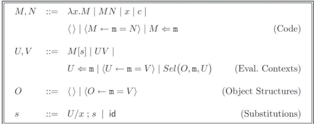
3.1. Syntax and operational semantics of λObσ
λObσis a language without addresses (see the syntax in Figure 3). The rules of λObσare presented in Figure 4. As noted earlier, terms of this calculus are terms of λObawithout addresses and without indirection nodes. The rules of λObσ are properly contained in those of modules L + C + F of λOba. One can also say that λObσis the lambda calculus
of objects proposed by Fisher, Honsell and Mitchell in (Fisher et al. 1994) enriched with
explicit substitutions. The first category of expressions is the code of programs. Terms that define the code have no addresses, because code contains no environment and is not subject to any change during the computation (remember that addresses are meant to tell the computing engine which parts of the computation structure can or have to
M, N ::= λx.M | M N | x | c |
h i | hM ← m = N i | M ⇐ m (Code)
U, V ::= M [s] | U V |
U ⇐ m | hU ← m = V i | Sel¡O, m, U¢ (Eval. Contexts)
O ::= h i | hO ← m = V i (Object Structures)
s ::= U/x ; s | id (Substitutions)
Figure 3. The Syntax of λObσ
Basics for Substitutions
(M N )[s] Ã (M [s] N [s]) (App) ¡ (λx.M )[s] U¢ Ã M [U/x ; s] (Bw) x[U/y ; s] Ã x[s] x 6≡ y (RVar) x[U/x ; s] Ã U (FVar) hM ← m = N i[s] Ã hM [s] ← m = N [s]i (P) Method Invocation (M ⇐ m)[s] Ã (M [s] ⇐ m) (SP) (O ⇐ m) Ã Sel(O, m, O) (SA) Sel(hO ← m = U i, m, V ) Ã (U V ) (SU)
Sel(hO ← n = U i, m, V ) Ã Sel(O, m, V ) m 6≡ n (NE)
Figure 4. The Rules of λObσ
change simultaneously). The second and third categories define dynamic entities, or inner structures: the evaluation contexts, and the internal structure of objects (or simply object
structures). The last category defines substitutions also called environments, i.e., lists of
terms bound to variables, that are to be distributed and augmented over the code.
Notation. The “ ; ” operator acts as a “cons” constructor for lists, with the environment
for lists we adopt the following aliases:
M [ ]a 4
= M [id]a
M [U1/x1; . . . ; Un/xn]a =4 M [U1/x1; . . . ; Un/xn; id]a
The code category is essentially the Lambda Calculus of Objects of (Fisher et al. 1994), and its operational semantics is the one presented in (Gianantonio, et al. 1998) and briefly recalled below:
(Gianantonio et al. 1998) Operational Semantics.
(λx.M ) N Ã M {N/x} (Beta)
M ⇐ m à Sel(M, m, M ) (Select)
Sel(hM ← m = N i, m, P ) Ã N P (Success)
Sel(hM ← n = N i, m, P ) Ã Sel(M, m, P ) m 6= n (Next) The main difference between λObσ and λOb (Fisher et al. 1994) lies in the use of a single operator ← for building an object from an existing prototype. If the object M contains m, then ← denotes an object override, otherwise ← denotes an object extension. The principal operation on objects is method invocation, whose reduction is defined by the (Select) rule. Sending a message m to an object M containing a method m reduces to
Sel(M, m, M ). The arguments of Sel in Sel(M, m, P ) have the following intuitive meaning
(in reverse order)
—P is the receiver (or recipient) of the message;
—m is the message we want to send to the receiver of the message;
—M is (or reduces to) a proper sub-object of the receiver of the message.
We note that the (Beta) rule above is given using the meta substitution (denoted by
{N/x}), as opposed to the explicit substitution used in λOba. Finally, the semantics presented in (Gianantonio et al. 1998) is not restricted to weak reduction (“no reduction under lambdas”) as is that in λOba.
By looking at the last two rewrite rules, one may note that the Sel function “scans” the recipient of the message until it finds the definition of the method we want to use. When it finds the body of the method, it applies this body to the recipient of the message. Notice that Sel somewhat destroys the object. In order to keep track of the objects on which the method when found has to be applied, a third parameter is added to Sel. 3.2. Syntax of λOba
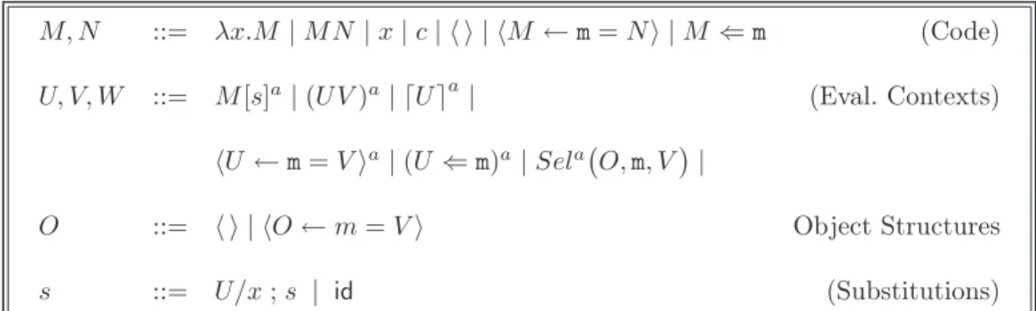
The syntax of λOba is summarized in Figure 5. As for λObσ terms that define the code have no addresses (the same for substitutions). In contrast, terms in evaluation contexts have explicit addresses.
“Fresh” addresses are often provided to evaluation contexts, when distributing the environment (a fresh address is an address unused in a global term). Intuitively, the address of an evaluation context is the address where the result of the computation will be
M, N ::= λx.M | M N | x | c | h i | hM ← m = N i | M ⇐ m (Code) U, V, W ::= M [s]a| (U V )a| dU ea | (Eval. Contexts) hU ← m = V ia| (U ⇐ m)a| Sela¡O, m, V¢| O ::= h i | hO ← m = V i Object Structures s ::= U/x ; s | id (Substitutions)
Figure 5. The Syntax of λOba
The Module L (M N )[s]a à (M [s]bN [s]c)a (App) ¡ (λx.M )[s]bU¢a à M [U/x ; s]a (Bw) x[U/x ; s]a à dU ea (FVar) x[U/y ; s]a à x[s]a x 6≡ y (RVar) (dU ebV )a à (U V )a (AppRed) The Module C (M ⇐ m)[s]a à (M [s]b ⇐ m)a (SP)
(U ⇐ m)a à Sela(U, m, U ) (SA)
(dU eb⇐ m)a à (U ⇐ m)a (SRed)
Sela(hU ← m = V ib, m, W ) Ã (V W )a (SU)
Sela(hU ← n = V ib, m, W ) Ã Sela(U, m, W ) m 6≡ n (NE)
Sela(dU eb, m, V ) Ã Sela(U, m, V ) (SelRed)
The Module F
hM ← m = N i[s]a à hM [s]b ← m = N [s]cia (FP)
hdU eb← m = V ia à hU ← m = V ia (FRed)
Figure 6. The Modules L and C and F
stored. A closure M [s]ais analogous to a closure in a λ-calculus, but it is given an address, and the terms in s are also addressed terms. The evaluation context dOea represents an object whose internal object-structure is O and whose object-identity is d ea. In other words, the address a plays the role of an entry point of the object-structure O. (O ←- m)a is the evaluation context associated to a method-lookup i.e., the scanning of the
object-structure to find the method m. ←- is an auxiliary operator, reminiscent to the selection operator Sel of λOb+, invoked when one sends a message to an object. We recall that the term •a is a back pointer. From object point of view they allow to create “loops in the store”. Only •acan occur inside a term having the same address a, therefore generalizing our informal notion of admissible term and simultaneous rewriting.
The Code Category. Code terms, written M and N , provide the following constructs:
—Pure λ-terms, constructed from abstractions, applications, variables, and constants. This allows the definition of higher-order functions.
—Objects, constructed from the empty object h i and a functional update operator
h_ ← _i. In a functional setting, this operator can be understood as extension as
well as override operator, since an override is handled as a particular case of extension.
—Method invocation (_ ⇐ _).
Evaluation Contexts. These terms, written U and V , model states of abstract machines.
Evaluation contexts contain an abstraction of the temporary structure needed to com-pute the result of an operation. They are given addresses as they denote dynamically instantiated data structures; they always denote a term closed under the distribution of an environment. There are the following evaluation contexts:
—Closures, of the form M [s]a, are pairs of a code and an environment. Roughly speak-ing, s is a list of bindings for the free variables in the code M .
—The terms (U V )a, (U ⇐ m)a, and hU ← m = V ia, are the evaluation contexts associ-ated with the corresponding code constructors. Direct sub-terms of these evaluation contexts are themselves evaluation contexts instead of code.
—The term Sela(U, m, V ) is the evaluation context associated to a method-lookup, i.e., the scanning of the context U to find the method m, and apply it to the context V . It is an auxiliary operator invoked when one sends a message to an object.
—The term dU ea denotes an indirection from the address a to the root of the addressed term U . The operator d_ea has no denotational meaning. It is introduced to make the right-hand side stay at the same address as the left-hand side. Indeed in some cases this has to be enforced. e.g. rule (FVAR). This gives account of phenomena well-known by implementers. Rules like (AppRed), (SRed) and (FRed) remove those indirections.
Remark 3.1 (ATRS-based preterms of λOba).
The concrete syntax of λOba of Figure 5 can be viewed as syntactic sugar over the definition of ATRS preterm in two ways:
1 Symbols in the signature may also be infix (like e.g., (_ ⇐ _)), bracketing (like
e.g., d_e), mixfix (like _[_]), or even “invisible” (as is traditional for application,
represented by juxtaposition). In these cases, we have chosen to write the address outside brackets and parentheses. For example we write (U V )ainstead of applya(X, Y ) and M [s]a instead of closurea(X, Y ) (substituting U for X, etc.).
It is clear that not all preterms denote term-graphs, since this may lead to inconsistency in the sharing. For instance, the preterm¡(h i[ ]b ⇐ m)ah i[ ]a¢c is inconsistent, because location a is both labeled by h i[ ] and¡_ ⇐ _¢. The preterm¡(dh i[ ]aeb
⇐ m)cdh i[ ]eeb¢d is inconsistent as well, because the node at location b has its successor at both locations a and e, which is impossible for a term-graph. On the contrary, the preterm¡(dh i[ ]aeb
⇐
m)cdh i[ ]aeb¢d
denotes a legal term-graph with four nodes, respectively, at addresses a, b,
c, and d†. Moreover, the nodes at addresses a and b, corresponding respectively to h i[ ] and h i[ ]a, are shared in the corresponding graph since they have several occurrences in the term. These are the distinction captured by the well-formedness constraints defined in section 2.1.
3.3. Operational Semantics of λOba
The rules of λObaas a computational-engine are defined in Figure 6. First of all observe that there are no rules for code expressions: in fact every code expression is evaluated starting from an empty substitution (you may think this empty substitution as the empty return continuation) and as such code belongs directly to the evaluation contexts cate-gory. In what follows we give a brief explanation of the operational semantic:
Remark 3.2 (On fresh addresses).
We assume that all addresses occurring in right-hand sides but not in left-hand sides are
fresh. This is a sound assumption relying on the formal definition of fresh addresses and
addressed term rewriting (see Section 2), which ensures that clashes of addresses cannot occur.
3.4. The intuition behind the rules
The set of thirteen rules is divided in three modules. Notice the specificity of ATRS’s, namely that in each rule the left-hand side lies at the same address as this of the right-hand side. To avoid losing this property and prevent bad effects, an indirection d ea is created when necessary. In L + C + F this is the case once, namely for (FVar). In some other rules, namely (AppRed), (SRed), (SelRed), and (FRed) the indirection is removed and the pointer is redirected. Notice that this can only be done inside a term, since a pointer has to be redirected and one has to know where this pointer comes from. In the name of these rules the suffix “Red” stands for redirection.
λOba is based on extending a calculus of explicit substitutions and L is precisely that calculus which was introduced first by Benaissa et al. (Benaissa et al. 1996), itself derived from Bloo and Rose’s λx (Bloo & Rose 1995) and Curien’s calculus of closures
λρ (Curien 1991), by adding addresses. Like Rose and Bloo and unlike Curien, who works
on de Bruijn’s indices, L + C + F works on explicit names. As those calculi L has a rule †Observe that computation with this term leads to a method-not-found error since the invoked method m does not belong to the object h i[ ]a, and hence will be rejected by a suitable sound type system or by a run-time exception.
(Bw) which looks for a β-redex and produces an extension of the environment. Rule (App) distributes the closure in an application. Note that (App) creates new nodes in the tree structure of the term, which is to say that it creates new addresses. But note that there is no duplication of s: this has its own set of addresses, replicated in the tree structure, but the repetition of these addresses merely indicates explicitly the sharing in memory. This comment is important since this is the place where sharing actually takes
place in object languages. (Rvar) is when the code is a variable x. If that variable x
mismatches the variable y of the first pair in the environment, the access is performed on the tail of the list. (FVar) returns the evaluation context associated with the variable x when the variable in the first pair in the environment is precisely x. The term on the left side lies at address a, but this is not the case for the evaluation context, so a redirection toward this evaluation context forces this evaluation context to be accessed through the address a and therefore the right-hand side lies also at address a. (AppRed) removes an indirection in a application. It does that only on the left part of the application, in order to avoid hiding a λ-abstraction and to enable a potential later application of (Bw). Since this indirection removal takes places inside a term, it can be easily implemented by a redirection.
Module C speaks about objects and method invocations. Like (App), (SP) is a rule that distributes an environment through a structure. Notice since m is just a label, the environment s has no effect on it. The left-hand side of (SA) is a method invocation. The intuitions behind Sel were given earlier. (SRed) deals with a redirection. Since, on the left-hand side, the method m is applied on an indirection, this indirection is removed in the left-hand side. This removal leads in an actual implementation to a pointer redirection. (SelRed) also deals with indirection. (SRed) can be considered as redundant with it, but this is left to the implementer’s. (SU) and (NE) are for method selection. In (SU) the method is found and its body is applied to the actual object. In (NE) the method is not found and searched further.
Module F is about method extension. Notice that the semantics does not speak about method overriding, since when a method is added to an object which has already a method with the same label, only the last added method will be selected later one. Therefore this addition has the effect of a method overriding. Like (App) and (SP), (FP) distributes an environment through a structure. (FC) says that when one extends an evaluated object by a new method the result is an evaluated object. (FRed) is again an indirection removal leading to a redirection.
Remark 3.3.
Notice that normal forms are as follows. ((λx.M )[s])a and (hM [s
1]b ← m = N [s2]ci)a
correspond to values computed by programs. x[ ]a corresponds to an illegal memory
access and Sela(h i[s]b, m, U ) corresponds to method not found.
4. ATRS at Work: an Example in λOba
Here we propose examples to help understanding the formalism. We first give an example showing a point object with a set method.
Example 4.1 (A Point Object). Let point 4
=h h h i ← n = λs.0i
| {z }
P
← set1 = λself.hself ← n = λs.1i
| {z }
N
i.
The reduction of M 4
=(point ⇐ set1) in λOba starting from an empty substitution is as follows:
M [ ]aÃ∗(hP [ ]d← set1 = N [ ]cib⇐ set1)a (1) Ã Sela(P [ ]d← set1 = N [ ]c, set1, pointb) (2)
à ((λself.hself ← n = λs.1i)[ ]c pointb)a (3)
à hself ← n = λs.1i[pointb/self]a (4)
à hself[pointb/self]h← n = (λs.1)[pointb/self]gia (5) à hdpointbeh← n = (λs.1)[pointb/self]gia (6) Ã2hpointb← n = (λs.1)[pointb/self]gia (7) In (1), two steps are performed to distribute the environment inside the extension, using rules (SP), and (FP). In (2), and (3), two steps (SA) (SU) perform the look up of method set1. In (4) we apply (Bw). In (5), the environment is distributed inside the functional extension by (FP). In (6), (FVar) replaces self by the object it refers to, setting an indirection from h to b. In (7) the indirection is eliminated by (FRed). There is no redex in the last term of the reduction, i.e. it is in normal form.
Sharing of structures appears in the above example, since e.g. pointb turns out to have several occurrences in some of the terms of the derivation.
4.1. Object Representations in Figures 7
The examples in this section embody certain choices about language design and imple-mentation (such as “deep” vs. “shallow” copying, management of run-time storage, and so forth). It is important to stress that these choices are not tied to the formal calculus
λOba itself; λOba provides a foundation for a wide variety of language paradigms and language implementations. We hope that the examples are suggestive enough that it will be intuitively clear how to accommodate other design choices. These schematic examples will be also useful to understand how objects are represented and how inheritance can be implemented in λOba.
Reflecting implementation practice, in λOba we distinguish two distinct aspects of an object:
—The object structure: the actual list of methods/fields.
—The object identity: a pointer to the object structure.
We shall use the word “pointer” where others use “handle” or “reference”. Objects can be bound to identifiers as “nicknames” (e.g., pixel), but the only proper name of an object is its object identity: an object may have several nicknames but only one identity.
b c d e
f
Object structure
a
pixel
Nickame Object identity
empty code true onoff set x 0 y 0 q p pixel set x 0 0 y empty onoff true code of set r q p empty onoff true code of set
set new code of set
pixel set x 0 0 y q r p pixel set 0 0 empty onoff true x code of set y
new code of set set
code of switch switch
Figure 7. An Object Pixel (top), and the evolution of memory in Section 4.2
Consider the following definition of a “pixel” prototype with three fields and one method.
pixel = object {x := 0;
y := 0;
onoff := true;
set := (u,v,w){x := u; y := v; onoff := w;}; }
We make a slight abuse of notation, we use “:=” for both assignment of an expression to a variable or the extension of an object with a new field or method and for overriding an existing field or method inside an object with a new value or body, respectively.
After instantiation, the object pixel is located at an address, say a, and its object structure starts at address b, see Figure 7 (top). In what follows, we will derive three other objects from pixel and discuss the variations of how this may be done below.
4.2. Cloning: an example
The first two derived objects, nick-named p and q, are clones of pixel (Here let x = A in B is syntactic sugar for the functional application (λx.B)A.)
let p = pixel in let q = p in q // clone
Object p shares the same object-structure as pixel but it has its own object-identity. Object q shares also the same object-structure as pixel, even if it is a clone of p. The effect is pictured in Figure 7 (left). We might stress here that p and q should not be thought of as aliases of pixel as the Figure might suggest; this point will be clearer after the discussion of object overriding below. Then, we show what we want to model in our formalism when we override the set method of the clone q of pixel, and we extend a clone r of (the modified) q with a new method switch.
let p = pixel in let q = p.set :=
(u,v,w){((self.x := self.x*u).y := self.y*v).onoff := w} in let r = (q.switch := (){self.onoff := not(self.onoff);}) in r
which obviously reduces to: (pixel.set:=(u,v,w){..}).switch:=(){..}. Figure 7 (mid-dle) shows the state of the memory after the execution of the first two let binding are executed (let us call these program points 1 and 2). Note that after 1 the object q refers to a new object-structure, obtained by chaining the new body for set with the old object-structure. As such, when the overridden set method is invoked, thanks to dynamic binding, the newer body will be executed since it will hide the older one. This dynamic binding is embodied in the treatment of the method-lookup rules (SU) and (NE) from Module C as described in Section 3.
Observe that the override of the set method does not produce any side-effect on p and pixel; in fact, the code for set used by pixel and p will be just as before. Therefore, executing let q = p.set only changes the object-structure of q without changing its object-identity. This is the sense in which our clone operator really does implement shallow copying rather than aliasing, even though there is no duplication of object-structure at the time that clone is evaluated.
This implementation model performs side effects in a very restricted and controlled way. The last diagram in Figure 7 shows the final state of memory after the execution of the binding of r. Again, the addition of the switch method changes only the object-structure of r.
In general, changing the nature of an object dynamically by adding a method or a field can be implemented by moving the object identity toward the new method/field (represented by a piece of code or a memory location) and to chain it to the original structure. This mechanism is used systematically also for method/field overriding but in practice (for optimization purposes) can be relaxed for field overriding, where a more efficient field look up and replacement technique can be adopted. See for example the case of the Object Calculus in Chapter 6-7 of (Abadi & Cardelli 1996), or observe that Java uses static field lookup to make the position of each field constant in the object.
4.3. Implementing
Representing object structures with the constructors h i (the empty object), and h_ ← _i (the functional cons of an object with a method/field), and the object p and q, presented in Figure 7, will be represented by the following addressed terms.
p 4
= dhhhhh if ← y = 0ie← x = 0id← onoff = trueic ← set = . . .ibea
q 4
= dddhhhhhh if ← y = 0ie← x = 0id← onoff = trueic← set = . . . eb
← set = . . .igeeh
The use of the same addresses b, c, d, e, f in p as in q denotes the sharing between both object structures while g, h, are unshared and new locations.
5. Relation between λObσ and λOba
In this section we just list some fundamental results about the relationship between λObσ and λOba. As a first step we note that the results presented in Section A are applicable to λObσ.
Lemma 5.1 (Mapping λOba to λObσ).
Let φ be the mapping from λOba-terms that erases addresses, indirection nodes (d_ea), and leaves all the other symbols unchanged. Each term φ(U ) is a term of λObσ.
Proof. λOba-terms are acyclic and the calculus is mutation-free. Then we show a simulation result.
Theorem 5.1 (λObσ Simulates λOba).
Let U be an acyclic λOba-term. If U Ã V in L + C + F, then either φ(U ) ≡ φ(V ) or
φ(U ) Ã φ(V ) in λObσ.
Proof. The proof relies on Theorem A.1. Just notice that each rule l à r of modules
L + C + F is acyclic and mutation-free, and that either it maps to a rule φ(l) Ã φ(r) which belongs to λObσ, or it is such that φ(l) ≡ φ(r).
Another issue, tackled by the following theorem, is to prove that all normal forms of
λObσ can also be obtained in L + C + F of λOba. Theorem 5.2 (Completeness of λOba w.r.t. λObσ).
If M Ã∗ N in λObσ, such that N is a normal form, then there is some U such that
φ(U ) ≡ N and M [ ]a Ã∗U in L + C + F of λOba.
Proof. The result follows from the facts that
1 Each rule of λObσ is mapped by a rule of L + C + F.
2 Rules of λOba are left linear in addresses, hence whenever a λObσ-term matches the left-hand side of a rule, whatever the addresses of a similar addressed term are, it matches the left-hand side of a rule in L + C + F of λOba.
3 Whenever an acyclic λOba-term U contains an indirection node d_ea, this node may be eliminated using one of rules (AppRed), (SRed), or (FRed) (hence, indirection nodes cannot permanently hide some redexes).
The last issue is to show that L + C + F of λOba does not introduce non-termination
w.r.t. λObσ.
Theorem 5.3 (Preservation of Strong Normalization).
If M is a strongly normalizing λObσ-term, then all λOba-term U such that φ(U ) ≡ M is also strongly normalizing.
Proof. By Theorem 5.1 it suffices to show that the set of λOba rules l à r for which
φ(l) ≡ φ(r) comprises a terminating system. This is the set of rules {(AppRed), (SRed),
(SelRed), (FRed)}. But termination of this set is clear since each of these rules decreases the size of a term.
It follows from the theorems of this section that modulo making addresses explicit, terms compute to the same normal forms in λOba and λObσ.
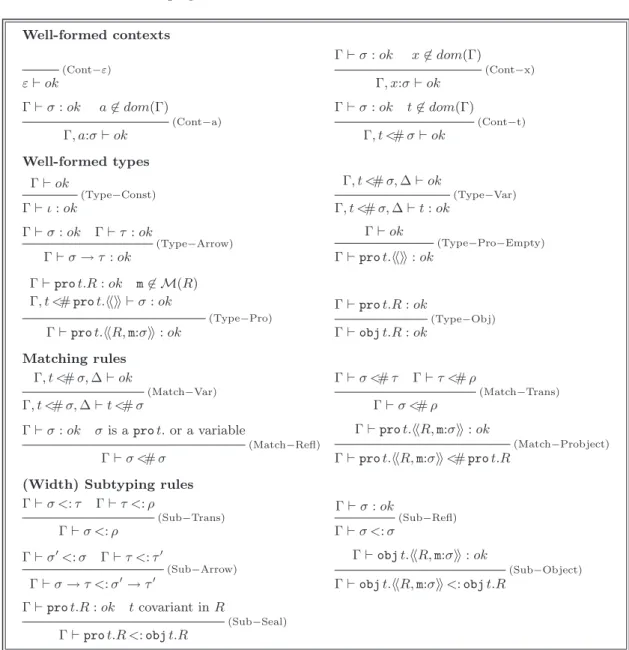
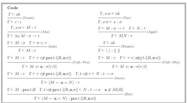
6. A Type System for λOba
In this section, we present a simple type system for λOba, inspired by the systems of Fisher and Mitchell in (Fisher & Mitchell 1995) and Bono and Bugliesi in (Bono & Bugliesi 1999). This type system feature subtyping, which allow method bodies to operate uniformly over all objects having some minimum set of required methods.
6.1. Types
Types are built from type constants, type variables, a function space constructor, and two type abstractions called respectively obj and pro. Moreover, one introduces row of types designed for typing objects with methods.
The type expressions are described as follows. For simplicity we work with a single base type constant ι.
σ, τ ::= ι | t | σ → τ | pro t.R | obj t.R
R, R0 ::= hhii | hhR, m:σii
Here σ and τ are meta-variables ranging over types. R, and R0are meta-variables ranging over rows.
Here are intuitions behind these concepts.
—ι is a constant, base, type.
—A row R is an unordered set of pairs (method label, method type).
—t are type-variables. Type variables play a role in type abstractions (obj or pro) which