HAL Id: hal-00510821
https://hal.archives-ouvertes.fr/hal-00510821
Submitted on 1 Sep 2015
HAL is a multi-disciplinary open access
archive for the deposit and dissemination of
sci-entific research documents, whether they are
pub-lished or not. The documents may come from
teaching and research institutions in France or
abroad, or from public or private research centers.
L’archive ouverte pluridisciplinaire HAL, est
destinée au dépôt et à la diffusion de documents
scientifiques de niveau recherche, publiés ou non,
émanant des établissements d’enseignement et de
recherche français ou étrangers, des laboratoires
publics ou privés.
E. Kyrölä, J. Tamminen, Viktoria Sofieva, Jean-Loup Bertaux, Alain
Hauchecorne, Francis Dalaudier, D. Fussen, F. Vanhellemont, O. Fanton
d’Andon, G. Barrot, et al.
To cite this version:
E. Kyrölä, J. Tamminen, Viktoria Sofieva, Jean-Loup Bertaux, Alain Hauchecorne, et al.. GOMOS O3,
NO2, and NO3 observations in 2002-2008. Atmospheric Chemistry and Physics, European Geosciences
Union, 2010, 10 (16), pp.7723-7738. �10.5194/acp-10-7723-2010�. �hal-00510821�
2Laboratoire Atmosph`eres, Milieux, Observations Spatiales, Universit´e Versailles St.-Quentin, CNRS-INSU, Verri`eres-le-Buisson, France
3Institut d’A´eronomie Spatiale de Belgique, Brussels, Belgium 4ACRI-ST, Sophia Antipolis, France
5European Space Research Institute (ESRIN), European Space Agency, Frascati, Italy
Received: 18 December 2009 – Published in Atmos. Chem. Phys. Discuss.: 1 February 2010 Revised: 9 June 2010 – Accepted: 17 August 2010 – Published: 20 August 2010
Abstract. The Global Ozone Monitoring by Occulta-tion of Stars (GOMOS) instrument onboard the European Space Agency’s ENVISAT satellite measures ozone, NO2, NO3, H2O, O2, and aerosols using the stellar occultation method. Global coverage, good vertical resolution and the self-calibrating measurement method make GOMOS obser-vations a promising data set for building various climatolo-gies and time series. In this paper we present GOMOS night-time measurements of ozone, NO2, and NO3during six years 2002–2008. Using zonal averages we show the time evolu-tion of the vertical profiles as a funcevolu-tion of latitude. In order to get continuous coverage in time we restrict the latitudi-nal region to 50◦S–50◦N. Time development is analysed by fitting constant, annual and semi-annual terms as well as so-lar and QBO proxies to the daily time series. Ozone data cover the stratosphere, mesosphere and lower thermosphere (MLT). NO2and NO3data cover the stratosphere. In addi-tion to detailed analysis of profiles we derive total column distributions using the fitted time series.
The time-independent constant term is determined with a good accuracy (better than 1%) for all the three gases. The median retrieval accuracy for the annual and semi-annual term varies in the range 5–20%. For ozone the annual terms dominate in the stratosphere giving early winter ozone max-ima at mid-latitudes. Above the ozone layer the annual terms change the phase which results in ozone summer maximum up to 80 km. In the MLT the annual terms dominate up
Correspondence to: E. Kyr¨ol¨a
(erkki.kyrola@fmi.fi)
to 80 km where the semiannual terms start to grow. In the equatorial MLT the semi-annual terms dominate the temporal evolution whereas in the mid-latitude MLT annual and semi-annual terms compete evenly. In the equatorial stratosphere the QBO dominates the time development but the solar term is too weak to be determined. In the MLT above 85 km the solar term grows significantly and ozone has 15–20% dependence on the solar cycle. For NO2 below 32 km the annual summer maxima dominates at mid-latitudes whereas in the equatorial region a strong QBO prevails. In northern mid-latitudes a strong solar term appears in the upper strato-sphere. For NO3the annual variation dominates giving rise to summer maxima. The NO3 distribution is controlled by temperature and ozone.
1 Introduction
GOMOS (Global Ozone Monitoring by Occultation of Stars) is a stellar occultation instrument onboard the ENVISAT satellite (see Bertaux et al. (1991, 2000, 2004); Bertaux et al. (2010); Kyr¨ol¨a et al. (2004); ESA (2001), http://envisat.esa. int/handbooks/gomos/ and other articles of this special vol-ume). GOMOS measurements start at altitude of 130 km and the first few measurements are used to determine star’s undis-turbed spectrum (the reference spectrum). The horizontal transmission spectra are calculated from the star spectra mea-sured through the atmosphere and the reference spectrum. The integration time is 0.5 s, which gives the altitude sam-pling resolution of 0.5–1.6 km depending on the tangent al-titude and the azimuth angle of the measurement. GOMOS
measures during day and night but only nighttime measure-ments have been validated so far.
The spectral ranges of GOMOS detectors are 248–690 nm, 755–774 nm, and 926–954 nm, which make it possible to retrieve vertical profiles of O3, NO2, NO3, H2O, O2, and aerosols. In this work we are concentrating on O3, NO2, NO3 and they are retrieved from the UV-visible spectral range 248–690 nm. The retrieved ozone profiles have 2 km ver-tical resolution below 30 km and 3 km above 40 km. NO2 and NO3have 3 km vertical resolution at all altitudes. The details of the retrieval algorithms and data quality are dis-cussed in Kyr¨ol¨a et al. (2010); Tamminen et al. (2010), http: //envisat.esa.int/dataproducts/gomos and in other articles of this special volume.
GOMOS measurements provide a possibility to investi-gate nighttime global vertical distributions of ozone, NO2, and NO3distributions from the tropopause up to the meso-sphere and even to the lower thermomeso-sphere (ozone only). We have earlier presented ozone distributions for the year 2003 in Kyr¨ol¨a et al. (2006) and NO2, and NO3 distributions in Hauchecorne et al. (2005). Now we can extend the analy-sis over the six year period 2002–2008. The longer period makes it possible to study various natural cycles in the data. We will retrieve annual and semi-annual variation as well as variation due to the solar cycle and the quasi-biennial oscil-lation (QBO). The period consider is, however, too short to study anthropogenic trends in data. Besides providing new insights to the atmospheric dynamics and chemistry, the anal-ysis gives valuable information about the GOMOS product quality and the consistency of the data sets.
In Sect. 2 we present the selection of data used for anal-ysis. The method used in the time series fitting is detailed in Sect. 3. Sections 4–6 show results for ozone, NO2 and NO3, respectively. For each gas we present first time evolu-tion of profiles using monthly and 20-degree latitudinal av-erages. The times series fitting is based on daily data and 10-degree latitudinal averages. We show the time-averaged constant term and various cyclic components of the vertical profiles. We also calculate vertical column densities using the time series fits of profiles.
2 Selection of data
Like for all new instruments, a lot of effort has been tar-geted to GOMOS geophysical validation and comparisons with results from other satellite instruments. GOMOS data validation activity has been carried out since the summer of 2002. A comprehensive validation of ozone profiles against ground-based and balloon-borne instruments has been pre-sented in Meijer et al. (2004). Results show that in dark limb GOMOS ozone profile data agree very well with the correlative data: between 14 and 64 km altitude their differ-ences show only a small (2.5–7.5%) negative bias (GOMOS smaller than the correlative data) with a standard deviation of
11–16% (19–63 km). From comparisons with other satellite instrument we can mention, for example, the extensive ACE validation study in Dupuy et al. (2009) and the GOMOS-MIPAS comparison including also mesospheric altitudes in Verronen et al. (2005). GOMOS NO2 measurements have been compared with HALOE in Hauchecorne et al. (2005), with MIPAS in Verronen et al. (2009) and with ACE-FTS in Kerzenmacher et al. (2008). For NO3we have validation with a balloon borne instrument in Renard et al. (2008).
In this work we use GOMOS dark limb measurements only by requiring the solar zenith angle at the tangent point to be greater than 107◦. In Fig. 1 we have shown the distribution of GOMOS nighttime measurements during 2002–2009. The good coverage of the winter poles and the missing coverage of the summer poles are evident. During May–June 2003 and December–August 2005 GOMOS suffered from a malfunc-tioning of the pointing system. In 2003 this can be seen only as a moderate decrease in the number of measurements but in 2005 a real gap in the measurements was produced. New pointing system related problems appeared during 2009 but this study is restricted to 2002–2008. The instrumental prob-lems of GOMOS have forced to restrict the azimuth range of the pointing system from the original −10◦to 90◦ (mea-sured with respect to the antivelocity vector of ENVISAT) to a window of 20◦with a variable center. These changes mean that the selection of stars has not been constant during the time frame of this study.
The solar zenith angle limit 107◦together with the abil-ity of GOMOS to follow and measure stars outside the or-bital plane of ENVISAT leads to a variation in the local hour of measurements. This is important for measurements of diurnally varying constituents NO2, NO3 and ozone in the MLT. ENVISAT crossing times of the equator are 10:00 and 22:00 local time. GOMOS tangent point local times cover 1.5 h in the equator and 3 h at mid-latitudes as shown in Fig. 2.
To assure the reliability of GOMOS data during the whole time period considered, we have paid special attention to the quality of retrievals from each star individually. In Kyr¨ol¨a et al. (2006) we studied the quality of GOMOS measure-ments during 2003 and found that stars with magnitude weaker than 1.9 (i.e. magnitude larger than) and cooler than 7000 K may easily fail to capture the whole ozone profile 15– 100 km. During the course of time GOMOS S/N-ratios have decreased due to aging of the instrument. We have examined data quality for the 6 year period 2002–2008 and compared, for example, time series formed by individual stars. In or-der to guarantee data quality and consistency over the whole time period considered we have removed all ozone measure-ments from 57 different stars. The temperatures and magni-tudes of these stars fulfill approximately the limits mentioned above. For NO2, and NO3all stars were used without regard of magnitude or temperature of the stars. In all data sets we rejected occultations with the obliquity angle (derived from the angle between the occultation plane and the orbital plane
Fig. 1. Monthly number of dark limb occultations (solar zenith
angle greater than 107◦) in 28 August 2002–8 August 2009 as a function of time and latitude. Measurements have been collected monthly to the 10◦latitudinal grid. Occultations that have ended be-fore the 20 km tangent height or that have the obliquity angle larger than 80◦have been disregarded. The grid cells that have fewer than 2 measurements carry white colour.
of ENVISAT) larger than 80◦. The total number of dark limb
occultations 2002–2008 were then 277 449 for NO2and NO3 and 173 223 for ozone.
In the monthly and daily time series plots and analysis we have adopted the following data gridding:
– Vertical: data is linearly interpolated to a uniform 1 km
grid 15–100 km. Flagged data points are not used in the analysis. Ozone profiles from 57 cool and dim stars were not used in statistical calculations.
– Latitudinal: in monthly time series we have used 20◦
latitudinal bands. In time series analysis we have used 10-degree latitude bands with the exception of the equa-torial belt 10◦S–10◦N. Time series analysis is done for the region 50◦S–50◦N where no seasonal data voids ex-ist.
– Zonal: data are zonally averaged in latitude bands
men-tioned.
– Time: we have used monthly time step to present the
overall behaviour of profiles in time. The time period is 28 August 2002–8 August 2009. In time series analysis daily step is used. The time period is1 September 2002– 31 August 2008.
As a statistical average we have used median as the median is more robust against outliers than the normal mean estima-tor (see Kyr¨ol¨a et al. (2006) for the comparison of the mean,
Fig. 2. Number of occultations as a function of the local time for
GOMOS dark limb occultations (solar zenith angle greater than 107◦) in 2004 for two latitude belts. The red line: 5◦S–5◦N, the blue line: 40◦N–50◦N.
the weighted mean and the median). The uncertainty of the median value is estimated by the formula
1ρ = (q3−q1) 1.349 √ N s π N 2(N − 1) (1)
The quartile distance q3−q1(q3and q1are 75% and 25% percentiles, respectively) has been divided by 1.349 in order to take into account the relationship of the quartile distance to the standard deviation in the normal distribution limit. This scaled quartile distance is also used to measure the variability of data. The last factor, where N is the number of cases, takes into account the inefficiency of the median estimator (see http://mathworld.wolfram.com/StatisticalMedian.html). The minimum number of measurements needed for statis-tical estimation has been set to 5. For smaller number of mea-surements we have ignored the contribution. Typical median number of measurements in the equatorial 20-degree latitude belt is 280 in a month. In a day the corresponding median is 14.
The GOMOS data used for this analysis are produced by the ESA Level 2 operational processor version 5. This sion deviates only slightly from the earlier processor ver-sion 4. The upcoming verver-sion 6 improves the level 1 calibra-tion and implements the so-called full covariance matrix in the spectral inversion. The calibration update may somewhat alleviate the problem with weak and cool stars and then in-crease the number of useful occultations. The full covariance matrix will make the GOMOS error estimates more realistic. In this work we will not use error estimates in analysis. We expect, therefore, that the results obtained in this work can be compared to earlier results and that they remain relevant for future studies using the upcoming processor version.
Fig. 3. Normalised daily proxies (see Eq. 3) as a function of time.
The solar F10.7 cm radio flux (red line) serves a solar proxy. The winds at 10 hPa (solid green line) and 30 hPa (dashed green line) are proxies for the QBO effects.
3 Methods
The time series analysis is based on the fitting the daily me-dian profiles ρ(z,t) (z=altitude, t=time) in each latitude belt with the following model:
ρfit(z,t ) = c(z) + s(z)F10.7(t ) + q1(z)Fqbo10(t ) + q2(z)Fqbo30(t ) + 2 X n=1 (an(z)cos(nwt) + bn(z)sin(nwt )) (2)
where w = 2π/365.25 (1/day). This series includes three geophysical proxies. F10.7, the solar 10.7 cm radio flux, is a proxy for solar influence on the middle atmosphere. Fqbo10 and
Fqbo30 are the equatorial winds at 10 hPa and at 30 hPa, respec-tively. They are proxies for quasi-biennial effects (QBO). The observational basis for these proxies are discussed in Harris et al. (1999) and WMO (2007) and references therein. We have normalised the solar and QBO terms in Eq. (2) as
f (t ) =2(f (t) − hf (t)i)/(fmax−fmin) (3) where <> represents average over the six year period con-sidered. Normalised proxies are shown in Fig. 3. Note that for the solar term many authors have adopted a convention where changes are measured in one hundred F10.7 units. F10.7 values have decreased from about 180 units in 2002 to 67 units in 2008 i.e., the change is 113 units. Note also that the declining phase of the solar cycle during our data pe-riod has been unusually long. A time delay in a QBO proxy is often introduced for non-equatorial regions. Using two QBO terms, that are almost in quadrature in time (see Fig. 3), makes the time delay unnecessary.
The purpose of the normalisation in Eq. 3 is to make all the coefficients directly comparable with each other. Moreover, by selecting the time period to be exactly whole number of years (6 years 1 September 2002–31 August 2008) the time average of the series ρfitequals to the constant term. Notice that this average differs from the time average of the mea-sured GOMOS data because of gaps in data whereas the time series in Eq. (2) is defined for all the days of the time period considered.
A linear trend term is manifestly missing from the time series Eq. (2). Looking at the solar proxy in Fig. 3 we can see that in the time period considered, the time smoothed solar proxy deviates only slightly from a linear trend. The linear and solar term are, therefore, highly similar. We have selected the solar term over the linear term as the former has more structure in time and therefore stronger “fingerprint”.
In the case of stratospheric ozone the annual term in Eq. (2) can be justified because of the annual variation of the Brewer-Dobson meridional circulation and the annual vari-ation of the solar insolvari-ation. In the mesosphere the merid-ional pole-to-pole circulation changes the direction semi-annually and this is one justification for the semi-annual term in Eq. (2). Adding higher harmonic terms does not signifi-cantly improve the quality of fits.
Instead of the harmonic terms we could have used physi-cally more direct proxies. For example, the strength of the Brewer-Dobson circulation has been explained by the esti-mate of the Eliassen-Palm flux at 100 hPa in Dhomse et al. (2006). We tested this possibility but no additional benefit in fitting was obtained.
Retrieving the time series coefficients is done by using the weighted least squares fitting. The weights are the estimated data covariances for each day. In our analysis we use the number densities (at geometrical altitudes) because they are the natural units for densities retrieved from GOMOS mea-surements. We have also experimented with fitting mixing ratio data but no clear improvements in the fit quality were evident. The monthly time series of the mixing ratios on pressure surfaces can be found at http://fmilimb.fmi.fi/.
The quality of the fitting has first been checked visu-ally. More quantitative measures used are the error estimates from fitting. We have checked the autocorrelation functions for the fitting residuals and found them reasonably close to normal. We have also studied χ2 values and the coeffi-cient of determination R2 (see http://en.wikipedia.org/wiki/ Coefficient of determination). The last mentioned quantity has turned out to be the most useful measure. The signifi-cance of the time series components have been investigated by fitting various component configurations and inspecting the changes in the R2values. As a final check for results we have done fitting using also monthly time series. Monthly and daily fits give generally fitting components that are very close to each other.
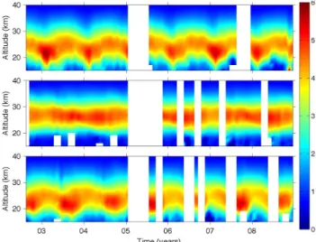
Fig. 4. Monthly ozone number density in the stratosphere in three
latitude belts as a function of time and altitude. The density is scaled by 1012cm−3. The time covered is 1 August 2002–31 December 2008. Latitude belts: 30◦N–50◦N (top), 10◦S–10◦N (middle), 30◦S–50◦S (bottom). White space in the panels means that there are not enough data available.
4 Ozone
In Fig. 4 we show the time development of the ozone num-ber density in the stratosphere based on monthly medians and 20-degree latitude belts. The evident variation in time is a seasonal cycle at mid-latitudes. During winter and spring the ozone layer moves downwards and quite a sharp peak pro-trudes towards the tropopause in early winter at the northern mid-latitudes. At the same time ozone densities in the layer increase. At southern mid-latitudes these changes are some-what smoother. These changes are consequences of the large scale Brewer-Dobson circulation of ozone from the equato-rial region to high-latitudes. During summer the ozone layer retreats to higher altitudes. The equatorial ozone layer re-mains relatively stable in time.
Figure 5 shows the time development of ozone in the MLT. A clear semi-annual variation of the second ozone maximum appears at all latitudes. The strongest variation and high-est values are seen in the equatorial distribution with max-ima around the equinox times. At higher latitudes the semi-annual peaks seem to be slightly merging through the winter season. The spring peak seems to form at somewhat higher altitude than the fall peak. During the six years of observa-tions the second maximum seems to be weakening.
The overall latitudinal distribution of ozone at 20 km and at 90 km is shown in Fig. 6. The 20 km surface dissects the ozone layer at mid-latitudes and shows the winter-spring ozone maxima but lies below the ozone layer at the equator. The 90 km surface is inside the second ozone layer at all lati-tudes. During the equinox times the second ozone maximum appears at all latitudes, other times it is concentrated more above the winter pole.
Fig. 5. Monthly ozone number density in the MLT in three latitude
belts as a function of time and altitude. The density is scaled by 108cm−3. The time covered is 1 August 2002–31 December 2008. Latitude belts: 30◦N–50◦N (top), 10◦S–10◦N (middle), 30◦S– 50◦S (bottom).
In Fig. 7 we have shown the relative variability of the ozone monthly time series as a function of time and altitude in three latitude belts. We have subtracted the variability of the estimated retrieval errors of GOMOS data. Below 20 km the variability is high but otherwise the overall variability in the stratosphere is low. The median over latitudes and times in the stratosphere is 5.5% (the same average for retrieval errors is 0.6%). Somewhat higher variability appears at mid-latitudes during the winter times. In the MLT a very high variability can be seen around the ozone minimum 75–85 km and reduced variability around the ozone maximum at 90 km. The median over latitudes and times in the MLT is 19% (the same average for retrieval errors is 1%).
How does the diurnal variation of ozone affect these re-sults? In Fig. 8 we have shown the diurnal variation of ozone at three altitudes as estimated from the NCAR ROSE model (see also SABER results in Huang et al., 2008). The diurnal variation can safely be ignored in the stratosphere but not in the MLT. The diurnal variation affects the variability through the local hour sampling distributions shown in Fig. 2. The variability caused by these distributions is 2–4% at 90 km. The difference in the mean of the two sampling distributions is below 3% at 90 km.
In order to get a more quantitative view into the systematic variations of the ozone distribution in time, we have carried out a time series analysis of the ozone number density pro-files in the latitude range 50◦S–50◦N. The latitudinal limits are such that there are no seasonal gaps in data (as would be in polar areas). Figure 9 shows an example of the time se-ries fitting to the ozone number density data at 90 km in the latitudinal belt 40◦N–50◦N. The figure also includes the cor-responding fit residual and the individual fitting components.
Fig. 6. Monthly ozone number density at 90 km (upper panel, scaled
by 108cm−3) and 20 km (lower panel, scaled by 1012cm−3) as a function of time and latitude in 1 August 2002–31 December 2008.
Fig. 7. Monthly ozone variability in 15–100 km in three latitude
belts as a function of time and altitude. The variability shown is the quartile distance of data subtracted by the quartile distance of the retrieval errors (the factor 1/1.349 of Eq. (1) included). The values are relative to the median values and in %. Latitude belts: 30◦N– 50◦N (top), 10◦S–10◦N (middle), 30◦S–50◦S (bottom).
The solar, QBO and harmonic terms are in relative units with respect to the constant term (not shown in this figure). Fig-ure 9 shows that the fit at 90 km is able to follow reasonably well the large semi-annual oscillation of ozone and it also shows a declining mean ozone content from the solar term in the MLT. The fit fails to replicate the high ozone values seen above the sinusoidal maxima (for high values of ozone in the MLT, see Smith et al., 2008).
The constant term profiles (c(z) in Eq. 2) at different lat-itudes are shown in Fig. 10 and Fig. 11. The constant term has a low median fitting uncertainty of 0.16%. The profiles
Fig. 8. Ozone number density as a function of the local time at three
altitudes. Densities are calculated using the NCAR ROSE model in 5◦S–5◦N. The number densities are scaled by the maximum values reached at a given altitude.
Fig. 9. An example of the O3number density fitting at 90 km in 40◦N–50◦N. Time axis unit is day. In the upper panel GOMOS measurements are shown by the blue dots and the fit by the black line. The residual is shown by red dots. All three scaled by scaled by 108cm−3. In the lower panel the identifications are: Annual (a1and b1contributions): dashed red, Semi-annual (a2and b2 con-tributions): dashed blue, QBO 1 (q1and q2contributions): solid green, solar (s): solid magenta. The components have been scaled by a constant coefficient and given in %. The constant term itself has not been shown.
show the stratospheric main ozone layer and the secondary ozone layer in the MLT. Besides the two maxima, the deep ozone minimum around 80 km is noteworthy. The strato-spheric and MLT contributions are nearly symmetric with respect to the equator. The main peak altitude is latitude
Fig. 10. The constant factor c(z) in the O3time series as a function of latitude and altitude. Upper panel: MLT with the scale 108cm−3. Lower panel: Stratosphere with the scale 1012cm−3.
Fig. 11. The O3constant factor c(z) as a function of altitude for several latitude belts. The panel in left shows constant profiles 15– 100 km at different latitudes. The upper right panel shows the same profiles in the MLT (values scaled by 108) and the lower right panel in the stratosphere (values scaled by 1012).
dependent whereas the MLT structure (minimum and the sec-ond maximum) is almost independent of latitude. If we cal-culate the total ozone from the constant term in the range 15– 100 km the ozone column is 244 Dobson units in the equa-tor, 264 Dobson units in south mid-latitudes and 271 Dobson units in north mid-latitudes.
The annual, semi-annual, QBO and solar amplitudes for the stratosphere are shown in Fig. 12 and for the MLT in Fig. 13. The relative uncertainties of the harmonic
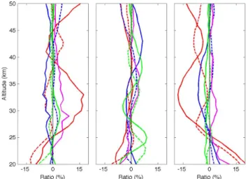
compo-Fig. 12. Fitting components for ozone as a function of altitude in
three latitude belts in the stratosphere. All amplitudes have been given as a ratio between the original amplitude in Eq. (2) and the the constant term c(z) in Eq. (2) and given in %. Line identifi-cations: annual (a1 and b1): solid and dashed red, respectively, Semi-annual (a2and b2): solid and dashed blue, respectively, QBO 10 hPa (q1) and 30 hPa (q2): solid and dashed green, respectively, solar (s): solid magenta. The zero value line has been shown by a thin black line. Left: 50◦S–40◦S, Middle: 10◦S–10◦N, Right: 40◦N–50◦N.
nents vary considerably as a function of altitude. The median (over latitudes 50◦S–50◦N and altitudes 20–100 km)
uncer-tainty values are in the range 5–15%. The annual amplitudes (a1and b1) dominate over the semi-annual ones (a2and b2). Below 25 km the annual amplitude increases (absolute value) at all latitudes towards the tropopause. At the equator the in-crease takes place below the ozone layer but at mid-latitudes it is inside the ozone layer. The two components (a1and b1) have the same sign and this leads to the winter maxima of ozone in both hemispheres. The amplitude is larger at north-ern than at southnorth-ern latitudes. The second increase of the an-nual amplitude a1takes place at mid-latitudes in 30–35 km giving rise a summer maximum. There is an interesting deep minimum at mid-latitudes in the annual oscillation around 25 km.
In the MLT below 70 km the first (a1) annual term domi-nates at mid-latitudes all other amplitudes being small. The annual amplitude (absolute value) reaches 75% in south and 50% in north at 75 km. Notice that these amplitudes have opposite signs when compared to the annual amplitudes in the ozone layer below 25 km. They lead to summer maxima. The signs are changed again when the mid-latitude annual terms go through zero at 80 km and reaches new maxima of 85% (south) and 60% (north) around 83 km. The semi-annual amplitudes start to increase after 75 km at all latitudes. In the equator the first semi-annual component (a2) rapidly increases up to 85% at 82 km and then slowly decreases at higher altitudes. At 90 km it is 50% and dominates over other
Fig. 13. Fitting components as a function of altitude in three latitude
belts in the MLT. All amplitudes have been given as a ratio between the original amplitude in Eq. (2) and the the constant term c(z) in Eq. (2) and given in %. Line identifications: Annual (a1and b1): solid and dashed red, respectively. Semi-annual (a2and b2): solid and dashed blue, respectively, solar (s): solid magenta. The QBO values are not shown. The zero value line has been shown by a thin black line. Left: 50◦S–40◦S, Middle: 10◦S–10◦N, Right: 40◦N– 50◦N.
amplitudes. This gives maximum ozone density in the begin-ning of April and October. At mid-latitudes around the sec-ond maximum the annual and semi-annual amplitudes have nearly the same (absolute) value. The density shows a mix of annual and semi-annual cycles. An example was shown in Fig. 9.
The minor components of the time series are the solar and QBO terms. We have studied changes in the R2-values for the fitting time series Eq. (2) where solar, QBO or both are eliminated. In the equatorial area up to 40 km the two QBO terms considerably improve the quality of the fitting. The solar term improves the fits only in the MLT above 85 km (equator and north) and above 90 km (south). Everywhere else the solar and QBO contributions to the fits are small.
In the equatorial stratosphere QBO terms have relatively large values of 8–9% between 20 and 40 km. The median uncertainty (over altitudes) of the QBO terms is 3.5%. The QBO shows two cell structure with maxima around 25 km and 38 km. In the MLT the solar term grows with altitude reaching 20–25% at 100 km with the median relative uncer-tainty of 8–10% above 85 km. At the second ozone maxi-mum the solar contribution is almost zero in the SH but 17– 19% at the equator and northern mid-latitudes.
The fit for the ozone times series is defined for all times during the 6 years period, for all latitudes 50◦S–50◦N and for all altitudes 15–100 km. Therefore, it is possible to cal-culate various vertical column distributions. Fig. 14 shows the ozone columns in 15–100 km and in 80–100 km. The “total” column shows clearly the mid-latitude ozone
winter-Fig. 14. The daily vertical partial ozone columns as a function of
time and latitude. The columns are calculated from the time se-ries. The upper panel gives the partial column in 80–100 km and the lower panel the partial column in 15–100 km. The unit in both figures is Dobson unit (2.69 × 10¹⁶molecules cm−2).
spring maxima and low ozone values in the equator. The lowest values in this altitude limited column distribution are seen around 15◦N during winter. In the MLT the semi-annual variation prevails everywhere with largest columns at the equator. The overall structure replicates the zigzag pat-tern already seen in Fig. 6. The equatorial ozone in the MLT shows a decreasing trend.
The results obtained above can be compared with the ear-lier results in literature. The limitation of the present data set to the declining part of the very peculiar solar cycle 23 must be remembered when results are compared with time series covering several solar cycles. Results about the annual and semi-annual cycles are hard to find as the time series are usu-ally deseasonalized before the regression analysis. In Perliski et al. (1989) the authors show annual and semi-annual am-plitudes in the stratosphere based on SBUV 1978–1987 mea-surements and a two-dimensional photochemical model. The corresponding amplitudes (of mixing ratios) from GOMOS and SBUV are quite similar.
The physical and chemical processes behind the strato-spheric variations of ozone are discussed in detail in Perliski et al. (1989) and in Ko et al. (1989) and summarised in Brasseur and Solomon (2005) and in Dessler (2000). The explanation for the strong semiannual signal in the MLT has been sought from the semi-annual change of the pole-to-pole meridional circulation and from the semi-annual variation of the diurnal tide (see Smith (2004) and references therein). The former affects the H2O amount and therefore the cat-alytic reactions of hydrogen with ozone. The solar tide af-fects O-related ozone chemistry (production and loss) and temperature. In the stratosphere and MLT the chemical mod-elling predicts anticorrelation of temperature and ozone.
Fig. 15. Correlations of the monthly ozone median densities with
the monthly median temperatures (from ECMWF) as a function of altitude. Left: 30◦S–50◦S, Middle: 10◦S–10◦N, Right: 30◦N– 50◦N. Line identifications: DJF: blue, MAM: red, JJA: green, SON: cyan.
The correlation of GOMOS monthly ozone and monthly temperature (from ECMWF) in the stratosphere is shown in Fig. 15 for four seasons and three latitude regions. In the equatorial region the correlation is for all seasons positive below 30 km and changes then to negative. This change can be understood as the transition from the region of dynami-cal control to the region of chemidynami-cal control (see Brasseur and Solomon, 2005). Mid-latitude correlations show similar transitions but not in so uniform way.
There are many studies on solar cycle effects on strato-spheric ozone profiles. Reviews of the results can be found in Harris et al. (1999) and in WMO (2007). In our quite a short data set it was not possible to extract the solar response in the stratosphere. Using longer satellite data series the so-lar effect has been successfully retrieved in Randel and Wu (2007); Soukharev and Hood (2006); Jones et al. (2009). In the MLT the solar cycle has been estimated only by vari-ous model simulations. In Marsh et al. (2007) the WACCM3 simulations indicate 50% increase in the ozone mixing ratio from the solar minimum to the solar maximum. In our case the changes in number densities at the second maximum are at most 20%.
Many studies have dealt with QBO effects in stratospheric ozone profiles. Reviews of the results can be found in Har-ris et al. (1999) and in WMO (2007). GOMOS results agree about the two cell structure in the equatorial stratosphere dis-cussed, for example, in Randel and Wu (2007).
5 NO2
The nighttime distribution of NO2 from GOMOS measure-ments is shown in Fig. 16. A clear annual cycle is visible at
Fig. 16. Monthly NO2number density in the stratosphere in three latitude belts in 2002–2008 as a function of time and altitude. The density is scaled by 109cm−3. The time covered is 1 August 2002– 31 December 2008. Latitude belts: 30◦N–50◦N (top), 10◦S– 10◦N (middle), 30◦S–50◦S (bottom).
mid-latitudes. The “NO2layer” around 30 km starts to ex-pand in early winter mainly towards the tropopause but also in a lesser amount to higher altitudes. The maximum extent is reached during midsummer. After the maximum the layer contracts from the lower side while the upper boundary still increases. The minimum of the layer is reached in late fall. In the equatorial band a weak semi-annual cycle prevails. The variability of the NO2distribution (not shown) is around 20% at the maximum 30 km. The median over latitudes and times in the stratosphere is 25% (the same average for retrieval er-rors is 13%). The diurnal variation of NO2and NO3from the NCAR ROSE model is shown in Fig. 17. The variability due to the diurnal variation is 3–6%. The difference in the mean of the two sampling distributions is below 4%.
In Fig. 18 we show an example of the time series fitting in the 40◦N–50◦N latitude band at 30 km. In this case
GO-MOS data are reasonably well fitted with the annual term dominating.
The constant term in Figs. 19 and 20 shows a robust dis-tribution around 30 km. The median fitting uncertainty is 0.4%. The maximum values are reached at mid-latitudes. The overall distribution is quite symmetric with respect to the equator. The partial column 20–50 km from the con-stant term peaks at mid-latitudes with 5.3×1015cm−2 in south and 5.2×1015cm−2 in north. The equator column is 3.9×1015cm−2.
The fitting components are shown in Fig. 21. At mid-latitudes the annual amplitude (a1) is around 10–15% at the maximum (30 km) and grows to 60–80% below the maximum. The annual variation has been analysed from the chemistry and dynamics viewpoints in Bracher et al. (2005) and Brohede et al. (2007). At the equator the largest
Fig. 17. NO2 number density vs. local time at 30 km and NO3 number density vs local time at 40 km. The number densities are scaled by the maximum values reached at a given altitude. Results are from the NCAR ROSE model in 5◦S–5◦N.
Fig. 18. An example of the NO2number density fitting at 30 km in the 40◦N–50◦N latitude band. Time axis unit is day. In the upper panel GOMOS measurements are shown by the blue dots and the fit by the black line. The residual is shown by red dots. All three scaled by scaled by 109cm−3. In the lower panel the identifications are: annual (a1and b1contributions): dashed red, Semi-annual (a2and
b2contributions): dashed blue, QBO 1 (q1and q2contributions): solid green, solar (s): solid magenta. The components have been scaled by a constant coefficient and given in %. The constant term itself has not been shown.
harmonic is semi-annual term (a2) with the amplitude of 6%. The median uncertainty of the harmonics varies 4–12%.
Both the solar and QBO term improve the quality of the NO2fits. The median uncertainties for solar and QBO are in the range of 14–21%. The QBO has a similar nodal struc-ture at the equator as ozone had. The maximum amplitude of
Fig. 19. The constant factor c(z) in the NO2time series as a func-tion of latitude and altitude. The scale is 109cm−3.
Fig. 20. The NO2 constant factor profiles c(z) as a function of altitude for several latitude belts. The profile values are scaled by 109.
the QBO is 18% at the equator around the NO2maximum. A second, smaller peak can be found at 43 km. At mid-latitudes the QBO impact is small. The solar term at the equator shows negative values (i.e. more NO2during the solar minimum) in 25–40 km 10%. At southern and northern latitudes negative values are also seen below 35 km. In south and at the equa-tor the solar term is small in the upper stratosphere but at the northern latitudes the solar term grows to 30% in the upper stratosphere. In Hood and Soukharev (2006) authors anal-yse NOxcontent at altitudes 32–53 km using HALOE results in 1991–2003. They found in the equatorial region negative values of 10% around 35 km and 20% around 50 km. GO-MOS results agree with the first finding but do not show the large solar impact in the upper equatorial stratosphere.
Fig. 21. NO2fitting components as a function of altitude in three latitude belts in the stratosphere. All amplitudes have been given as a ratio between the original amplitude in Eq. (2) and the the con-stant term c(z) in Eq. (2) and given in %. Line identifications: An-nual (a1and b1): solid and dashed red, respectively, Semi-annual (a2and b2): solid and dashed blue, respectively, QBO 10 hPa (q1) and 30 hPa (q2): solid and dashed green, respectively, solar (s): solid magenta. The zero value line has been shown by a thin black line. Left: 50◦S–40◦S, Middle: 10◦S–10◦N, Right: 40◦N–50◦N. Note that the x-axis ranges vary in panels.
Figure 22 shows the NO2total column in 20–50 km. Clear annual summer maxima at mid-latitudes and minimum val-ues in the equatorial region. The maximum regions seem to be slightly inclined on the time-latitude plane with the maxi-mum delayed towards higher latitudes.
6 NO3
The number density distribution of GOMOS NO3 measure-ments is shown in Fig. 23. The “NO3 layer” shows a re-markable extent in vertical with the maximum at 40 km. At the mid-latitudes a clear annual cycle is evident with a clear asymmetry between southern and northern latitudes. The maxima seem to appear at the same time through the layer. The equatorial NO3shows a semi-annual cycle with maxima at the equinox times. The maxima have more variation than the ones at mid-latitudes. The variability of the NO3 dis-tribution (not shown) is around 30% at 40 km. The median variability over latitudes and times in the stratosphere is 56% (the same average for retrieval errors is 36%). The diurnal variation of NO3is shown in Fig. 17. The variability due to the diurnal variation is 2–4%. The difference in the mean of the two sampling distributions is below 3%.
Figure 24 shows a fitting example at 40 km (the number density maximum) at the southern mid-latitudes 40◦S–50◦S. The variation at these latitudes can be explained to a large part by the annual term. The solar and QBO terms are very small.
Fig. 22. The daily vertical partial NO2column in 20–50 km as a function of time and latitude. The column is calculated from the time series and scaled by 1015molecules cm−2.
Fig. 23. Monthly NO3number density in the stratosphere in three latitude belts in 2002–2008 as a function of time and altitude. The density is scaled by 107cm−3. The time covered is 1 August 2002– 31 December 2008. Latitude belts: 30◦N–50◦N (top), 10◦S– 10◦N (middle), 30◦S–50◦S (bottom).
The latitude distribution and profiles of the constant term are shown in Fig. 25 and Fig. 26. The median fitting uncer-tainty is 0.6%. The constant term shows a remarkable anvil shape with a large latitudinal extent at the maximum density region around 40 km and a deep vertical extent around the equator. The distribution is nearly symmetric with respect to the equator. The total column from the constant term 25– 50 km peaks in the equator with the column 34×1012cm−2. At southern mid-latitudes the column is 26×1012cm−2and at northern mid-latitudes 25×1012cm−2.
Fig. 24. An example of the NO3number density fitting at 40 km in 40◦S–50◦S. Time axis unit is day. In the upper panel GOMOS measurements are shown by the blue dots and the fit by the black line. The residual is shown by red dots. All three scaled by scaled by 107cm−3. In the lower panel the identifications are: Annual (a1and b1contributions): dashed red, Semi-annual (a2and b2 con-tributions): dashed blue, QBO 1 (q1and q2contributions): solid green, solar (s): solid magenta. The components have been scaled by a constant coefficient and given in %. The constant term itself has not been shown.
The other time series coefficients are shown in Fig. 27. The annual term (a1) dominates strongly the time evolution outside the equatorial region with the maximum amplitude of 60% in south and 40% in north. In the equatorial region the semi-annual amplitude is around 15% dominating the varia-tion. The median uncertainties of the harmonic components are 6–20%. The inclusion of the QBO improves the fit only in the equatorial region and has at the NO3maximum 10% amplitude. The solar term does not make difference in the fit even if the contributions in Fig. 27 are large. The median estimated uncertainty for the solar term is 30% and for the QBO 27–54%.
Figure 28 shows the total NO3column in 25–50 km. The total column shows clear semi-annual variation in the equato-rial region and annual summer maxima with strongest max-ima at the southern latitudes.
As pointed in Hauchecorne et al. (2005), the NO3 density is controlled by a temperature sensitive reaction NO2+O3→NO3+O2. The correlation between temperature and NO3 is shown in Fig. 29 The correlation in 30–45 km is high except the at mid-latitudes during winter when very little NO3can be found.
During nighttime ozone and NO3 are nearly in equilib-rium and their ratio can be approximated by (Eq. (5.173) in Brasseur and Solomon, 2005)
ρNO3
ρO3
= b9 ρb12
(4)
Fig. 25. The NO3constant term c(z) of the time series as a function of latitude and altitude. The scale is 107cm−3.
Fig. 26. The NO3constant term c(z) as a function of altitude for several latitude belts. The profile values are scaled by 107.
where ρ is the neutral density. The coefficient b9is the rate coefficient for NO2+O3→NO3+O2and b12for NO3+NO2 +M → N2O5+M. Both depend on temperature. We have cal-culated the ratio Eq. (4) using GOMOS monthly data for the same latitude belts used in Figs. 4 and 23. Taking the median over times the experimental and theoretical value are inside 20% from each other below 40 km for all latitude regions but deviate strongly at higher altitudes.
Fig. 27. NO3fitting components as a function of altitude in three latitude belts in the stratosphere. All amplitudes have been given as a ratio between the original amplitude in Eq. (2) and the the con-stant term c(z) in Eq. (2) and given in %. Line identifications: An-nual (a1and b1): solid and dashed red, respectively, Semi-annual (a2and b2): solid and dashed blue, respectively, QBO 10 hPa (q1) and 30 hPa (q2): solid and dashed green, respectively, solar (s): solid magenta. The zero value line has been shown by a thin black line. Left: 50◦S–40◦S, Middle: 10◦S–10◦N, Right: 40◦N–50◦N. Note that the x-axis ranges vary in panels.
Fig. 28. The daily vertical partial NO3column in 25–50 km as a function of time and latitude The column is calculated from the time series and scaled by 1012molecules cm−2.
7 Conclusions
In this paper we have analysed 6 years of GOMOS mea-surements of O3, NO2, and NO3. We constructed monthly and daily time series for the vertical profiles using GOMOS nighttime measurements. The daily time series were first ex-amined for consistency by comparing time series from
dif-Fig. 29. Correlations of the monthly GOMOS NO3median den-sities with the monthly median temperatures (from ECMWF) as a function of altitude. Left: 30◦S–50◦S, Middle: 10◦S–10◦N, Right: 30◦N–50◦N. Line identifications: DJF: blue, MAM: red, JJA: green, SON: cyan.
ferent stars. For ozone we found 57 stars that were not able to provide consistent ozone profile data in 15–100 km for the whole 6 year period. For NO2and NO3all stars were found useful in the 20–50 km height range. The latitudinal area analysed was restricted to 50◦S–50◦N to get continu-ous time coverage. The polar regions were not investigated as night (or day) measurements alone cannot provide con-tinuous coverage. Studies of GOMOS measurements of O3, NO2, and NO3in the polar regions can be found, for exam-ple, in Verronen et al. (2006), Sepp¨al¨a et al. (2007), T´etard et al. (2009), and Sofieva et al. (2009).
We analysed the daily time series of O3, NO2, and NO3 profiles by fitting the series by a time independent constant term, annual and semi-annual terms, a solar proxy and two QBO proxies. We did not include a linear trend term in our model because the length of the data set turned out to be too short to distinguish the linear variation and the solar varia-tion. The fitting has been based on daily median values in latitude belts. The fit was also performed using monthly val-ues and the results were found to be close to daily results. The importance of the various terms was examined by calcu-lating R2and χ2values for fits. For all three constituents the constant term, annual and semi-annual term were easily de-termined. For ozone the QBO terms were found important in the equatorial stratosphere. Because of the shortness of the period considered, the fitting of the solar term did not make significant improvement in the stratospheric ozone time se-ries but in the MLT we found large declining trends from the solar contribution. For NO2both the QBO and the so-lar term improved the fits at all latitudes. For NO3only the QBO improved the fit. The NO3 distribution below 40 km was found to be controlled to a large extent by temperature and ozone. Notice that a paper by Hauchecorne et al. (2010)
in this special volume investigates the role of QBO and tem-perature in tropical ozone, NO2and NO3distributions mea-sured by GOMOS.
In our analysis we have not taken into account the spe-cial local hour sampling patterns of GOMOS. This omission may affect the latitude distributions of MLT ozone and strato-spheric NO2and NO3. The diurnal effect could be addressed by classifying data according to the local hour of measure-ment but this obviously reduces the statistical accuracy of results.
The GOMOS data set presented here can provide new valuable nighttime climatologies for O3, NO2, and NO3 profiles. Preliminary yearly climatological data sets can be found at http://fmilimb.fmi.fi/. For stratospheric ozone there are already several climatologies like Fortuin and Kelder (1998); Brunner et al. (2006); Randel and Wu (2007); McPeters et al. (2007); Hassler et al. (2008). In Kyr¨ol¨a et al. (2006) we have made comparison of GOMOS 2003 results with the Fortuin-Kelder results but the comparison of the present 6 year GOMOS data set with the aforementioned cli-matologies requires a new study. The GOMOS MLT ozone data climatology is unique but a similar data set can be con-structed from SABER measurements. Comparisons of MLT data with models will be very interesting as many processes in the MLT are still much more uncertain than the ones in the stratosphere. For NO2 there exist a recent climatology of Brohede et al. (2007, 2008). The NO3GOMOS data set is unique as most of the other instruments need sunlight to work and there is very little NO3during daytime.
Acknowledgements. We want to thank both the referees for useful comments. We want to thank also Anne Smith, Dan Marsh, Martin Kaufman, Leif Backman, Marko Laine, Laura Th¨olix and Esko Kyr¨o for valuable discussions.
Edited by: M. Van Roozendael
References
Bertaux, J. L., Megie, G., Widemann, T., Chassefiere, E., Pellinen, R., Kyr¨ol¨a, E., Korpela, S., and Simon, P.: Monitoring of Ozone Trend by Stellar Occultations: The GOMOS Instrument, Adv. Space Res., 11, 237–242, 1991.
Bertaux, J. L., Kyr¨ol¨a, E., and Wehr, T.: Stellar Occultation Tech-nique for Atmospheric Ozone Monitoring: GOMOS on Envisat, Earth Observation Quarterly, 67, 17–20, 2000.
Bertaux, J. L., Hauchecorne, A., Dalaudier, F., Cot, C., Kyr¨ol¨a, E., Fussen, D., Tamminen, J., Leppelmeier, G. W., Sofieva, V., Has-sinen, S., d’Andon, O. F., Barrot, G., Mangin, A., Th´eodore, B., Guirlet, M., Korablev, O., Snoeij, P., Koopman, R., and Fraisse, R.: First results on GOMOS/Envisat, Adv. Space Res., 33, 1029– 1035, 2004.
Bertaux, J. L., Kyr¨ol¨a, E., Fussen, D., Hauchecorne, A., Dalaudier, F., Sofieva, V., Tamminen, J., Vanhellemont, F., Fanton d’Andon, O., Barrot, G., Mangin, A., Blanot, L., Lebrun, J. C., P´erot, K., Fehr, T., Saavedra, L., and Fraisse, R.: Global ozone monitoring
by occultation of stars: an overview of GOMOS measurements on ENVISAT, Atmos. Chem. Phys. Discuss., 10, 9917–10076, doi:10.5194/acpd-10-9917-2010, 2010.
Bracher, A., Sinnhuber, M., Rozanov, A., and Burrows, J. P.: Using a photochemical model for the validation of NO2satellite mea-surements at different solar zenith angles, Atmos. Chem. Phys., 5, 393–408, doi:10.5194/acp-5-393-2005, 2005.
Brasseur, G. P. and Solomon, S.: Aeronomy of the Middle Atmo-sphere, Springer, Dordrecht, 3rd revised and enlarged edn., 2005. Brohede, S., McLinden, C. A., Berthet, G., Haley, C. S., Murtagh, D., and Sioris, C. E.: A stratospheric NO2 climatology from Odin/OSIRIS limb-scatter measurements, Can. J. Phys., 85, 1253–1274, doi:10.1139/P07-141, 2007.
Brohede, S., McLinden, C. A., Urban, J., Haley, C. S., Jonsson, A. I., and Murtagh, D.: Odin stratospheric proxy NOy mea-surements and climatology, Atmos. Chem. Phys., 8, 5731–5754, doi:10.5194/acp-8-5731-2008, 2008.
Brunner, D., Staehelin, J., Maeder, J. A., Wohltmann, I., and Bodeker, G. E.: Variability and trends in total and vertically re-solved stratospheric ozone based on the CATO ozone data set, Atmos. Chem. Phys., 6, 4985–5008, doi:10.5194/acp-6-4985-2006, 2006.
Dessler, A.: The chemistry and physics of stratospheric ozone, Aca-demic Press, 2000.
Dhomse, S., Weber, M., Wohltmann, I., Rex, M., and Burrows, J. P.: On the possible causes of recent increases in northern hemispheric total ozone from a statistical analysis of satellite data from 1979 to 2003, Atmos. Chem. Phys., 6, 1165–1180, doi:10.5194/acp-6-1165-2006, 2006.
Dupuy, E., Walker, K. A., Kar, J., Boone, C. D., McElroy, C. T., Bernath, P. F., Drummond, J. R., Skelton, R., McLeod, S. D., Hughes, R. C., Nowlan, C. R., Dufour, D. G., Zou, J., Nichitiu, F., Strong, K., Baron, P., Bevilacqua, R. M., Blumenstock, T., Bodeker, G. E., Borsdorff, T., Bourassa, A. E., Bovensmann, H., Boyd, I. S., Bracher, A., Brogniez, C., Burrows, J. P., Catoire, V., Ceccherini, S., Chabrillat, S., Christensen, T., Coffey, M. T., Cortesi, U., Davies, J., De Clercq, C., Degenstein, D. A., De Mazi`ere, M., Demoulin, P., Dodion, J., Firanski, B., Fis-cher, H., Forbes, G., Froidevaux, L., Fussen, D., Gerard, P., Godin-Beekmann, S., Goutail, F., Granville, J., Griffith, D., Ha-ley, C. S., Hannigan, J. W., H¨opfner, M., Jin, J. J., Jones, A., Jones, N. B., Jucks, K., Kagawa, A., Kasai, Y., Kerzenmacher, T. E., Kleinb¨ohl, A., Klekociuk, A. R., Kramer, I., Kllmann, H., Kuttippurath, J., Kyr¨ol¨a, E., Lambert, J.-C., Livesey, N. J., Llewellyn, E. J., Lloyd, N. D., Mahieu, E., Manney, G. L., Mar-shall, B. T., McConnell, J. C., McCormick, M. P., McDermid, I. S., McHugh, M., McLinden, C. A., Mellqvist, J., Mizutani, K., Murayama, Y., Murtagh, D. P., Oelhaf, H., Parrish, A., Petelina, S. V., Piccolo, C., Pommereau, J.-P., Randall, C. E., Robert, C., Roth, C., Schneider, M., Senten, C., Steck, T., Strandberg, A., Strawbridge, K. B., Sussmann, R., Swart, D. P. J., Tarasick, D. W., Taylor, J. R., T´etard, C., Thomason, L. W., Thompson, A. M., Tully, M. B., Urban, J., Vanhellemont, F., Vigouroux, C., von Clarmann, T., von der Gathen, P., von Savigny, C., Waters, J. W., Witte, J. C., Wolff, M., and Zawodny, J. M.: Validation of ozone measurements from the Atmospheric Chemistry Experi-ment (ACE), Atmos. Chem. Phys., 9, 287–343, doi:10.5194/acp-9-287-2009, 2009.
spheric NO2 and NO3observed by Global Ozone Monitoring by Occultation of Stars (GOMOS)/Envisat in 2003, J. Geophys. Res., 110, D18301, doi:10.1029/2004JD005711, 2005.
Hauchecorne, A., Bertaux, J. L., Dalaudier, F., Keckhut, P., Lemen-nais, P., Bekki, S., Marchand, M., Lebrun, J. C., Kyr¨ol¨a, E., Tamminen, J., Sofieva, V., Fussen, D., Vanhellemont, F., Fan-ton d’Andon, O., Barrot, G., Blanot, L., Fehr, T., and Saavedra de Miguel, L.: Response of tropical stratospheric O3, NO2and NO3to the equatorial Quasi-Biennial Oscillation and to tempera-ture as seen from GOMOS/ENVISAT, Atmos. Chem. Phys. Dis-cuss., 10, 9153–9171, doi:10.5194/acpd-10-9153-2010, 2010. Hood, L. L. and Soukharev, B. E.: Solar induced variations of odd
nitrogen: Multiple regression analysis of UARS HALOE data, Geophys. Res. Lett., 33, L22805, doi:10.1029/2006GL028122, 2006.
Huang, F. T., Mayr, H. G., Russell, J. M., Mlynczak, M. G., and Reber, C. A.: Ozone diurnal variations and mean profiles in the mesosphere, lower thermosphere, and stratosphere, based on measurements from SABER on TIMED, Journal of Geo-physical Research (Space Physics), 113, A04307, doi:10.1029/ 2007JA012739, 2008.
Jones, A., Urban, J., Murtagh, D. P., Eriksson, P., Brohede, S., Ha-ley, C., Degenstein, D., Bourassa, A., von Savigny, C., Sonkaew, T., Rozanov, A., Bovensmann, H., and Burrows, J.: Evolu-tion of stratospheric ozone and water vapour time series studied with satellite measurements, Atmos. Chem. Phys., 9, 6055–6075, doi:10.5194/acp-9-6055-2009, 2009.
Kerzenmacher, T., Wolff, M. A., Strong, K., Dupuy, E., Walker, K. A., Amekudzi, L. K., Batchelor, R. L., Bernath, P. F., Berthet, G., Blumenstock, T., Boone, C. D., Bramstedt, K., Brogniez, C., Brohede, S., Burrows, J. P., Catoire, V., Dodion, J., Drummond, J. R., Dufour, D. G., Funke, B., Fussen, D., Goutail, F., Grif-fith, D. W. T., Haley, C. S., Hendrick, F., H¨opfner, M., Huret, N., Jones, N., Kar, J., Kramer, I., Llewellyn, E. J., L´opez-Puertas, M., Manney, G., McElroy, C. T., McLinden, C. A., Melo, S., Mikuteit, S., Murtagh, D., Nichitiu, F., Notholt, J., Nowlan, C., Piccolo, C., Pommereau, J.-P., Randall, C., Raspollini, P., Ri-dolfi, M., Richter, A., Schneider, M., Schrems, O., Silicani, M., Stiller, G. P., Taylor, J., T´etard, C., Toohey, M., Vanhellemont, F., Warneke, T., Zawodny, J. M., and Zou, J.: Validation of NO2and NO from the Atmospheric Chemistry Experiment (ACE), At-mos. Chem. Phys., 8, 5801–5841, doi:10.5194/acp-8-5801-2008, 2008.
M., Koopman, R., Saavedra, L., Snoeij, P., and Fehr, T.: Night-time ozone profiles in the stratosphere and mesosphere by the Global Ozone Monitoring by Occultation of Stars on Envisat, J. Geophys. Res., 111, D24306, doi:10.1029/2006JD007193, 2006. Kyr¨ol¨a, E., Tamminen, J., Sofieva, V., Bertaux, J. L., Hauchecorne, A., Dalaudier, F., Fussen, D., Vanhellemont, F., Fanton d’Andon, O., Barrot, G., Guirlet, M., Mangin, A., Blanot, L., Fehr, T., Saavedra de Miguel, L., and Fraisse, R.: Retrieval of atmospheric parameters from GOMOS data, Atmos. Chem. Phys. Discuss., 10, 10145–10217, doi:10.5194/acpd-10-10145-2010, 2010. Marsh, D. R., Garcia, R. R., Kinnison, D. E., Boville, B. A., Sassi,
F., Solomon, S. C., and Matthes, K.: Modeling the whole at-mosphere response to solar cycle changes in radiative and geo-magnetic forcing, J. Geophys. Res.-Atmos., 112, D23306, doi: 10.1029/2006JD008306, 2007.
McPeters, R. D., Labow, G. J., and Logan, J. A.: Ozone clima-tological profiles for satellite retrieval algorithms, J. Geophys. Res.-Atmos., 112, D05308, doi:10.1029/2005JD006823, 2007. Meijer, Y. J., Swart, D. P. J., Allaart, M., Andersen, S. B., Bodeker,
G., Boyd, Braathena, G., Calisesia, Y., Claude, H., Dorokhov, V., von der Gathen, P., Gil, M., Godin-Beekmann, S., Goutail, F., Hansen, G., Karpetchko, A., Keckhut, P., Kelder, H. M., Koele-meijer, R., Kois, B., Koopman, R. M., Lambert, J.-C., Leblanc, T., McDermid, I. S., Pal, S., Kopp, G., Schets, H., Stubi, R., Suortti, T., Visconti, G., and Yela, M.: Pole-to-pole validation of ENVISAT/GOMOS ozone profiles using data from ground-based and balloon-sonde measurements, J. Geophys. Res., 109, D23305, doi:10.1029/2004JD004834, 2004.
Perliski, L. M., Solomon, S., and London, J.: On the interpretation of seasonal variations of stratospheric ozone, Planet. Space Sci., 37, 1527–1538, doi:10.1016/0032-0633(89)90143-8, 1989. Randel, W. J. and Wu, F.: A stratospheric ozone profile data set
for 1979-2005: Variability, trends, and comparisons with column ozone data, J. Geophys. Res.-Atmos., 112, D06313, doi:10.1029/ 2006JD007339, 2007.
Renard, J., Berthet, G., Brogniez, C., Catoire, V., Fussen, D., Goutail, F., Oelhaf, H., Pommereau, J., Roscoe, H. K., Wet-zel, G., Chartier, M., Robert, C., Balois, J., Verwaerde, C., Au-riol, F., Franc¸ois, P., Gaubicher, B., and Wursteisen, P.: Vali-dation of GOMOS-Envisat vertical profiles of O3, NO2, NO3, and aerosol extinction using balloon-borne instruments and anal-ysis of the retrievals, Journal of Geophysical Research (Space Physics), 113, A02302, doi:10.1029/2007JA012345, 2008.
Sepp¨al¨a, A., Verronen, P. T., Clilverd, M. A., Randall, C. E., Tam-minen, J., Sofieva, V. F., Backman, L., and Kyr¨ol¨a, E.: Arc-tic and AntarcArc-tic polar winter NOx and energetic particle pre-cipitation in 2002–2006, Geophys. Res. Lett., 34, L12810, doi: 10.1029/2007GL029733, 2007.
Smith, A. K.: Physics and chemistry of the mesopause region, J. Atmos. Sol.-Terr. Phys., 66, 839–857, 2004.
Smith, A. K., Marsh, D. R., Russell, J. M., Mlynczak, M. G., Martin-Torres, F. J., and Kyr¨ol¨a, E.: Satellite observations of high nighttime ozone at the equatorial mesopause, J. Geophys. Res.-Atmos., 113, D17312, doi:10.1029/2008JD010066, 2008. Sofieva, V. F., Kyr¨ol¨a, E., Verronen, P. T., Sepp¨al¨a, A., Tamminen,
J., Marsh, D. R., Smith, A. K., Bertaux, J.-L., Hauchecorne, A., Dalaudier, F., Fussen, D., Vanhellemont, F., Fanton d’Andon, O., Barrot, G., Guirlet, M., Fehr, T., and Saavedra, L.: Spatio-temporal observations of the tertiary ozone maximum, At-mos. Chem. Phys., 9, 4439–4445, doi:10.5194/acp-9-4439-2009, 2009.
Soukharev, B. E. and Hood, L. L.: Solar cycle variation of strato-spheric ozone: Multiple regression analysis of long-term satel-lite data sets and comparisons with models, J. Geophys. Res.-Atmos., 111, D20314, doi:10.1029/2006JD007107, 2006. Tamminen, J., Kyr¨ol¨a, E., Sofieva, V. F., Laine, M., Bertaux,
J.-L., Hauchecorne, A., Dalaudier, F., Fussen, D., Vanhelle-mont, F., Fanton-d’Andon, O., Barrot, G., Mangin, A., Guirlet, M., Blanot, L., Fehr, T., Saavedra de Miguel, L., and Fraisse, R.: GOMOS data characterization and error estimation, At-mos. Chem. Phys. Discuss., 10, 6755–6796, doi:10.5194/acpd-10-6755-2010, 2010.
T´etard, C., Fussen, D., Bingen, C., Capouillez, N., Dekemper, E., Loodts, N., Mateshvili, N., Vanhellemont, F., Kyr¨ol¨a, E., Tam-minen, J., Sofieva, V., Hauchecorne, A., Dalaudier, F., Bertaux, J.-L., Fanton d’Andon, O., Barrot, G., Guirlet, M., Fehr, T., and Saavedra, L.: Simultaneous measurements of OClO, NO2and O3in the Arctic polar vortex by the GOMOS instrument, At-mos. Chem. Phys., 9, 7857–7866, doi:10.5194/acp-9-7857-2009, 2009.
Verronen, P. T., Kyr¨ol¨a, E., Tamminen, J., Funke, B., Gil-L´opez, S., Kaufmann, M., L´opez-Puertas, M., von Clarmann, T., Stiller, G., Grabowski, U., and H¨opfner, M.: A comparison of night-time GOMOS and MIPAS ozone profiles in the stratosphere and mesosphere, Adv. Space Res., 36, 958–966, 2005.
Verronen, P. T., Sepp¨al¨a, A., Kyr¨ol¨a, E., Tamminen, J., Pickett, H. M., and Turunen, E.: Production of odd hydrogen in the meso-sphere during the January 2005 solar proton event, Geophys. Res. Lett., 33, L24811, doi:10.1029/2006GL028115, 2006.
Verronen, P. T., Ceccherini, S., Cortesi, U., Kyr¨ol¨a, E., and Tammi-nen, J.: Statistical comparison of night-time NO2observations in 2003–2006 from GOMOS and MIPAS instruments, Adv. Space Res., 43, 1918–1925, doi:10.1016/j.asr.2009.01.027, 2009. WMO: Scientific Assessment of Ozone Depletion: 2006, Global
Ozone Research and Monitoring Project – Report No. 50, World Meteorological Organization, Geneva, Switzerland, 2007.