HAL Id: hal-00414772
https://hal.archives-ouvertes.fr/hal-00414772
Submitted on 6 Sep 2015
HAL is a multi-disciplinary open access
archive for the deposit and dissemination of
sci-entific research documents, whether they are
pub-lished or not. The documents may come from
teaching and research institutions in France or
abroad, or from public or private research centers.
L’archive ouverte pluridisciplinaire HAL, est
destinée au dépôt et à la diffusion de documents
scientifiques de niveau recherche, publiés ou non,
émanant des établissements d’enseignement et de
recherche français ou étrangers, des laboratoires
publics ou privés.
chemistry-climate models
H. Struthers, G.E. Bodeker, J. Austin, Slimane Bekki, I. Cionni, M. Dameris,
M.A. Giorgetta, V. Grewe, Franck Lefèvre, F. Lott, et al.
To cite this version:
H. Struthers, G.E. Bodeker, J. Austin, Slimane Bekki, I. Cionni, et al.. The simulation of the Antarctic
ozone hole by chemistry-climate models. Atmospheric Chemistry and Physics, European Geosciences
Union, 2009, 9 (17), pp.6363-6376. �10.5194/acp-9-6363-2009�. �hal-00414772�
www.atmos-chem-phys.net/9/6363/2009/ © Author(s) 2009. This work is distributed under the Creative Commons Attribution 3.0 License.
Chemistry
and Physics
The simulation of the Antarctic ozone hole by
chemistry-climate models
H. Struthers1,*, G. E. Bodeker1, J. Austin2, S. Bekki3, I. Cionni1, M. Dameris4, M. A. Giorgetta5, V. Grewe4, F. Lef`evre3, F. Lott6, E. Manzini7,8, T. Peter9, E. Rozanov9,10, and M. Schraner9
1National Institute of Water and Atmospheric Research, Lauder, New Zealand 2Geophysical Fluid Dynamics Laboratory, NOAA, Princeton, New Jersey, USA 3Service d’Aeronomie du CNRS, Institut Pierre-Simon Laplace, Paris, France
4Deutsches Zentrum f¨ur Luft- und Raumfahrt, Institut f¨ur Physik der Atmosph¨are, Oberpfaffenhofen, Wessling, Germany 5Max Planck Institut f¨ur Meteorologie, Hamburg, Germany
6Laboratoire de Meteorologie Dynamique, Paris, France 7Istituto Nazionale di Geofisica e Vulcanologia, Italy
8Centro Euro-Mediterraneo per i Cambiamenti Climatici, Bologna, Italy 9Institute for Atmospheric and Climate Science ETH, Zurich, Switzerland 10PMOD/WRC, Dorfstrasse 33, 7260, Davos Dorf, Switzerland
*now at: the Department of Applied Environmental Science, Stockholm University, Sweden
Received: 17 September 2008 – Published in Atmos. Chem. Phys. Discuss.: 1 December 2008 Revised: 7 July 2009 – Accepted: 14 August 2009 – Published: 3 September 2009
Abstract. While chemistry-climate models are able to repro-duce many characteristics of the global total column ozone field and its long-term evolution, they have fared less well in simulating the commonly used diagnostic of the area of the Antarctic ozone hole i.e. the area within the 220 Dob-son Unit (DU) contour. Two possible reaDob-sons for this are: (1) the underlying Global Climate Model (GCM) does not correctly simulate the size of the polar vortex, and (2) the stratospheric chemistry scheme incorporated into the GCM, and/or the model dynamics, results in systematic biases in the total column ozone fields such that the 220 DU contour is no longer appropriate for delineating the edge of the ozone hole. Both causes are examined here with a view to develop-ing ozone hole area diagnostics that better suit measurement-model inter-comparisons. The interplay between the shape of the meridional mixing barrier at the edge of the vortex and the meridional gradients in total column ozone across the vortex edge is investigated in measurements and in 5 chemistry-climate models (CCMs). Analysis of the simu-lation of the polar vortex in the CCMs shows that the first of the two possible causes does play a role in some models. This in turn affects the ability of the models to simulate the
Correspondence to: H. Struthers
large observed meridional gradients in total column ozone. The second of the two causes also strongly affects the ability of the CCMs to track the observed size of the ozone hole. It is shown that by applying a common algorithm to the CCMs for selecting a delineating threshold unique to each model, a more appropriate diagnostic of ozone hole area can be gen-erated that shows better agreement with that derived from observations.
1 Introduction
The phrase “the ozone hole” is used to describe the severe annual Antarctic spring-time ozone depletion that was first observed more than 25 years ago. The ozone hole is most commonly defined as the region at high southern latitudes en-closed by the 220 DU total column ozone contour (Newman et al., 2004). Diagnostics such as the daily ozone hole area and the annual maximum area are widely reported and are used as general measures of the severity of Antarctic ozone depletion. Time series of annual maximum ozone hole area indicate the gross impact of large changes in stratospheric inorganic chlorine and bromine on Antarctic ozone and daily time series of ozone hole area over a single spring season provide information on conditions in the Antarctic strato-sphere relevant to ozone depletion. The spatial extent of
the ozone hole is an important factor determining Antarc-tic surface ultraviolet (UV) radiation levels and ozone hole diagnostics have been extensively used in the World Me-teorological Organization/United Nations Environment Pro-gramme (WMO/UNEP) ozone assessments (WMO/UNEP, 2003, 2007).
CCMs, capable of simulating the most important pro-cesses involved in the production and destruction of strato-spheric ozone are important tools for predicting the con-sequences of anthropogenic emissions of ozone depleting substances. These models are used for multidecadal pro-jections of future stratospheric change (Austin and Wilson, 2006) but to have confidence in these projections the mod-els must be rigorously assessed (Eyring et al., 2005). This is achieved by comparing simulations of the past evolution of ozone, other trace gas species and dynamics under the varying natural and anthropogenic forcings with observa-tions (Austin et al., 2003; Eyring et al., 2006; Bodeker et al., 2007). Whilst CCMs have shown considerable verisimil-itude in many stratospheric diagnostics they do not, as a group, perform well in comparisons between simulated and observed ozone hole area (Austin et al., 2003; Chipperfield et al., 2003; Eyring et al., 2007; Bodeker et al., 2007). Al-though some models perform well, many CCMs underesti-mate the ozone hole size. The CCM ensemble of simulated ozone hole areas used in the 2006 WMO/UNEP ozone as-sessment exhibits a large spread (see Figs. 6–14, Bodeker et al., 2007). The large scatter in the CCM results leads to a very large uncertainty in the ensemble prediction of the date of the disappearance of the ozone hole.
One possible reason for the inaccurate ozone hole areas simulated by CCMs is that the definition of the ozone hole based on the 220 DU threshold may not be appropriate for some models. The 220 DU contour is useful for defining the ozone hole in observations because it is coincident with the strong meridional gradient in total column ozone demarcat-ing the region of severe ozone depletion. This may not be the case for models with total column ozone biases. An ad-ditional possibility is that the size of the Antarctic circumpo-lar vortex is not accurately simulated. If this is the case the size of the modelled ozone hole is also likely to be in error because, for periods of high halogen loading, the area of se-vere ozone depletion is constrained by the polar vortex edge (Bodeker et al., 2002; Newman et al., 2004).
The primary objective of this paper is to examine how the two factors mentioned above (biases in total column ozone and the size of the circumpolar vortex) affect the simulation of the ozone hole area in five CCMs. The CCMs’ simulation of the position and width of the mixing barrier at the edge of the Antarctic polar vortex is compared with meteorolog-ical reanalyses using a metric that highlights the region of reduced meridional mixing at the edge of the Antarctic po-lar vortex (Bodeker et al., 2002; Wang et al., 2005). This analysis follows the study of Bodeker et al. (2002) (hereafter denoted B2002) who used equivalent latitude zonal means of
ozone and meteorological reanalysis to study the expansion of the Antarctic ozone hole and its encroachment on the ob-served edge of the Antarctic vortex. B2002 used equivalent latitude coordinates to remove the effects of vortex displace-ment and elongation which tend to blur gradients near the vortex edge when taking zonal means in true latitude coor-dinates. Combining the results from the comparison of the polar vortex edge with estimates of the total column ozone biases in the CCMs, two diagnostics of the areal extent of Antarctic ozone loss which preserve the ozone hole concept but allow for a more consistent comparison between models and observations are introduced and discussed.
2 Measurement data sets and vortex diagnostics The ozone measurements used in this study were taken from the National Institute of Water and Atmospheric Research (NIWA) combined total column ozone data-base (Bodeker et al., 2005) which is an update of the data-base used in B2002. The data-base combines satellite-based ozone measurements from four Total Ozone Mapping Spectrome-ter (TOMS) instruments, three different retrievals from the Global Ozone Monitoring Experiment (GOME) instruments, data from four Solar Backscatter Ultra-Violet (SBUV) in-struments and data from the Ozone Monitoring Instrument (OMI). Comparisons with the global ground-based World Ozone and Ultraviolet Data Center (WOUDC) Dobson and Brewer spectrophotometer network have been used to re-move offsets and drifts between the different data sets to pro-duce a global homogeneous total ozone column data set that combines the advantages of good spatial coverage of satellite data with the long-term stability of ground-based measure-ments. For more details see Bodeker et al. (2005).
The meridional impermeability, κ, is defined as the gra-dient of potential vorticity (PV) with respect to equivalent latitude (φe) multiplied by the horizontal wind speed (|V|) on a given potential temperature surface:
κ = dPV dφe
× |V| (1)
To calculate κ, wind, temperature and PV fields on poten-tial temperature surfaces were taken from the National Cen-ters for Environmental Prediction/National Center for Atmo-spheric Research (NCEP/NCAR) reanalyses (Kistler et al., 2001). κ is a purely dynamical construct, rather than being defined based on the distribution of an advected tracer. It can therefore be calculated directly from meteorological re-analyses and compared with the same diagnostic calculated from CCM or GCM output. Meridional transects of equiv-alent latitude zonal mean κ versus equivequiv-alent latitude high-light the position and latitudinal structure of the meridional mixing barrier at the vortex edge (Wang et al., 2005). High values of κ indicate regions of high impermeability and low
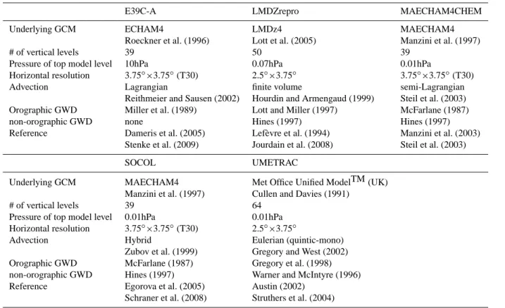
Table 1. Details of the CCMs used.
E39C-A LMDZrepro MAECHAM4CHEM
Underlying GCM ECHAM4 LMDz4 MAECHAM4
Roeckner et al. (1996) Lott et al. (2005) Manzini et al. (1997)
# of vertical levels 39 50 39
Pressure of top model level 10hPa 0.07hPa 0.01hPa
Horizontal resolution 3.75◦×3.75◦(T30) 2.5◦×3.75◦ 3.75◦×3.75◦(T30)
Advection Lagrangian finite volume semi-Lagrangian
Reithmeier and Sausen (2002) Hourdin and Armengaud (1999) Steil et al. (2003) Orographic GWD Miller et al. (1989) Lott and Miller (1997) McFarlane (1987)
non-orographic GWD none Hines (1997) Hines (1997)
Reference Dameris et al. (2005) Lef`evre et al. (1994) Manzini et al. (2003) Stenke et al. (2009) Jourdain et al. (2008) Steil et al. (2003)
SOCOL UMETRAC
Underlying GCM MAECHAM4 Met Office Unified ModelTM (UK)
Manzini et al. (1997) Cullen and Davies (1991)
# of vertical levels 39 64
Pressure of top model level 0.01hPa 0.01hPa Horizontal resolution 3.75◦×3.75◦(T30) 2.5◦×3.75◦
Advection Hybrid Eulerian (quintic-mono)
Zubov et al. (1999) Gregory and West (2002) Orographic GWD McFarlane (1987) Gregory et al. (1998) non-orographic GWD Hines (1997) Warner and McIntyre (1996) Reference Egorova et al. (2005) Austin (2002)
Schraner et al. (2008) Struthers et al. (2004)
meridional mixing. The opposite is true for low (near zero) values of κ.
Daily NCEP/NCAR PV fields (2.5◦ latitude × 2.5◦ lon-gitude resolution) on the 550 K potential temperature sur-face were used to define the equivalent latitude coordinate (B2002). The 550 K surface was chosen for this analysis in accordance with B2002 and close to the 520 K level used by Randel and Wu (1995) in a similar analysis. The po-sition and shape of the equivalent latitude versus κ tran-sects derived from NCEP/NCAR reanalyses change negli-gibly if the 450 K or 475 K isentropes are used rather than the 550 K (see Tilmes et al., 2007). Daily PV versus equiva-lent latitude zonal means were generated and these were used to transform the ozone to an equivalent latitude coordinate. The same procedure was used to generate equivalent latitude zonal means from the CCMs.
3 CCM descriptions
All of the models shown here are fully coupled CCMs that include representations of the feedbacks between the dynam-ics, radiation and chemistry which are present in the real stratosphere. In particular, the way the models simulate the polar vortex will impact the in-situ chemistry which can feed
back on the dynamics through changes in the distribution of radiatively active gases.
A short summary of the salient characteristics of each model is given in Table 1. All of the models have been inter-compared and evaluated against measurements (Eyring et al., 2006, 2007; Bodeker et al., 2007; Austin et al., 2008). The models shown here are a subset of all the models participat-ing in the CCMVal-1 (Chemistry Climate Model Validation, Eyring et al. (2005)) activity of Stratospheric Processes and their Role in Climate (SPARC). Only groups that submitted daily October PV, wind and total column ozone model output to the CCMVal-1 archive are included in this study. Model results in the rest of this paper are listed in alphabetical order. E39C-A (Stenke et al., 2008, 2009) is an upgraded version of the CCM E39C (Dameris et al., 2005, 2006) employing the fully Lagrangian advection scheme ATTILA (Reithmeier and Sausen, 2002) for tracer transport. ATTILA is strictly mass conserving and numerically non-diffusive. Water va-por, cloud water and chemical trace species are advected by ATTILA instead of the operational semi-Lagrangian advec-tion scheme of Williamson and Rasch (1994) which has been used in the previous model version E39C. Extensive changes have been made to the chemistry and advection schemes in the SOCOL model (Schraner et al., 2008) from that presented in Eyring et al. (2006); Bodeker et al. (2007); Eyring et al.
(2007); Austin et al. (2008). Results from SOCOL version 2.0 are used in this study. The chemistry scheme in UME-TRAC has been updated since Austin (2002) and is the same as that used in the AMTRAC model in the study of Austin and Wilson (2006).
The underlying GCM used in MAECHAM4CHEM and SOCOL is the middle atmosphere configuration of ECHAM4 (MAECHAM4) (Manzini et al., 1997). One notable difference in the way MAECHAM4 is configured in MAECHAM4CHEM and SOCOL is that the non-orographic gravity wave scheme in SOCOL has been modified to pro-duce slightly stronger non-orographic gravity wave drag than MAECHAM4CHEM. This adjustment results in some im-provements to the dynamical representation of the strato-sphere in SOCOL with respect to MAECHAM4CHEM (see Figs. 1, 2 and 3 of Eyring et al. (2006)).
All models use the same prescribed changes in ozone de-pleting substances, well mixed greenhouse gases, and strato-spheric aerosol surface area densities as well as observed sea surface temperatures and sea ice lower boundary conditions. These boundary conditions are the same as those used in the so called REF1 CCMVal-1 integrations described in detail in Eyring et al. (2006).
4 Observed dynamical containment of the ozone hole Note that the equivalent latitude mapping of the total col-umn ozone depends on the theta surface of the PV used. For brevity in the rest of the paper, the total column ozone trans-formed to equivalent latitude using the 550 K PV will be sim-ply referred to as the total column ozone. Similarly the 550 K equivalent latitude, zonal mean κ is referred to as κ.
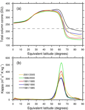
Antarctic ozone depletion typically maximizes during early October (Solomon, 1999). Figure 1 shows the Octo-ber average of daily mean total column ozone (Fig. 1a) and
κ (Fig. 1b) averaged over five year periods. This extends Figs. 2 and 4 of B2002 for a further 5 years beyond 2000. The severity of Antarctic ozone depletion increased from 1981 to 2000 as indicated by the steady decline in the total col-umn ozone poleward of the vortex edge (Fig. 1a). In con-junction with the increased severity of ozone depletion, the equivalent latitude at which the contours cross the 220 DU threshold (denoted by the horizontal dashed line in Fig. 1a) steadily decreased from 1981 to 2000 indicating an increase in area of the ozone hole. These trends reverse for the 2001– 2005 average where the total column ozone within the vor-tex is more than 20 DU greater than the previous five year average and the equivalent latitude of the 220 DU contour has moved poleward by approximately four degrees. The reversal of the ozone trend is not necessarily an indication of the recovery of Antarctic ozone from the effect of reduc-tions in stratospheric halogen concentrareduc-tions. The severity of ozone depletion within the Antarctic polar vortex for a given spring, depends on both chemical and dynamical conditions
Fig. 1. Five year October averages (black: 1981-1985, blue: 1986-1990, red: 1991-1995,
green: 1996-2000, orange: 2001-2005) of daily (a) total column ozone (DU) from NIWA total column ozone data-base and (b) 550K κ (m3s−2K kg−1) from NCEP/NCAR reanalyses.
9
Fig. 1. Five year October averages (black: 1981–1985, blue: 1986–
1990, red: 1991–1995, green: 1996–2000, orange: 2001–2005) of daily (a) total column ozone (DU) from NIWA total column ozone data-base and (b) 550 K κ (m3s−2K kg−1) from NCEP/NCAR re-analyses.
(Huck et al., 2005). The 2002–2005 period was significantly more dynamically active and stratospheric temperatures were higher than previous years (Hoppel et al., 2003; Sinnhuber et al., 2003; Randall et al., 2005).
Figure 1a clearly shows that, for observations over the pe-riod 1980 to 2006, the 220 DU contour delineates the region of severe ozone depletion over the equivalent latitude pole from the higher ozone columns at middle and low latitudes and hence is an appropriate threshold to define the ozone hole edge.
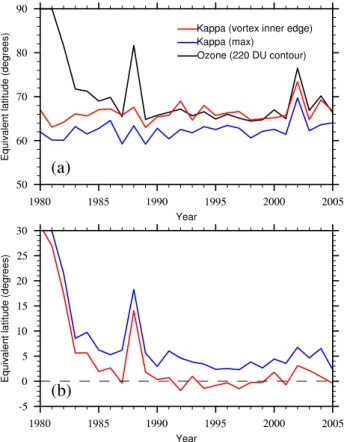
The dynamical edge of the stratospheric polar vortex can been defined in a number of ways (Bodeker et al., 2002; Nash et al., 1996; Tilmes et al., 2006). Here we define the “vortex edge” as the peak in κ and the ’inner vortex edge’ as the min-imum of the second derivative of κ with respect to equivalent latitude (Nash et al., 1996). Figure 2 updates Fig. 3 of B2002, and shows for each year the October average equivalent lat-itude of the 220 DU total column ozone contour, the equiva-lent latitude of the vortex edge and the inner vortex edge. As described by B2002, the equivalent latitude of the polar vor-tex (either the vorvor-tex edge or the inner vorvor-tex edge) changed
Fig. 2. (a) October mean equivalent latitude of the 220 DU contour (black line), the center of
the vortex edge (blue line) and the inner vortex edge (red line). (b) Difference between the equivalent latitude of the 220 DU contour and the center of the vortex edge (blue line), and the inner vortex edge (red line). The ozone results are derived from the NIWA combined data-base and the vortex edge time series are from the NCEP/NCAR reanalyses. See text for definitions of the center of the vortex edge and the inner vortex edge.
28
Fig. 2. (a) October mean equivalent latitude of the 220 DU contour
(black line), the center of the vortex edge (blue line) and the inner vortex edge (red line). (b) Difference between the equivalent lati-tude of the 220 DU contour and the center of the vortex edge (blue line), and the inner vortex edge (red line). The ozone results are derived from the NIWA combined data-base and the vortex edge time series are from the NCEP/NCAR reanalyses. See text for def-initions of the center of the vortex edge and the inner vortex edge.
little from 1980 to 1990, however the area of the ozone hole steadily increased over the same period. The October av-erage ozone hole area has remained relatively constant over the period 1990–2005, except for the anomalous 2002 year which has been attributed to anomalous tropospheric wave forcing (Nishii and Nakamura, 2004). The size of the 1988 ozone hole also appears anomalous in Fig. 2 but without the concomitant change in the position of the vortex edge seen in 2002 (Kanzawa and Kawaguchi, 1990). Differences in the nature of the 1988 and 2002 anomalies demonstrate that comprehensive understanding of the stratospheric response to variations in tropospheric forcing requires the use of pro-cess level diagnostics capable of disentangling the relative roles of dynamics and chemistry.
Figure 2 shows that from approximately 1990, the equiva-lent latitude of the 220 DU total column ozone contour con-sistently lies near the equivalent latitude of the inner vortex edge. This suggests that from approximately 1990, the size
of the ozone hole has largely been constrained by the size of the polar vortex (B2002). This conclusion is supported by Newman et al. (2004) who show that from the early 1990s, the 220 DU ozone hole edge has been located in the weakly mixed zone at the edge of the polar vortex. There were no significant secular trends in the equivalent latitude position of the vortex edge and the inner vortex edge (Fig. 2a) over the period 1980 to 2005, however the size of the ozone hole and the average total column ozone within the inner vortex (Fig. 1a) changed greatly over the same period. From this we conclude that the position of the vortex edge and the in-ner vortex edge, and therefore the size of the circumpolar polar vortex does not change in response to large changes in the concentration of ozone within the vortex. This in spite of the fact that ozone has a strong radiative effect on the strato-sphere and ozone losses have contributed to a delay the aver-age date of the final breakup of the Antarctic vortex (Lange-matz and Kunze, 2006).
5 Dynamical containment of the ozone hole simulated by five CCMs
For the comparison between observations/reanalysis and models, the 1995 to 2000 period was chosen because this is the period where the equivalent effective stratospheric chlo-rine (EESC) (Newman et al., 2007) reaches a maximum. Most of the model simulations used in this work finish in 2000 so this was taken as the end point of the averaging pe-riod.
5.1 Modeled meridional impermeability
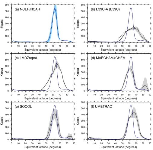
The 5 year average (1995–1999) of the October mean κ de-rived from NCEP/NCAR reanalyses and from the five CCMs are plotted in Fig. 3. The dominant feature in the κ equiv-alent latitude zonal mean is the mixing barrier at the vor-tex edge between approximately 50◦S to 75◦S (Figs. 1b and 3a) This feature is reproduced by all of the CCMs but the details are not well simulated by some of the models. All the models have mixing barriers that are too wide compared to reanalyses, particularly E39C-A, LMDZrepro and UME-TRAC. These three models also simulate vortex edges that are too close to the equivalent latitude pole. These two prob-lems combine such that the position of the inner vortex edge in these models is significantly too close to the equivalent lat-itude pole (see Table 2). Comparisons of the κ from E39C-A and E39C demonstrate the effect of changes in the trace gas advection scheme in these models. κ from both models are similar with E39C-A showing a small improvement com-pared to reanalysis on the equatorward side of the κ peak. The inner edge of the vortex in MAECHAM4CHEM agrees well with the reanalysis results. A second smaller κ peak within the vortex is apparent in the MAECHAM4CHEM re-sults (Fig. 3d). This feature is associated with small, high PV
Table 2. 1995–1999 average equivalent latitude of the maximum in the meridional total column ozone gradient, the vortex edge and the
inner vortex edge from observations, NCEP/NCAR reanalysis and the five CCMs (see Fig. 5). Observations,
NCEP/NCAR E39C-A LMDZrepro MAECHAM4CHEM SOCOL UMETRAC
Maximum ozone gradient 65.4 62.7 62.9 68.1 64.2 63.1
Vortex edge 62.4 67.5 64.1 61.5 62.1 66.4
Inner vortex edge 65.3 74.5 73.6 67.8 68.5 73.7
Fig. 3. Five year (1995-1999) average October κ from (a) NCEP/NCAR reanalyses and (b)
E39C-A (dashed line E39C), (c) LMDZrepro, (d) MAECHAM4CHEM, (e) SOCOL and (f) UME-TRAC. Shading indicates the 1σ standard deviation about the mean. The blue lines are the reanalysis mean overlaid on the model results for comparison.
29
Fig. 3. Five year (1995–1999) average October κ from (a) NCEP/NCAR reanalyses and (b) E39C-A (dashed line E39C), (c) LMDZrepro, (d) MAECHAM4CHEM, (e) SOCOL and (f) UMETRAC. Shading indicates the 1σ standard deviation about the mean. The blue lines are
the reanalysis mean overlaid on the model results for comparison.
events that occur early in October within the polar vortex in some years. These features are also present to a lesser de-gree in the SOCOL fields (Fig. 3e) suggesting that they are generated by the underlying MAECHAM4 GCM. The cause of these features is presently not clear. κ from SOCOL is the only model in agreement with the reanalyses over the latitude range spanning the vortex edge (50◦S to 75◦S).
The shape of the κ peaks from MAECHAM4CHEM and SOCOL are similar. The similarity of κ from MAECHAM4CHEM and SOCOL and the insensitivity of
κto changes in advection scheme (E39C-A/E39C) indicates that the shape of the κ peak derived from CCM output is strongly related to the underlying dynamical model rather than the chemistry or spatial distribution of radiatively ac-tive gases. Further evidence for this conclusion comes from the fact that no significant secular trends in the position of the vortex edge or the inner vortex edge are present in the model results over the 1980–1999 period in accordance with the measurement and reanalysis results discussed in Sect. 4 and shown in Fig. 2.
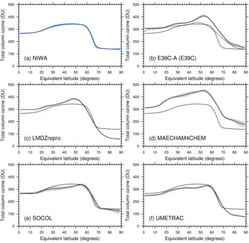
Fig. 4. Five year (1995-1999) average October total column ozone from (a) NIWA
com-bined total column ozone data-base and (b) E39C-A (dashed line E39C), (c) LMDZrepro, (d) MAECHAM4CHEM, (e) SOCOL and (f) UMETRAC. Shading indicates the 1σ standard devia-tion about the mean. The blue lines are the observed mean overlaid on the model results for
comparison.
30
Fig. 4. Five year (1995–1999) average October total column ozone from (a) NIWA combined total column ozone data-base and (b) E39C-A
(dashed line E39C), (c) LMDZrepro, (d) MAECHAM4CHEM, (e) SOCOL and (f) UMETRAC. Shading indicates the 1σ standard deviation about the mean. The blue lines are the observed mean overlaid on the model results for comparison.
As pointed out above, the MAECHAM4CHEM and SO-COL inner vortex edges agree with the reanalysis results (see also Table 2). The other models (E39C-A, LMDZrepro and UMETRAC) simulate inner vortex edges more than 7 de-grees closer to the equivalent latitude pole compared to re-analyses. The poor simulation of the inner vortex edge in these models is in turn expected to impact their ability to ac-curately simulate the ozone hole area.
5.2 Modeled total column ozone
There is a sharp decrease in observed total column ozone at the edge of the vortex between 60◦S and 70◦S equivalent latitude (Fig. 1a and Fig. 4a). This steep gradient highlights the advantage of using equivalent latitude coordinates where the effects of distortion and/or displacement of the vortex are reduced compared to true latitude coordinates (B2002).
Figure 4 compares the measured 1995–1999 October av-erage total column ozone with results from the five CCMs. The total column ozone values from LMDZrepro and UME-TRAC are too low in the vicinity of the equivalent latitude
pole and the MAECHAM4CHEM ozone columns are posi-tively biased over the whole of the southern hemisphere as noted by Steil et al. (2003). The E39C-A total columns also have a positive bias over the whole of the Southern Hemisphere. The shape of the E39C-A total column ozone (Fig. 4b) meridional transect is a small improvement com-pared to results from the E39C model but at the expense of introducing a positive bias at middle and high latitudes. The ozone gradient across the vortex edge is steeper and the large gradients near the vortex edge are more confined in lat-itude in the E39C-A results compared to E39C. Total col-umn ozone from SOCOL version 2.0 shown here is a sig-nificant improvement on the results shown in Eyring et al. (2006, 2007) and are in good agreement with observations, particularly in the tropics and high latitudes.
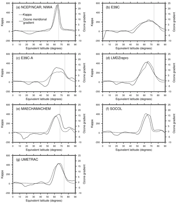
Figure 5 compares the relationship between meridional gradients of total column ozone (solid lines) and κ (dashed lines), averaged between 1995 and 1999. Also plotted is the average position of the inner vortex edge. The shape of the meridional ozone gradients resemble the correspond-ing κ transects both in the observations and the models but
Fig. 5. Comparison of the five year (1995 - 1999) average κ (dashed line) and the
nega-tive of the gradient in total column ozone with respect to equivalent latitude (solid line). (a)
NCEP/NCAR reanalyses and NIWA observation data-base, (b) E39C (c) E39C-A, (d)
LMDZre-pro, (e) MAECHAM4CHEM, (f) SOCOL and (g) UMETRAC. The gray vertical lines indicate the
average position of the inner vortex edge for each model (see Table 2).
31
Fig. 5. Comparison of the five year (1995–1999) average κ (dashed line) and the negative of the gradient in total column ozone with respect
to equivalent latitude (solid line). (a) NCEP/NCAR reanalyses and NIWA observation data-base, (b) E39C (c) E39C-A, (d) LMDZrepro, (e) MAECHAM4CHEM, (f) SOCOL and (g) UMETRAC. The gray vertical lines indicate the average position of the inner vortex edge for each model (see Table 2).
the equivalent latitude position of the maximum ozone gra-dient relative to the κ peak is not well simulated by some of the models. This can be seen in Table 2 which gives the 1995–1999 average equivalent latitude position of the maxi-mum ozone gradient, the vortex edge and inner vortex edge. The equivalent latitude of the maximum ozone gradient in the observations is poleward of the vortex edge by approx-imately three degrees and almost coincident with the inner vortex edge (see also Fig. 2). The position of the maximum ozone gradients are reasonably well simulated by the
mod-els, all being within three degrees of the observations but as discussed in Sect. 5.1 there are significant discrepancies in the position of the vortex edge and inner vortex edge in three of the models (E39C-A, LMDZrepro and UMETRAC).
The fact that the maximum ozone gradient is almost co-incident with the inner vortex edge in observations suggests that the vortex edge acts to confine inner vortex air which is subject to severe ozone depletion. This is consistent with the fact that the meridional temperature gradient drives the zonal wind at the vortex edge (Brasseur and Solomon, 2005) and
the cold temperatures within the vortex drive ozone deple-tion (B2002). Clearly there are deficiencies in the simuladeple-tion of the processes important in determining the position of the maximum ozone gradient relative to the vortex edge in the E39C-A, LMDZrepro and UMETRAC models. The position and magnitude of the ozone gradients in turn are expected to influence the magnitude of the spring ozone resupply into the vortex. For example Lemmen et el. (2006) show through the budget of total and chemical ozone change that the spring ozone resupply is not well simulated in E39C. It is outside the scope of this work to examine what process or processes are causing these models to inaccurately simulate the posi-tion of the maximum ozone gradient relative to the mixing barrier at the vortex edge.
5.3 The simulation of the Antarctic ozone hole using CCMs
Results presented in the above sections demonstrate that the CCMs included in this study have problems with both the simulation of the polar vortex and total column ozone bi-ases. Both factors in turn are expected to affect the ability of these models to accurately simulate the size of the ozone hole, yet these models can simulate severe ozone depletion at high southern latitudes (see for example Fig. 4). Therefore it may be useful to consider ways to formulate diagnostics that allow more consistent measurement/model comparisons which in turn may highlight and improve the exploitation of the useful information contained in the output generated by CCMs.
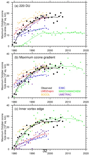
Figure 6a compares the maximum October ozone hole area derived from measurements and the five CCMs using the 220 DU definition of the ozone hole. All the available years of CCM output are plotted in Fig. 6 including projec-tions from MAECHAM4CHEM out to 2020. The 220 DU ozone hole areas from the CCMs shown here are indicative of the results from the full set of CCMs used in the 2006 WMO assessment (Fig. 6-14, Bodeker et al. (2007) and Ta-ble 3 of Eyring et al. (2006)) with the models varying greatly in their ability to simulate the ozone hole size. LMDZrepro and UMETRAC simulate reasonably well the evolution of the 220 DU ozone hole size. The 220 DU ozone hole simu-lated by SOCOL is too large over the 1981–1986 period and MAECHAM4CHEM and E39C significantly underestimate the ozone hole size. Note, no E39C-A results are shown in this section because only 10 years (1990–1999) of model out-put were available and so the onset and development of the ozone hole simulated by this model cannot be studied.
The 220 DU contour may not be appropriate for delin-eating the region of severe ozone depletion for CCMs with total column ozone biases at high latitudes. Two methods of calculating a total column ozone threshold to define the ozone hole consistently across observations and models are discussed below:
Fig. 6. Evolution of the size of the ozone hole from observations (black) and five CCMs (E39C:
blue, LMDZrepro: red, MAECHAM4CHEM: green, SOCOL: orange, UMETRAC: purple). Max-imum October ozone hole area using (a) 220 DU contour, (b) the maxMax-imum ozone gradient threshold, (c) the inner vortex edge threshold (see text for threshold definitions and Table 3 for threshold values). Solid lines are calculated using an 11 year running mean of the annual values.
32
Fig. 6. Evolution of the size of the ozone hole from obser-vations (black) and five CCMs (E39C: blue, LMDZrepro: red, MAECHAM4CHEM: green, SOCOL: orange, UMETRAC: pur-ple). Maximum October ozone hole area using (a) 220 DU contour,
(b) the maximum ozone gradient threshold, (c) the inner vortex edge
threshold (see text for threshold definitions and Table 3 for threshold values). Solid lines are calculated using an 11 year running mean of the annual values.
– Maximum ozone gradient: Calculated by taking the 1995–1999 October average total column ozone at the position of the maximum of the meridional gradient in total column ozone. This ensures that during the period of high halogen loading, the ozone hole threshold se-lected is at the equivalent latitude of the strongest merid-ional ozone gradients (see Fig. 5).
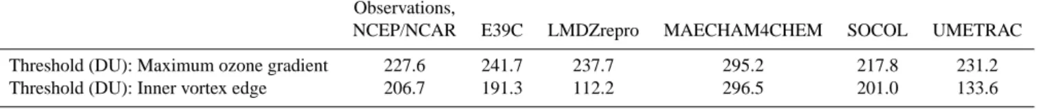
Table 3. Total column ozone thresholds for observations and the 5 CCMs. The thresholds were calculated in two ways as described in the
text based on 1995–1999 averages (also see Fig. 4).
Observations,
NCEP/NCAR E39C LMDZrepro MAECHAM4CHEM SOCOL UMETRAC
Threshold (DU): Maximum ozone gradient 227.6 241.7 237.7 295.2 217.8 231.2
Threshold (DU): Inner vortex edge 206.7 191.3 112.2 296.5 201.0 133.6
– Inner vortex edge: Defined as the total column ozone value at the equivalent latitude of the 1995–1999 Octo-ber average of the inner vortex edge. This threshold was chosen based on the relationship between the position of the inner vortex edge and the maximum of the observed total column ozone gradient seen in Table 2 and follows the conclusions of B2002 that the horizontal extent of the ozone hole is constrained by the inner vortex edge during periods of high halogen loading.
The threshold values determined from observations and re-analyses and the five models are given in Table 3.
The thresholds calculated using the maximum ozone gra-dient method all have relatively similar values and are within 10% of 220 DU except for MAECHAM4CHEM. The inner vortex edge thresholds show a greater spread of values. The three models which perform poorly in simulating the position of inner vortex edge (E39C, LMDZrepro and UMETRAC) all produce low inner vortex edge thresholds. In the case of LMDZrepro and UMETRAC these threshold values are very low reflecting the low bias in total column ozone within the inner vortex in these models. MAECHAM4CHEM has a high inner vortex edge threshold but the value is close to its maximum ozone gradient threshold because the equivalent latitudes of the maximum ozone gradient and the inner vortex edge are nearly coincident (see Table 2). Thus for this model, although there is a large total column ozone bias, the relation-ship between the inner vortex edge and the meridional ozone gradient is accurately simulated. The maximum ozone gra-dient and inner vortex edge thresholds derived from observa-tions and SOCOL are similar and also close to 220 DU.
Maximum October ozone hole size calculated using the maximum ozone gradient threshold are plotted in Fig. 6b. The largest change from the results in Fig. 6a, using the 220 DU threshold, occurs in the MAECHAM4CHEM val-ues which drastically increase and now compare well with observations. The E39C results also show a reasonably large upward shift relative to Fig. 6a. All the other ozone hole ar-eas, including the observed areas show small changes com-pared to Fig. 6a. Based on Fig. 6b, the models (excluding E39C) compare reasonably well with observations in sim-ulating the area enclosed by the steepest meridional ozone gradients, particularly over the 1990–2000 period. LMDZre-pro, SOCOL and UMETRAC simulate an ozone hole that is
too large in the early part of the 1980s using this threshold definition.
Maximum October ozone hole area based in the inner vor-tex edge threshold are plotted in Fig. 6c. This figure mir-rors the results from Table 2 with MAECHAM4CHEM and SOCOL comparing well with observations whereas E39C, LMDZrepro and UMETRAC all manifest ozone hole areas that are significantly too small. MAECHAM4CHEM results shown in Fig. 6a, b and c illustrate how the maximum ozone gradient and inner vortex edge ozone hole definitions can in some cases improve measurement/model comparisons. In this case the model does accurately simulate the areal extent of severe ozone depletion over the Antarctic and its relation-ship to the inner edge of the polar vortex but the bias in total column ozone inherent in the model leads to a poor compar-ison when using the 220 DU ozone hole definition. On the other hand LMDZrepro and UMETRAC compare well with measurements using the 220 DU and maximum ozone gradi-ent definitions but the inner vortex edge results highlight the deficiencies these models have in simulating the confinement of ozone depleted air by the vortex edge. For model evalua-tion, the maximum ozone gradient and the inner vortex edge definitions can be considered complimentary. The maximum ozone gradient definition provides a consistent methodology for evaluating the area of severe ozone depletion over the Antarctic. The inner vortex edge definition provides infor-mation on model fidelity with respect to the size of the vortex and degree of isolation of inner vortex air from mid-latitudes.
6 Discussion and conclusions
The area of the ozone hole is an important diagnostic of se-vere ozone depletion over Antarctica. The CCMs used in the 2006 WMO/UNEP ozone assessment did not perform well as a group in simulating the size of the ozone hole (defined by the 220 DU contour). In general there was a large spread in the Bodeker et al. (2007) results and the multi-model ensem-ble mean underestimates the ozone hole size. Two possiensem-ble reasons for the poor comparison between models and obser-vations are (1) model total column ozone biases mean that the 220 DU contour is not appropriate for some models, (2) the models incorrectly simulate the size of the polar vortex. The extent of the polar vortex limits the area of severe ozone
depletion and thus determines the ozone hole size during the period of high halogen loading.
Simulation of the position and width of the region of re-duced meridional mixing at the edge of the polar vortex was examined here using results from five of the CCMs used in the 2006 WMO/UNEP assessment. The comparisons with results from reanalyses were mixed, some models perform-ing reasonably well whereas others poorly simulate the posi-tion and width of the mixing barrier at the edge of the polar vortex. Three of the models studied here simulate the po-sition of the inner vortex more than 7 degrees closer to the equivalent latitude pole than reanalyses. This in turn affects the ability of these models to accurately simulate the area over which severe ozone depletion takes place.
Total column ozone values from the models were com-pared with measurements to determine any total column ozone biases. As with the simulation of the polar vortex, the total column ozone comparisons vary with some models performing relatively well whereas others manifest large to-tal column ozone biases (both positive and negative). Toto-tal column ozone biases present in the models studied here can affect the ozone hole area calculated using the 220 DU con-tour threshold because the 220 DU concon-tour may not coincide with the region of high meridional gradients in total column ozone near the edge of the polar vortex.
Two methods of calculating a total column ozone thresh-old to define the ozone hole have been examined. For mod-els with large total column ozone biases, using a consistent definition of the ozone threshold can lead to better agree-ment between observed and modelled ozone hole area and can highlight deficiencies in model simulations of the polar vortices. Using the maximum ozone gradient to define the ozone hole threshold leads to reasonable agreement between observations and the five CCMs studied here (Fig. 6b), al-though the E39C model still produces an ozone hole that is significantly too small. Although the maximum ozone gradi-ent definition can be applied consistgradi-ently across observations and models, this method does not provide information about the relative position of the ozone gradients with respect to the position of the vortex edge and therefore cannot be used by itself, to probe the accuracy of CCMs representation of the known coupling between chemical ozone loss and dynamics at the vortex edge. The inner vortex edge definition of the ozone hole threshold can be used to highlight deficiencies in the simulation of the position of the vortex edge in models. It is unclear why in some models, the maximum ozone gra-dients do not coincide with the inner vortex edge as observed in the real atmosphere. Two possible reasons are: (1) insuffi-cient isolation of the vortex, and (2) cold temperature biases leading to an overestimation of in-situ chemical ozone loss in the vortex collar region. Further research is required to examine the possible role these and other factors play in de-termining the relationship between the ozone hole area and the vortex area in CCMs.
Maximum October ozone hole results from SOCOL com-pare well with observations over the period 1990–1999 us-ing all three definitions of the ozone hole (220 DU, max-imum ozone gradient, inner vortex edge) (Fig. 6) which reflects the fact that this model simulates the shape of κ (Fig. 3) and the zonal mean total column ozone (Fig. 4) well. After correcting for the total column ozone bias, the MAECHAM4CHEM ozone hole areas also compare well with observations (Fig. 6b and c). SOCOL and MAECHAM4CHEM results indicate that the current gen-eration of CCMs are capable of accurately simulating the large scale structure of the total column ozone field in the vicinity of the Antarctic vortex edge and its relationship to the underlying dynamics. Using alternative definitions of the ozone hole which remove the effects of total column ozone biases in the CCMs can lead to a greatly improved compari-son with observations and more consistency between models but it should be kept in mind that although agreement with observations can be achieved, significant biases still exist and must be acknowledged.
A possible source of uncertainty arises through the deter-mination of the position of the vortex edge. The vortex edge and the inner vortex edge calculated using NCEP/NCAR re-analyses are insensitive to potential temperature surface used within the range 450 K to 550 K but this is not necessarily the case for CCMs. Indeed Tilmes et al. (2007) show that the position of the vortex edge in the WACCM CCM varies from approximately 62◦S to 58◦S between 550 K and 450 K. Fur-ther study is required to determine how best to relate the po-sition of the vortex edge to the total column ozone in CCMs. Problems with the simulation of the size of the polar vor-tex are expected to affect parameters/fields other than ozone that are also used in model evaluations. The obvious exam-ple is the area of polar stratospheric cloud formation which may be significantly underestimated in some models. Model evaluations that use polar diagnostics related to absolute area should keep this in mind. Comparisons between observations and models near the edge of the polar vortex may be similarly affected.
Acknowledgements. We would like to thank D. Smale (NIWA) for the SOCOL and H. Garny (DLR) for the E39C-A output used in this study. The LMDz-REPRO, MAECHAM4CHEM and the DLR group acknowledges the support of the SCOUT-O3 Integrated Project which is funded by the European Commission. H. S. would like to acknowledge the NIWA high performance computing facility for their support in completing the UMETRAC simulations used in this work and Jill Scott for her assistance. The CCM SOCOL development was supported by the ETH Poly-Projects “VSGC I and II” and by the Swiss National Science Foundation (grant SCOPES IB7320-110884). This work was supported by the New Zealand Foundation for Research, Science and Tech-nology under contract C01X0703. The authors would like to acknowledge the ACP editors and the two anonymous referees for their contribution to improving the original manuscript of this paper. Edited by: W. Lahoz
References
Austin, J.: A three-dimensional coupled chemistry-climate model simulation of past stratospheric trends, J. Atmos. Sci., 59, 218– 232, 2002.
Austin, J., Shindell, D., Beagley, S. R., Br¨uhl, C., Dameris, M., Manzini, E., Nagashima, T., Newman, P., Pawson, S., Pitari, G., Rozanov, E., Schnadt, C., and Shepherd, T. G.: Uncertainties and assessments of chemistry-climate models of the stratosphere, Atmos. Chem. Phys., 3, 1–27, 2003,
http://www.atmos-chem-phys.net/3/1/2003/.
Austin, J. and Wilson, R. J.: Ensemble simulations of the de-cline and recovery of stratospheric ozone, J. Geophys. Res., 111, D16314, doi:10.1029/2005JD006907, 2006.
Austin, J, Tourpali, K., Rozanov, E., Akiyoshi, H., Bekki, S., Bodeker, G., Br¨uhl, C., Butchart, N., Chipperfield, M., Deushi, M., Fomichev, V. I., Giorgetta, M. A., Gray, L., Kodera, K, Lott, F., Manzini, E., Marsh, D., Matthes, K., Nagashima, T., Shibata, K., Stolarski, R. S., Struthers, H., and Tian W.: Coupled chemistry climate model simulations of the solar cy-cle in ozone and temperature, J. Geophys. Res., 113, D11306, doi:10.1029/2007JD009391, 2008.
Bodeker, G. E., Struthers, H. A., and Connor, B. J.: Dynamical Containment of Antarctic Ozone Depletion, Geophys. Res. Lett., 29(7), 1098, doi:10.1029/2001GL014206, 2002.
Bodeker, G. E., Shiona, H., and Eskes, H.: Indicators of Antarctic ozone depletion, Atmos. Chem. Phys., 5, 2603–2615, 2005, http://www.atmos-chem-phys.net/5/2603/2005/.
Bodeker, G. E., and Waugh, D. W. (lead authors) Akiyoshi, H., Braesicke, P., Eyring, V., Fahey, D. W., Manzini, E., Newchurch, M. J., Portmann, R. W., Robock, A., Shine, K. P., Steinbrecht, W., and Weatherhead, E. C.: The ozone layer in the 21st century, Chapter 6, in: Scientific Assessment of Ozone Depletion: 2006, Global Ozone Research and Monitoring Project, Report No. 50, 572 pp., Geneva, Switzerland, 2007.
Brasseur, G. P. and Solomon, S.: Aeronomy of the Middle Atmo-sphere, 3rd Edn., Springer, Dordrecht, The Netherlands, 2005. Chipperfield, M. P., and Randel, W. J. (lead authors) Bodeker, G.
E., Dameris, M., Fioletov, V. E., Friedl, R. R., Harris, N. R. P., Logan, J. A., McPeters, R. D., Muthama, N. J., Peter, T., Shepherd, T. G., Shine, K. P., Solomon, S., Thomason, L. W., and Zawodny, J. W.: Global Ozone: Past and Future, Chapter 4, in: Scientific Assessment of Ozone Depletion: 2002, Global Ozone Research and Monitoring Project, Tech. Rep. Report No. 47, Geneva, Switzerland, 2003.
Cullen, M. and Davies, T.: Conservative split-explicit integration scheme with fourth-order horizontal advection, Q. J. Roy. Me-teor. Soc., 117, 993–1002, 1991.
Dameris, M., Grewe, V., Ponater, M., Deckert, R., Eyring, V., Mager, F., Matthes, S., Schnadt, C., Stenke, A., Steil, B., Br¨uhl, C., and Giorgetta, M. A.: Long-term changes and variability in a transient simulation with a chemistry-climate model employing realistic forcing, Atmos. Chem. Phys., 5, 2121–2145, 2005, http://www.atmos-chem-phys.net/5/2121/2005/.
Dameris, M., Matthes, S., Deckert, R., Grewe, V., and Ponater, M.: Solar cycle effect delays onset of ozone recovery, Geophys. Res. Lett., 33, L03806, doi:10.1029/2005GL024741, 2006.
Egorova, T., Rozanov, E., Zubov, V., Manzini, E., Schmutz, W., and Peter, T.: Chemistry-climate model SOCOL: a validation of the present-day climatology, Atmos. Chem. Phys., 5, 1557–1576,
2005,
http://www.atmos-chem-phys.net/5/1557/2005/.
Eyring, V., Harris, N. R. P., Rex, M., Shepherd, T. G., Fahey, D. W., Amanatidis, G. T., Austin, J., Chipperfield, M. P., Dameris, M., Forster, P. M., Gettelman, A., Graf, H-F., Nagashima, T., Newman, P. A., Pawson, S., Prather, M. J., Pyle, J. A., Salawitch, R. J., Santer, B. D., and Waugh, D. W.: A strategy for process-oriented validation of coupled chemistry-climate models, B. Am. Meteorol. Soc., 86, 1117–1133, 2005.
Eyring, V., Butchart, N., Waugh, D. W., Akiyoshi, H., Austin, J., Bekki, S., Bodeker, G. E., Boville, B. A., Br¨uhl, C., Chipper-field, M. P., Cordero, E., Dameris, M., Deushi, M., Fioletov, V. E., Frith, S. M., Garcia, R. R., Gettelman, A., Giorgetta, M. A., Grewe, V., Jourdain, L., Kinnison, D. E., Mancini, E., Manzini, E., Marchand, M., Marsh, D. R., Nagashima, T., Newman, P. A., Nielsen, J. E., Pawson, S., Pitari, G., Plummer, D. A., Rozanov, E., Schraner, M., Shepherd, T. G., Shibata, K., Stolarski, R. S., Struthers, H., Tian, W., and Yoshiki, M: Assessment of tem-perature, trace species, and ozone in chemistry-climate model simulations of the recent past, J. Geophys. Res., 111, D22308, doi:10.1029/2006JD007327, 2006.
Eyring, V., Waugh, D. W., Bodeker, G. E., Cordero, E., Akiyoshi, H., Austin, J., Beagley, S. R., Boville, B. A., Braesicke, P., Br¨uhl, C., Butchart, N., Chipperfield, M. P., Dameris, M., Deckert, R., Deushi, M., Frith, S. M., Garcia, R. R., Gettelman, A., Giorgetta, M. A., Kinnison, D. E., Mancini, E., Manzini, E., Marsh, D. R., Matthes, S., Nagashima, T., Newman, P. A., Nielsen, J. E., Paw-son, S., Pitari, G., Plummer, D. A., Rozanov, E., Schraner, M., Scinocca, J. F., Semeniuk, K., Shepherd, T. G., Shibata, K., Steil, B., Stolarski, R. S., Tian, W., and Yoshiki, M.: Multimodel pro-jections of stratospheric ozone in the 21st century, J. Geophys. Res., 112, D16303, doi:10.1029/2006JD008332, 2007.
Gregory, D. G., Shutts, G. J., and Mitchell, J. R.: A new gravity wave drag scheme incorporating anisotropic orography and low-level wave breaking: Impact upon the climate of the UK Mete-orological Office Unified Model, Q. J. Roy. Meteor. Soc., 124, 463–494, 1998.
Gregory, A. R. and West, V.: The sensitivity of a models strato-spheric tape recorder to the choice of advection schemes, Q. J. Roy. Meteor. Soc., 128, 1827–1846, 2002.
Hines, C. O.: Doppler-spread parameterization of gravity-wave mo-mentum deposition in the middle atmosphere. Part 2: Broad and quasi monochromatic spectra, and implementation, J. Atmos. Sol. Terr. Phys., 59, 387–400, 1997.
Hoppel, K., Bevilacqua, R., Allen, D. R., Nedoluha, G. E., and Randall, C.: POAM III observations of the anomalous 2002 Antarctic ozone hole, Geophys. Res. Lett., 30(7), 1394, doi:10.1029/2003GL016899, 2003.
Hourdin, F. and Armengaud, A.: The use of finite-volume meth-ods for atmospheric advection trace species: 1. Tests of various formulations in a general circulation model, Mon. Weather Rev., 127, 822–837, 1999.
Huck, P. E., McDonald, A. J., Bodeker, G. E., and Struthers, H.: Interannual variability in Antarctic ozone depletion controlled by planetary waves and polar temperature, Geophys. Res. Lett., 32, L13819, doi:10.1029/2005GL022943, 2005.
Jourdain, L., Bekki, S., Lott, F., and Lef`evre, F.: The coupled chemistry-climate model LMDz-REPROBUS: description and evaluation of a transient simulation of the period 1980–1999,
Ann. Geophys., 26, 1391–1413, 2008, http://www.ann-geophys.net/26/1391/2008/.
Kanzawa, H. and Kawaguchi, S.: Large stratospheric sudden warm-ing in Antarctic late winter and shallow ozone hole in 1988, Geo-phys. Res. Lett., 17(1), 77–80, 1990.
Kistler, R., Kalnay, E., Collins, W., Saha, S., White, G., Woollen, J., Chelliah, M., Ebisuzaki, W., Kanamitsu, M., Kousky, V., van den Dool, H., Jenne, R., and Fiorino, M.: The NCEP-NCAR 50-year reanalysis: Monthly means CD-ROM and documentation, B. Am. Meteorol. Soc., 82(2), 247–267, 2001.
Langematz, U. and Kunze, M.: An update on dynamical changes in the Arctic and Antarctic stratospheric polar vortices , Clim. Dyn., 27, 647–660, doi:10.1007/s00382-006-0156-2, 2006.
Lef`evre, F., Brasseur, G. P., Folkins, I., Smith, A. K., and Simon, P.: Chemistry of the 1991-1992 stratospheric winter: Three di-mensional model simulations, J. Geophys. Res., 99, 8183–8195, 1994.
Lemmen, C., Dameris, M., M¨uller, R., and Riese M.: Chemical ozone loss in a chemistry-climate model from 1960 to 1999, Geophys. Res. Lett., 33, L15820, doi:10.1029/2006GL026939, 2006.
Lott, F. and Miller, M.: A new subgrid scale orographic drag param-eterization; its testing in the ECMWF model, Q. J. Roy. Meteor. Soc., 123, 101–127, 1997.
Lott, F., Fairhead, L., Hourdin, F., and Levan, P.: The strato-spheric version of LMDz: Dynamical climatologies, arctic os-cillation, and impact on the surface climate, Clim. Dyn., 25, doi:10.1007/s00382-005-0064, 851–868, 2005.
Manzini, E., McFarlane, N. A., and McLandress, C.: Impact of the Doppler spread parameterization on the simulation of the middle atmosphere circulation using the MA/ECHAM4 general circula-tion model, J. Geophys. Res., 102, 25751–25762, 1997. Manzini, E., Steil, B., Br¨uhl, C., Georgetta, M. A., and Kr¨uger,
K.: A new interactive chemistry-climate model: 2. Sensitivity of the middle atmosphere to ozone depletion and increase in green-house gases and implications for recent stratospheric cooling, J. Geophys. Res., 108(D14), 4429, doi:10.1029/2002JD002977, 2003.
McFarlane, N. A.: The effect of orographically excited gravity wave drag on the general circulation of the lower stratosphere and tro-posphere, J. Atmos. Sci., 44, 1775–1800, 1987.
Miller, M. J., Palmer, T. N., and Swinbank, R.: Parameterization and influence subgrid-scale orography in general circulation and numerical weather prediction models, Meteorol. Atmos. Phys., 40, 84–109, 1989.
Nash, E. R., Newman, P. A., Rosenfield, J. E., and Schoeberl, M. R.: An objective determination of the polar vortex using Ertel’s potential vorticity, J. Geophys. Res., 101(D5), 9471–9478, 1996. Newman, P. A., Kawa, S. R., and Nash E. R.: On the size of the Antarctic ozone hole, Geophys. Res. Lett., 31(21), L21104, doi:/10.1029/2004GL020, 596, 2004.
Newman, P. A., Daniel, J. S., Waugh, D. W., and Nash, E. R.: A new formulation of equivalent effective stratospheric chlorine (EESC), Atmos. Chem. Phys., 7, 4537–4552, 2007,
http://www.atmos-chem-phys.net/7/4537/2007/.
Nishii, K. and Nakamura, H.: Tropospheric infuence on the dimin-ished Antarctic ozone hole in September 2002, Geophys. Res. Lett., 31, L16103, doi:10.1029/2004GL019532, 2004.
Randel, W. J. and Wu, F.: TOMS total ozone trends in potential
vorticity coordinates, Geophys. Res. Lett., 22, 683–686, 1995. Randall, C. E., Manney, G. L., Allen, D. R., Bevilacqua, R. M.,
Hornstein, J., Trepte, C., Lahoz, W., Ajtic, J., and Bodeker, G. E.: Reconstruction and simulation of stratospheric ozone distri-butions during the 2002 Austral winter, J. Atmos. Sci., 62, 748– 764, 2005.
Reithmeier, C. and Sausen, R.: ATTILA: atmospheric tracer transport in a Lagrangian model, Tellus B, 54(3), 278–299, doi:10.1034/j.1600-0889.2002.01236.x, 2002.
Roeckner, E., Arpe, K., Bengtsson, L., Christoph, M., Clausen, M., D¨umenil, L., Esch, M., Giorgetta, M., Schlese, U., and Schulzweida, U.: The atmospheric general circulation model ECHAM-4: Model description and simulation of present-day cli-mate, Rep. 218, Max-Planck-Inst. f¨ur Meteorol., Hamburg, Ger-many, 1996.
Schraner, M., Rozanov, E., Schnadt Poberaj, C., Kenzelmann, P., Fischer, A. M., Zubov, V., Luo, B. P., Hoyle, C. R., Egorova, T., Fueglistaler, S., Br¨onnimann, S., Schmutz, W., and Peter, T.: Technical Note: Chemistry-climate model SOCOL: version 2.0 with improved transport and chemistry/microphysics schemes, Atmos. Chem. Phys., 8, 5957–5974, 2008,
http://www.atmos-chem-phys.net/8/5957/2008/.
Sinnhuber, B. M., Weber, M., Amankwah, A., and Burrows, J.: To-tal ozone during the unusual Antarctic winter of 2002, Geophys. Res. Lett., 30(11), 1580, doi:10.1029/2002GL016,798, 2003. Solomon, S.: Stratospheric ozone depletion: a review of
concepts and history, Rev. Geophys., 37(3), 275–316, doi:10.1029/1999RG900008, 1999.
Steil, B., Br¨uhl, C., Manzini, E., Crutzen, P. J., Lelieveld, J., Rasch, P. J., Roeckner, E., and Kr¨uger, K.: A new interactive chemistry-climate model: 1. Present-day climatology and inter-annual variability of the middle atmosphere using the model and 9 years of HALOE/UARS data, J. Geophys. Res., 108(D9), 4290, doi:10.1029/2002JD002971, 2003.
Stenke, A., Grewe, V., and Ponater, M.: Lagrangian transport of wa-ter vapor and cloud wawa-ter in the ECHAM4 GCM and its impact on the cold bias, Clim. Dyn., 31, 491–506, doi:10.1007/s00382-007-0347-5, 2008a.
Stenke, A., Dameris, M., Grewe, V., and Garny, H.: Implications of Lagrangian transport for simulations with a coupled chemistry-climate model, Atmos. Chem. Phys., 9, 5489–5504, 2009, http://www.atmos-chem-phys.net/9/5489/2009/.
Struthers, H., Kreher, K., Austin, J., Schofield, R., Bodeker, G., Johnston, P., Shiona, H., and Thomas, A.: Past and future simu-lations of NO2from a coupled chemistry-climate model in
com-parison with observations, Atmos. Chem. Phys., 4, 2227–2239, 2004,
http://www.atmos-chem-phys.net/4/2227/2004/.
Tilmes, S., M¨uller, R., Grooß, J. U., Nakajima, H., and Sasano, Y.: Development of tracer relations and chemical ozone loss dur-ing the setup phase of the polar vortex, J. Geophys. Res., 111, D24S90, doi:10.1029/2005JD006726, 2006.
Tilmes, S., Kinnison, D. E., Garcia, R. R., M¨uller, R., Sassi, F., Marsh, D. R., and Boville, B. A.: Evaluation of heteroge-neous processes in the polar lower stratosphere in the Whole Atmosphere Community Climate Model, J. Geophys. Res., 112, D24301, doi:10.1029/2006JD008334, 2007.
Warner, C. D. and McIntyre, M. E.: On the propagation and dissi-pation of gravity wave spectra through a realistic middle
atmo-sphere, J. Atmos. Sci., 53, 3213–3235, 1996.
Wang, K.-Y., Hadjinicolaou, P., Carver, G. D., Shallcross, D. E., and Hall, S. M.: Generation of low particle numbers at the edge of the polar vortex, Environ. Modell. Softw., 20, 1273–1287, 2005. Williamson, D. L. and Rasch, P. J.: Water vapor transport in the
NCAR CCM2, Tellus A, 46, 34–51, 1994.
WMO/UNEP 2003: World Meteorological Organization/United Nations Environment Programme, Scientific assessment of ozone depletion: 2002, Rep. 47, Global Ozone Res. and Monit. Proj., World Meteorol. Org., Geneva, Switzerland, 2003.
WMO/UNEP 2007: World Meteorological Organization/United Nations Environment Programme, Scientific Assessment of Ozone Depletion: 2006, Global Ozone Research and Monitor-ing Project, Report No. 50, 572 pp., Geneva, Switzerland, 2007. Zubov, V., Rozanov, E., and Schlesinger, M. E.: Hybrid scheme for three-dimensional advective transport, Mon. Weather Rev., 127(6), 1335–1346, 1999.