Economic modeling of urban pollution and climate policy interactions

ECONOMIC MODELING OF URBAN POLLUTION

AND CLIMATE POLICY INTERACTIONS

By

Ardoin Valpergue de Masin

Dipl6me d'Ing6nieur, Ecole Polytechnique, France, 2001

Submitted to the Department of Civil and Environmental Engineering In Partial Fulfillment of the Requirements for the Degree of

Master of Science in Civil and Environmental Engineering

at the

Massachusetts Institute of Technology February 2003

@ 2003 Massachusetts Institute of Technology All Rights Reserved

Signature of Author ...

....

...

-

-...

...

Department of Civil and Environmental Engineering January 17, 2003

Certified by ...

John M. Reilly Senior Research Scientist Associate Director for Resea Joint Program on the Science and Policy of Global Change Thesis Supervisor

Crtified bi y . ... ... ... ... -9 . David H. Marks Morton and Claire Goulder Family Professor of Engineering Systems & Civil and Environmental Engineering Thesis Reader

A cc pt d b ... Q .. :.. .T ... ... . ... ... Oral Buyukozturk Professor of Civil and Environmental Engineering Chairman, Departmental Committee on Graduate Studies MASSACHUSETTS INSTITUTE

OF TECHNOLOGY

ABSTRACT

Economic Modeling of Urban Pollution and Climate Policy Interactions

By

Ardoin Valpergue de Masin

Submitted to the Department of Civil and Environmental Engineering On January 17, 2003

In Partial Fulfillment of the Requirements for the Degrees of Master of Science in Civil and Environmental Engineering

Climate change and urban air pollution are strongly connected since they are both partly originated by fossil fuel burning. Carbon policies certainly have impacts on air pollution since one of their consequences is a structural change in fuel consumption. Similarly, a policy aiming at reducing urban pollution certainly has impacts on climate change. This thesis utilizes the MIT Emission Prediction and Policy Analysis (EPPA) model to study the interrelationships between these two types of policies. By focusing on particulate matter (PM) as the main and most harmful urban pollutant, this thesis develops a methodology to account for end-of-pipe abatement opportunities for PM within the EPPA model, using engineering data for abatement costs. It then utilizes this new capability to account for climate change and air pollution policies interactions in two different ways.

It first develops a methodology to estimate the gains that can be generated by jointly implementing policies on both greenhouse gases and particulate matter. The cost savings from such a joint policy can be measured by subtracting the welfare cost of the joint policy from the theoretical sum of the costs of the two separate policies. Taking the U.S. as an example, Kyoto with trading as a climate policy and maintaining PM at their current level as an urban policy, I find the savings to be less than 5% of the total costs of implementing the policies separately.

This thesis then looks at the pollution impact of a climate policy on pollutants that have both climate and air pollution effects. Using both an analytical model and an empirical example, I show that the introduction of a trading system for one pollutant, while lowering costs, can worsen emissions of another pollutant in some cases. The empirical example involves a hypothetical policy where black carbon, one of the components of PM, is controlled for climate purposes. With a trading system introduced in BC between the sectors of the economy both for the U.S. and the E.U., I find that the total particulate matter emissions increases in the U.S. while it decreases in the E.U.

Thesis Supervisor: John M. Reilly Title: Senior Research Scientist

Thesis Reader: David H. Marks

Title: Morton and Claire Goulder Family Professor of Engineering Systems & Civil and Environmental Engineering

ACKNOWLEDGMENTS

Overall, I would like to thank my advisor, John Reilly, for his constant help and guidance in the achievement of this thesis. I learned far more than how to write a thesis. His vision of the work, his critical judgment have always been very helpful, along with his joviality and his availability, which have always made the work easier. More generally, I would like to thank the MIT Joint Program on the Science and Policy of Global Change for their financial support that enabled me to further my studies at MIT.

I would like also to thank Mustafa Babiker, our former chief economic modeler, for

his help -even from the other side of the Earth -in dealing with the secrets and mysteries of the EPPA model, which he might be the only one to penetrate.

Finally, I would especially like to thank Ian Sue Wing, Jim McFarland and Yugao Xu also for their expertise of the EPPA model, and Brice Tariel, Kok Hou Tay and Paul-Frangois Cossa for their constructive comments.

TABLE OF CONTENTS Abstract...2 Acknowledgm ents... 3 List of Figures...5 List of Tables...6 1. Introduction ... 7

1.1 Clim ate Change and Air Pollution ... 7

1.2 Thesis M otivations ... 8

1.3 Previous W ork... 9

1.4 Overview of the Thesis ... 10

2. Black Carbon and its Environmental Effects...13

2.1 Description ... 13

2.2 Sources ... 13

2.3 Abatem ent Opportunities ... 15

2.4 Clim ate Effects... 18

2.5 Health Effects - A Brief Introduction on Particulate Matters... 19

3. M odeling Abatem ent of BC ... 23

3.1 Introduction to the EPPA M odel... 23

3.2 M odeling BC Em issions in the EPPA M odel ... 24

3.3 M odeling BC Abatem ent ... 27

3.3.1 A Modeling Framework for Urban Pollutant Abatement ... 27

3.3.2 Derivation of the Elasticity of Substitution for Urban Pollutants ... 30

3.3.3 Derivation of the MAC curves (Baseline and "no control") for European Countries...33

3.3.4 "No Control" Abatement Curves for European Countries... 37

3.4 M odel Results and Policy Sim ulations... 42

3.4.1 General Equilibrium Effects...42

3.4.2 Tim e Effects ... 43

3.4.3 The Vintaging Effects ... 45

3.4.3 Trading Effects... 47

4. M odel Results and Policy Analysis ... 49

4.1 Cost-Effectiveness of Joint Im plementation of Policies ... 49

4.1.1 An Exam ple of BC Policy for the USA ... 50

4.1.2 Gain from a Joint Policy...52

4.2 Pollution Impacts of a Climate Policy on Black Carbon ... 60

4.2.1 Introduction on Fixed Proportions Em issions... 60

4.2.2 A M odel of Pollution in Production... 61

4.2.3 Trading -vs- No Trading across Sectors ... 66

4.2.3 Im plem entation in the EPPA M odel ... 69

4.3 Caveats ... 71

5. Conclusion...73

LIST OF FIGURES

Figure 1: Greenhouse Effects of Several Gases and Compounds ... 18

Figure 2: Regions and Sectors in EPPA ... 24

Figure 3: BC Emissions in the EPPA M odel ... 25

Figure 4: An Example of a Structure of Production: ENERINT and OTHERIND ... 27

Figure 5: The Energy Aggregate Nest... 28

Figure 6: A Structure of Production with a Pollutant Input at the Top (not linked with fuel-consumption), the Example of ENERINT or OTHERIND ... 29

Figure 7: The Energy Aggregate Nest with Pollutant Inputs ... 30

Figure 8: "No Control" Marginal Abatement Curve ... 36

Figure 9: "Baseline" Marginal Abatement Curves Derived from "no Control" Curves... 36

Figure 10: Marginal Abatement Curves for the Use of Refined-Oil in the Industrial Transportation Scenario: no Control Pollutant: PM2.5...39

Figure 11: MAC Curve for Coal Use for Power Generation, no Control Scenario, PM2.5 ... 4 0 Figure 12: MAC Curve for Coal Use for Power Generation, No Control Scenario, PM2.5, D ifferent S cale...4 1 Figure 13: General -vs- Partial Equilibrium, U.S. Household Sector in 1995 ... 43

Figure 14: General -vs- Partial Equilibrium for the U.S. Electric Sector in 2010...44

Figure 15: General versus Partial Equilibrium with Capital Vintaging for Selected US S ectors ... 4 6 Figure 16: "Reference" BC Emissions for the USA and a Plausible Cap for Three Sectors.51 Figure 17: Evolution of BC Prices by Sector, for the US, under BC-only Policy ... 51

Figure 18: USA Welfare Impact of the BC-only Policy ... 52

Figure 19: Impact of Policies of BC Emissions in the OTHERIND Sector ... 53

Figure 20: Impact of Policies of BC Emissions in the ELEC Sector...53

Figure 21: Impact of Policies of BC Emissions in the ENERINT Sector...54

Figure 22: Welfare Impacts of Separate Policies and Joint Policies...56

Figure 23: G ain from Joint Policy...56

Figure 24: Welfare Impacts of Separate Policies and Joint Policies - Tighter Policy on BC .. 58

Figure 25: Gain from Joint Policy - Tighter Policy on BC...58

Figure 26: Welfare Impacts of Separate Policies and Joint Policies - "Kyoto - no Trading" .59 Figure 27: Gain from Joint Policy - "Kyoto - no Trading"...59

LIST OF TABLES

Table 1: Global Emissions of Black Carbon due to Biomass Burning ... 15

Table 2: A non-Exhaustive List of Particulate Matter Components ... 19

Table 3: A Possible PM Classification...20

Table 4: PM Penetration in the Human Respiratory System ... 21

Table 5: Emission Factors for PM2.5 for Selected Countries (kT/EJ)...26

Table 6: Current PM 2.5 Removal Efficiency... 26

Table 7: A Comparison between Energy Prices and Pollutant Prices, EEC, 1995...33

Table 8: Summary Table of Elasticities Estimates...38

Table 9: W elfare gain Induced by Trading ... 48

Table 10: % Change in BC Emissions when Kyoto-Trading Policy is Implemented...54

Table 11: Percentage Change in Fuel Consumption when BC-only Policy is Applied.... 55

Table 12: BC Fractions across some of the Emission Sources ... 60

Table 13: Comparisons of Trading -vs- No Trading for the US. ... 70

1. INTRODUCTION

1.1 Climate Change and Air Pollution

Climate change has been for several years an important environmental, economic and political issue. Because the consequences are for practical reasons irreversible, the global debate about climate change involves all living human beings, but also future generations to come. The most obvious effect is the global elevation of the temperature, thought to be mainly induced by anthropogenic emissions of greenhouse gases (GHG). Since our economies rely strongly on fossil fuel combustion to produce energy, fossil fuels being

by far the largest contributors to GHG emissions, any attempt to curb global climate

change will face intense economic and politic debate. Even the most efficiently designed policies are likely to entail tremendous costs for society. The 1997 Kyoto Protocol, was designed as a first step toward implementation of the goals of the Framework Convention on Climate Change (FCCC) which was adopted in Rio de Janeiro in 1992. The Protocol is the first serious attempt to define an international treaty to take action. Under the terms of the treaty, industrialized countries are to limit their emissions from their 1990 levels by a certain percentage (on average 5%) during the first commitment period, while developing countries would not undergo any cap. Six specific gases are subject to these limitations: carbon dioxide (C0 2), methane (CH4), nitrous oxide (N20),

hydrofluorocarbons (HFCs), perfluorocarbons (PFCs) and sulphur hexafluoride (SF6). To

enter into force, the Protocol requires the ratification of at least 55 Annex I parties (industrialized countries) accounting for 55% of GHG emissions. At the time the thesis is being written, the ratification of the Russian Federation would put the treaty into force. Yet the Kyoto Protocol has been severely hit and is still affected by the U.S. decision not to ratify the treaty1. President G. W. Bush presented in 2002 another approach to deal with the issue by setting voluntary targets on GHG emissions per unit of economic activity.

Climate change is indeed a serious threat with very long-term consequences, but it is closely related to another large environmental concern, air pollution. Burning fossil fuel generates greenhouse gases but also all sorts of pollutants that have serious health

consequences. Since air pollution effects are immediate and far more visible than climate change effects, strong actions have already been taken. In the U.S. for example, regulations such as the National Air Ambient Quality Standards (NAAQS) have been enforced.

Black carbon (BC), which will be further described in section 2, lies at the intersections of these two predominant environmental concerns. Although not part of the greenhouse gases targeted by the Kyoto Protocol, BC contributes to some extent to the greenhouse effect because of its radiative properties. Furthermore, BC is one of the components of particulate matter, thought to be the most harmful air pollutant in terms of health impacts.

1.2 Thesis Motivations

My particular focus is on the economic costs of jointly implementing a climate and a

pollution policy. To study this issue, I have analyzed in detail and modeled current air pollution policies related to black carbon and particulate matter. As previously mentioned, in the case of GHGs, almost no policy is currently in place since climate change has been an important concern only recently. Yet the story is somewhat different for black carbon and all other so-called "urban" pollutants. Indeed, urban pollution has been a growing concern for quite a while, and many countries, if not all, already started to control emissions of urban pollutants because of their impacts on health. One of the motivations of this thesis was thus to make an appraisal of current policies and current marginal costs of abatement. My analysis indeed enables me to compare the different stages of pollution control achieved by different countries and also enables me to compare current marginal abatement costs across sectors of the economy. For example, there is no a priori reason why the agriculture sector would exhibit the same marginal abatement cost than the electric sector, given the ways policies have been developed.

I focus on the black carbon component of particulate matter because, in addition to its contribution to air pollution, it also affects climate. While most of the greenhouse effect is due to the increase in the radiative forcing of the Kyoto greenhouse gases, carbon dioxide (CO2), methane (CH4), nitrous oxide (N20), and high GWP (Global Warming

hexafluoride (SF6)), aerosols, of which black carbon is a part also affect climate through different and more complex ways than the GHGs. Direct radiative forcing of black carbon aerosols at the top of the atmosphere has been estimated in several studies in a range from about +0.16 to +0.80W/m2 _{(Wang, 2002)2 .Those numbers must, however, be} tempered by the fact that some other aerosols (usually emitted in similar processes as black carbon and in fixed proportions) induce a significant radiative forcing, negative for several of them3_{. And, radiative forcing measured at the top of the atmosphere may not} capture well the temperature effects of black carbon at the surface of the earth. My goal in this thesis is limited to studying the cost of control of BC, in anticipation that the ability to better model and estimate climate effects of BC will improve in the near future. An in-depth study of the cost of controlling black carbon, and to a greater extent aerosols and particulate matter, may reveal cheaper opportunities to achieve climate change mitigation, or may reveal instead that the global effect of urban pollution control might have little effect on climate.

With the ability to examine current pollution policies and their costs, I proceed to the central point of this work, the interactions between urban pollution and climate policy. Indeed, climate change policies (without any constraint on aerosols emissions) induce changes in the structure of fuel consumption (e.g. shift from coal to cleaner fuels), which de facto have an impact on urban pollutant emissions (most of them are linked to fuel use). It is worthwhile comparing the costs of climate policies and the costs of air pollution standards, seeing how such policies may interact and trying to quantify the gains that can be achieved by implementing policies jointly. Yet the uncertainty linked to black carbon radiative forcing certainly raises questions about the meaning of any policy

that would constrain black carbon for the sole goal of climate change control.

1.3 Previous Work

As black carbon and other urban pollutants are not part of the Kyoto-targeted greenhouse gases, few studies were carried out about their mitigation costs as part of climate policy. Still, many studies about abatement costs of those pollutants have been

2 By comparison, Kyoto greenhouse gases induce a radiative forcing of about 2.5 W/m2

done principally to study air pollution costs. Recent work in Europe, such as at the RAINS4 model developed at the International Institute for Applied Systems Analysis

(IIASA) in Laxenburg, Austria (Llkewille et al., 2001), developed methodologies to

obtain marginal costs of abating urban pollutants. Similarly, the US Environmental Protection Agency (EPA) carried out numerous studies on the costs of controlling emissions, some with particular focus on particulate matter (e.g. EPA, 1998). Recently however, some scientific studies have indicated a potentially important role for controlling BC emissions as part of a climate policy, while also achieving air pollution benefits (see Hansen et al., 2000).

New methodologies utilized at the MIT Joint Program on the Science and Policy of Global Change (JPSPGC) provide a way to incorporate some of detailed modeling as in the RAINS model in a climate-oriented economic model. For example, Reilly et al.

(1999) did an extensive work on multi-gas policy assessment. Hyman (2001) also

introduced new methodologies to incorporate emission abatement in economic models that provided a solid base for the present thesis.

Finally, the subject of the interactions between climate and air pollution has been approached with several studies that dealt with ancillary benefits, which can be defined as "the ancillary, or side effects, of policies aimed exclusively at climate change mitigation"

(IPCC, 2001[2]). An exhaustive list of these studies can be found in the

Intergovernmental Panel on Climate Change reports (e.g. IPCC, 2001[2], chapter 8). This thesis does not directly estimate 'ancillary benefits', yet it deals with the rather related subject of the interactions between climate policy and air pollution policy.

1.4 Overview of the Thesis

The main objective of this thesis is to study the interactions between climate change policies and air pollution mitigation policies. These interactions occur because of at least two facts. First, air pollution and the greenhouse effect are related to a certain extent because both are emitted in burning of fossil fuels, such as coal, oil or gas. During the combustion process, a big heap of particles pollutants, both gaseous and solid, are emitted and have harmful effects on human health and the environment. Second, some of these

pollutants have both properties at the same time, that is to say radiative properties, either absorptive or reflective, generating de facto climate-related issues, and health impacts. Black carbon is part of this category.

The EPPA model (Babiker et al., 2001) is an economic model developed at MIT to study climate policies. As a part of this thesis, I have added capability to the EPPA model to study air pollution costs. I focus my discussion on these additions to the model. Extensive documentation and analysis of climate policy using EPPA is available elsewhere (e.g. Babiker et al., 2002[l], Babiker et al., 2002[2], Webster et al., 2002)

As already noted, black carbon (BC), is of special interest since it has climate effects and is also responsible for air pollution. BC is indeed one of the components of Particulate Matter (PM), thought to be by far the most harmful urban pollutant in terms of health damages (e.g. Curtil, 2000). I am thus interested in estimating how big an interaction effect there is for each policy. And, I develop an approach for estimating the economic benefit of implementing the policies together. Because both BC and C0 2, the main GHGs, result from burning fossil fuels, I expect that a policy directed at CO2 will affect BC emissions. A general term for this interaction that has been used in the literature is 'ancillary benefits', on the basis that the CO2 policy will have the additional benefit of reducing air pollution. I also expect that a policy directed at BC will affect CO2 emissions.

Before going through cost studies of BC abatement and more generally PM abatement, chapter 2 discusses black carbon, including its physical properties and its sources of emissions and abatement opportunities. Chapter 2 also reviews the current knowledge of radiative properties of BC (linked to climate change implications) and the health effects of particulate matter, of which BC is part.

Chapter 3 describes the methodology used to model BC and PM abatement. After a brief introduction of EPPA, I explain how BC and PM are modeled. For that purpose, we will see how BC emissions need to be modeled, and then how the costs of abatement of these pollutants can be estimated. To be as precise as possible on these abatement costs, this thesis utilizes an extended study carried out by the International Institute for Applied Systems Analysis (IIASA) on marginal abatement costs of emission reductions for European countries, adapts these results to the structure of the EPPA model and develops

a methodology to use these results for non-European countries. Finally, the last section of this chapter performs diagnostic simulations to test the new model structure.

Chapter 4 addresses the main point of this thesis. The model structure I built in the previous part enables me to analyze the interactions between air pollution policies and climate policies under two different perspectives, examining hypothetical policies implemented in the U.S., as an example. In the first section of chapter 4, I develop a method to estimate the economic gain generated by jointly implemented policies for climate change and pollution. I calculate separately the cost of a climate policy and the cost of an urban policy, and sum these. I then calculate the cost of a policy that jointly reaches the same two objectives. The gain from jointly meeting the policy is then the difference between theses costs. The second section weighs up policy interactions in the different way since it looks at ancillary effects of a climate policy on air pollution when different types of policy regimes are implemented. There I consider how the introduction of an emission trading system might affect ancillary benefits of a climate policy. To better understand the issue, I first develop a simple analytical model. I then simulate the EPPA model to have a better idea of what actual consequences might look like.

2.

Black Carbon is one of the numerous aerosols present in the atmosphere (aerosols are solid or liquid particles, which stay at least for some hours in the atmosphere, and the typical size of which is in the micrometer range). Within those aerosols, the ones that contain the carbon element can be broken up into two sorts. Organic carbon (OC), mainly composed of organic compounds (namely carbon, oxygen and hydrogen), can be reactive in the atmosphere. It is in contrast with black carbon, which is non reactive and which is typically highly absorbing in the solar spectrum (Cooke et al., 1996). Both "graphitic carbon" and "elemental carbon" are terms also associated with this class of carbon, although the definitions differ slightly. The term "elemental" usually refers to the "thermal and wet chemical determinations" (Penner et al., 1996), the term "graphitic carbon" refers to the presence of carbon structure close to graphite. The term "black carbon" refers specifically to the induced absorption of light (Penner et al., 1996). Its chemical structure is rather similar to impure graphite and we will only refer in the following to "black carbon" because of our interest in the particle's radiative properties. Interestingly enough, black carbon was one of the first atmospheric pollutants to be recognized as environmentally unfriendly (because of its visible patterns of light absorption) but was one of the latest pollutants to be studied. Its specific properties and effects are still highly uncertain.

A very large proportion of black carbon is in a size range with an upper bound of 2

micrometers. With measurements in the urban area of Vienna (Austria) and on a costal site of the North Sea, Berner et al. (1996) found three modes for BC size distributions, a sub-micron one (around 0.4pm), an ultra-fine one (around 0.1 im) and a coarse one (around 2pm), the first being the predominant one.

2.2 Sources

There are both natural and anthropogenic sources of black carbon, however, most are anthropogenic. The only significant natural sources are wild forest fires (EPA, 2000).

Anthropogenic sources include incomplete combustion of fossil fuels, biofuel consumption and high temperature industrial processes.

Industrial Fossil Fuel Combustion

Black carbon partly comes from the industrial combustion of both coal and refined oil. However, industrial combustion processes tend to have lower emissions than domestic devices, even in developing countries such as China (Streets, 2001). The extent of emissions depends mainly on the type of combustion. Uncontrolled coal-fired stokers typically have the biggest emission factors (BC emission per Joule).

Power Generation

Black carbon emissions in the power sector are generated mainly by the combustion of coal and refined oil. Emission factors typically tend to be low since combustion devices burn out most of the BC that is formed (Streets, 2001).

Biofuel Combustion

Most of pollutant emissions linked to biofuel combustion typically have a high carbon content, and consequently a high content of BC. Those emissions can be divided into two different types, differentiated by their sources: biofuel consumed by households on the one hand and all other sorts of fires such as savannah burning, forest fires, or agriculture fires on the other hand. Domestic biofuel includes wood combustion but also combustion of agricultural wastes. The share of non-wood household BC emissions can be up to 50% for India for example (Liousse et al. 1996). However, savannah and forest fires are typically the most important sources in the "biofuel burning" category. This category of emissions is actually the hardest to quantify because estimates of the amount of wood burnt in tropical forests are very poor as are the amounts emitted per unit of wood under such open burning situations. Liousse et al. (1996) estimated annual global BC emissions due to biomass burning of about 6TgC/yr (Table 1).

Table 1: Global Emissions of Black Carbon due to Biomass Burning Emission Sources BC emissions (Tg Clyr)

Savannas 2.17

Tropical Forests 1.93

Agriculture Fires5 0.53

Domestic Fuel6 1

Total Biomass Burning 5.63

Source: adapted from Liousse et al. (1996)

Residential Fuel Combustion

Domestic coal combustion is an important part of BC emissions, and is largely predominant in developing countries such as China (Streets, 2001). Almost none of households in the developing countries utilize control devices when coal is used as a way to heat. The fact that households in the developed countries emit a much lesser amount of BC is mainly because very little coal is used as a residential heating fuel.

Transportation

BC also comes from the combustion of fuels - mainly diesel and jet fuel- in the transportation sector. Emissions from diesel vehicles per unit of fuel often exceed those from gasoline by one or two orders of magnitude (EPA, 2000; Cooke, 1999).

Industrial Processes

Several industrial processes, not related to fuel combustion, emit particulate matter, though the share of BC is quite small. Those processes include coke production (pyrolysis of coal), pig iron production (all stages of production are potential sources of particulates emissions), sinter plants, aluminum production, cement production, petroleum refining, and pulp production.

2.3 Abatement Opportunities

Industrial Fossil Fuel Combustion and Power Generation 7

Apart from switching the type of fuel or decreasing fuel consumption, several end-of-pipe control devices enable reduction of particulate matter - and especially in our case -BC emissions per unit of fuel consumed.

5 Includes wheat, barley, rye, corn, rice, and sugar cane

6 Includes fuel wood, bagasse, charcoal and dung

Cyclones

This type of device separates particulates from gaseous particles by forcing the gas to change direction and the inertia of solid particles forces them to continue in their original direction (Lukewille et al., 2001). However, cyclones are more efficient for middle-sized particulates and its efficiency for small particulates such as BC is less.

Wet Scrubbers

In this type of device, a scrubbing liquid is injected in the flue gas stream which then passes through a contracted area at high velocity and droplets are formed, capturing some of the particulates. Wet scrubbers typically require a large amount of energy. Like the cyclones, they are more efficient for bigger particulates and cannot therefore remove many of the small-sized particulates such as BC.

Fabric Filters

Fabric Filters use bags, sheets or panels to filter the particulates. Depending on the size of particulates targeted, different types (with different costs) of fabric filters are utilized.

Electrostatic Precipitators

This type of control devices creates electric fields to charge the particulates and force them to move out of the flowing gas stream. Particulates are then attracted by a collection plate where they can be easily removed. Once again, the smaller the particulate size, the smaller the removal efficiency. High-quality electrostatic precipitators are the most efficient devices to remove particulates and their efficiency can go up to 99% for fine particulates (of which BC is a part).

Finally, regular maintenance of oil fired industrial boilers decreases particulate emissions.

Residential Coal Combustion

No end-of-pipe control device is available for residential coal combustion. The principal way to decrease emissions is to improve the combustion process by, for example, implementing new types of boilers. The type of coal burnt can also have an impact on the emissions per unit of fuel.

Biofuel Combustion

Like residential coal combustion, there are few end-of-pipe technological options to reduce emissions from domestic biofuel combustion. A way - possibly the only one - to decrease those types of emissions is to change the process to heat households, going from wood or coal, to natural gas or electricity.

In the same way, agriculture fires and forest fires are of course very hard to control. No control device can be applied to the emissions caused by fires and the only way to decrease the emissions would be to decrease the number of fires, that are mainly utilized to clear the fields or prepare them for the next crops -in the case of agriculture fires -. Transportation (Residential and Industrial)

Different types of action can lead to a decrease in particulate emissions. First of all, improving the fuel quality can have an impact on particulate emissions. Next, changes in the engine itself can achieve a better control of the combustion process (e.g. improved injection process, air-intake improvement, exhaust gas recirculation, etc). Finally, end-of-pipe devices may lead to a decrease in emissions. Diesel catalysts, for example, enable an increase in the rate of chemical reactions, accelerating oxidation of particulates. However, a severe drawback of these devices is that they also cause the oxidation of sulfur into SO2, generating sulfate particulate matters. Finally, other types of control devices, like diesel particulate traps, act like filters to stop particulates.

Industrial Processes

Most control opportunities for industrial processes emissions (not linked to fuel combustion) are end-of-pipe devices, which are very similar to the one utilized in industrial (or power) fuel combustion.

2.4 Climate Effects

Black Carbon radiative properties are potentially a concern for climate policy but, so far, control of BC is not explicitly incorporated in the Kyoto Protocol (unlike carbon dioxide (CO2), methane (CH4), nitrous oxide (N20), hydrofluorocarbons (HFCs),

Perfluorocarbons (PFCs) and Sulphur hexefluoride (SF6)). One reason for its exclusion is

the higher uncertainty in its radiative effects and the complex way it interacts with the aerosols. For example, the Intergovernmental Panel on Climate Change (IPCC, 2001), as shown in figure 1, does not fully separate BC from other aerosols. A separate review of the different studies on the contribution of BC alone to radiative forcing indicates that it could range from 0.16 to 0.80 W/m2 _{(Wang, 2002). However, due to both its scattering}

and absorbing effects, BC can lead at the same time to heating of the atmosphere and to a reduction of incoming solar radiation at the Earth's surface. As a result, BC can have at the same time a heating and a cooling effect. In addition to that, aerosols can also have indirect radiative effects, because of their influence on cloud albedo. Contrary to other

GHG species, aerosols are short-lived and atmospheric concentrations respond rather

quickly to changes in emissions. GHG's remain in the atmosphere in the order of decades and centuries whereas aerosols remain on the order of days or weeks.

Figure 1: Greenhouse Effects of Several Gases and Compounds

The global mean radiative forcing of the climate system for the year 2000, relative to 1750

Halocarbons

E 2 N20 Ae .o

I C4 Black

FC carbon from

Tropospheric fuel Mineral Aviafion-induced

ozone burning Dust Solar

Contralse Cirtw

S

0

--tospeiOrganic

ozOne i caron

Land-- 0 Sulphate _{buring Aek (albedo)}

fuel eolyF

buming S-2

High Mecium Medium Low Very Very Very Very Very Very Very Very

Low Low Low Low Low Low Low Low

Level of Scientific Understanding

2.5 Health Effects - a Brief Introduction on Particulate Matters

As previously mentioned, BC is one of the elements of which particulate matter (PM) is composed. Health effects induced by particulate matter depend indeed mostly on the size of the particles rather than chemical composition, or at least that is the assumption upon which most epidemiologic studies rely. To get a better understanding of what BC health effects are, one needs thus to give a little introduction to particulate matter.

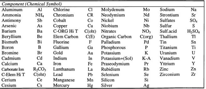
Seinfield and Pandis (1998) give a definition of PM as "any substance, except pure water, that exists as a liquid or solid in the atmosphere under normal conditions and is of microscopic or submicroscopic size but is larger than molecular dimensions". Particulate matter along with carbon monoxide (CO), sulfur dioxide (SO 2), nitrogen oxides (NOx), volatile organic compounds (VOC) and ammonia (NH3), are major contributors to urban and regional pollution. PM is by far the most complex component of atmospheric pollutants: it varies widely in term of composition, size, lifetime in the atmosphere and type of origin. PM can indeed be of primary origin (meaning emitted by a local source: terrestrial and/or anthropogenic) or of secondary origin (formed through chemical reaction within the atmosphere, involving primary origin gaseous pollutants). While secondary origin aerosol properties are highly uncertain, primary sources are generally thought to be the dominant contribution to observed concentrations. Dusek (2000) gives an average of 80%. Table 2 gives an idea of the various components of particulate matter.

Table 2: A non-Exhaustive List of Particulate Matter Components

Component (Chemical Symbol)

Aluminum Al Chlorine Cl Molydenum Mo Sodium Na

Ammonia NH4 Chromium CR Neodymium Nd Strontium Sr

Antimony Sb Cobalt Co Nickel Ni Sulfates SO4

Arsenic As Copper Cu Niobium Nb Sulfur S

Barium Ba C-ORG Hi T C(oht) Nitrates NO3 Sulf.acid H2SO4

Beryllium Be Elem Carbon C(E) Organic Carbon C(org) Thallium TI

Bismuth Bi Fluorine F Palladium Pd Tin Sn

Boron B Gallium Ga Phosphorous P Titanium Ti

Bromine Br Gold Au Potassium K Uranium U

Cadmium Cd Indium In Potassium+(Sol) K-A Vanadium V

Calcium Ca Iron Fe Praseodymium Pr Yttrium Y

Carbonate Ion R2CO3 Lanthanum La Rubidium Rb Zinc Zn

C-Elem Hi T C(eht) Lead Pb Selenium Se Zirconium Zr

Cerium Ce Manganese Mn Silicon Si

Cesium Cs Mercury Hg Silver Ag

All those components can be divided into 6 different groups as shown in the table 3.

It is rather risky to give a estimate of the share of each PM component because it varies widely across regions, times of the year and times of the day, but measurement done by

EPA and other groups (EPA, 2001) highlights the fact that all 6 components are

significantly present in PM2.5 and have comparable shares (i.e. same order of magnitude). PM2.5 refers here to the particulates the size of which is less than 2.5ptm. PM10 is another frequently used term referring to particulates less than 10 im. These particular classes designations arise from particular pollution control policies, recognizing the need to focus on small particulates. Recent regulating efforts have focused particularly on PM2.5.

Table 3: A Possible PM Classification

PM Group Origin Main anthropogenic Source Main PM size Sulfates Mainly secondary SO2 emitted from fossil fuel e PM 2.5

(from SO2) combustion

Nitrates Mainly secondary NO, from fossil fuel combustion e PM 2.5 (from NO,) and vehicle exhaust

Black Carbon Primary Vehicle exhaust, wood burning, e PM 2.5 prescribed burning

Organic Carbon Both Secondary and Vehicle exhaust, wood burning e PM 2.5 Primary

Trace Metals Mainly Primary Fossil fuel combustion, smelting e PM 2.5

Minerals Mainly Primary Dust, agriculture e PM coarse'

: PM the size of which is greater than 2.5 pm and less than 10pgm

Source: EPA (2001)

Space and Time Differences

Two particular aspects that distinguish climate change impacts and urban pollution are time and distances. Indeed, today's pollution is induced by today's emissions whereas today's greenhouse effect is induced by today's emissions but also emissions that occurred across the past century. In the same way, the global climate change effect that could occur in a hundred years from now will be caused by future 2100' emissions, but also by today's emissions. Indeed, in the greenhouse effect, it is the fact that gases (e.g

C0

impacts. Carbon dioxide (CC2, the most important greenhouse gas) has for example an

average lifetime of over a century. On the contrary, PM2.5 (particulates the size of which does not exceed 2.5pjm, like BC for example) usually have lifetimes in the atmosphere that vary from days to weeks (Panyacosit, 2000). In addition, climate effects need to be

considered as a global issue -since atmospheric gases travel all across the globe- whereas other pollutants have long been considered as a local phenomenon. The sources of pollution are usually very close from the locus of its impacts. Emissions of PM2.5 typically do not travel distances bigger than a couple of thousands kilometers (Panyacosit, 2000). This conventional wisdom has changed somewhat with new work. Recent studies (e.g. Wang, 2002) demonstrated that under certain conditions, black carbon can travel larger distances than previously thought, with significant intercontinental transport.

Health Impacts and other Ancillary Effects

Describing and understanding health impacts associated with urban pollutants, and especially PM, is a broad subject, so I will limit myself to some facts that can be of importance in understanding the goals of this thesis.

Health impacts associated with PM occur of course close to very large urban agglomerations. External factors such as climate (e.g. pollutant transport) or topography (e.g. cities close to a body of water, cities surrounded by mountains, etc...) may increase significantly those effects.

PM is considered as dangerous mainly because it can penetrate the respiratory system. As shown in table 4, the smaller the particle, the further its penetration in the respiratory system.

Table 4: PM Penetration in the Human Respiratory System

Particle size (range) Penetration of particles

11 Im and up particles do not penetrate

7-11 grm particles penetrate nasal passages

4.7-7 gm particles penetrate pharynx

3.3 - 4.7pjm particles penetrate trachea and primary bronchi 2.1 -3.3pjm particles penetrate secondary bronchi

1.1 - 2.2 m particles penetrate terminal bronchi 0.65 - 1. Im particles penetrate bronchioli 0.43 - 0.65pm particles penetrate alveoli Source: adapted from Panyacosit (2000)

The role of size of particles has been thus clearly identified: it drives the penetration of the particles. The role of the composition of the particulates is less clear: some patterns seem to appear (e.g. (Koch, 2000) and (EPA, 2000)), but no conclusion about the role of composition of PM can be drawn. It is indeed all the harder to separate the composition

effect since most of -if not all- subjects have been exposed to all the components of PM, and not only to one of them.

According to the ExternE study (European Commission, 1998), that summarizes recent studies on air pollution impact and correlation between pollution level and health impacts, the effects of PM on human health can vary from chronic bronchitis, chronic coughs, congestive heart failure, lower respiratory symptoms (wheeze) or heart diseases.

Black carbon (and aerosols generally) also contributes to a reduction in atmospheric visibility (Streets et al., 2001, Penner and Novakov, 1996).

3.

BC

I used the EPPA model to study the interactions of climate policy and air

pollution. The EPPA model was designed to study climate policy. For my purpose, I added to the model a capability to study policy directed towards BC and PM. In this chapter, I briefly review the EPPA model before describing in details the additional components I added to it.

3.1 Introduction to the EPPA Model

The Emission Prediction and Policy Analysis (EPPA) model is a recursive dynamic multi-sector multi-region world economy general equilibrium model developed

by the MIT Joint Program on Science and Policy of Global Change (Yang et al., 1996,

Babiker et al., 2001). The model was originally based on the General Equilibrium Environmental (GREEN) model (Burgniaux et al., 1992). Contrary to the GREEN model, the EPPA model was built using the MPSGE (Mathematical Programming Subsystem for General Equilibrium, (Rutherford, 1995), (Rutherford, 1999)) within the mathematical modelling language GAMS (Generalized Algebraic Modelling System, Brooke, Kendrick and Meeraus, 1996), languages with specific applicability to developing and solving Computable General Equilibrium (CGE) models.

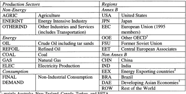
The EPPA model was designed to achieve the dual goal of forecasting greenhouse gases emissions and assessing control policy options. It is calibrated on a 1995 comprehensive economic-energy dataset (GTAP-E8_{, Hertel, 1997), that contains a} complete and detailed representation of energy systems in physical terms as well as regional productions and trade flows in economic values. GTAP data was aggregated in the model into 12 regions and 8 sectors (see figure 2)9. Production sectors use labor,

capital, energy resources and inputs of material from other production sectors. Each region's representative consumer tries to maximize its utility while each production sector within each region tries to maximize its profit. Once calibrated for the initial year

8 For more information on that, see Babiker et al (2001)

9 The version 3.0 which most of the tests were made with is currently being updated in a more

disaggregated and more geographically oriented version. However, for the purpose of simplicity, only version 3.0 (from 1999) is presented in this thesis

that is set in 1995, the model is solved for a sequence of static equilibria through 2100 in five-year time steps.

Figure 2: Regions and Sectors in EPPA

Production Sectors Regions

Non-Energy Annex B

AGRIC Agriculture USA United States ENERINT Energy Intensive Industry JPN Japan

OTHERIND Other Industries and Services EEC European Union (1995

1 (includes Transportation) members)

Energy OOE Other OECD'

OIL Crude Oil including tar sands FSU Former Soviet Union REFOIL Refined Oil EET Central European Associates

COAL Coal Non Annex B

GAS Natural Gas CHN China

ELEC Electricity Production IND India

Consumption EEX Energy Exporting countries2

FINAL Non-Industrial Consumption BRA Brazil

DEMAND DAE Developing Asian Economies3

ROW Rest of the World

1: mainly Australia, New Zealand, Canada, Turkey, and EFTA

2: OPEC and other gas-exporting, oil-exporting and coal-exporting countries 3: South Korea, Philippines, Thailand and Singapore

3.2 Modeling BC Emissions in the EPPA Model

The EPPA model aims at tracking CO2 emissions, but as well other greenhouse gases

emissions (N20, CH4 and the High GWP gases) and urban pollutants (SOx, NO,

NMVOC 0, NH3, BC, OC"). The specific model structure and data needed to model each

of these are discussed elsewhere (see Babiker et al., 2001). My focus here is on BC and

OC. The first step is to derive an inventory of BC that can be allocated to EPPA sectors. A significant portion of emissions from BC is linked to fuel-burning and thus tightly

linked in the model to fuel-consumption. Figure 3 gives a detailed relationship between actual emissions and the sectors in EPPA with which they are linked.

Emissions from black and organic carbon were derived from various sources. The previous version of the model utilized emission coefficients for fuel use derived from Cooke et al. (1999) and emissions estimates for biomass burning from Liousse et al.

(1996). I revised these inventory estimates based on more recent data and extended the 10 Non-Methane Volatile Organic Coumpound

inventories to particulate matter and black carbon. The RAINS (Regional Air Pollution Information and Simulation) model (HASA, 2003) is one important source of detailed (sector-fuel-technology) inventories of particulate matter (PM10 and PM 2.5) for European countries (including Eastern Europe and Former Soviet Union).

Streets (2001) develops an inventory of black carbon for China, using the RAINS framework. The U.S. Environmental Protection Agency (EPA) gives as well estimates for the USA for PM10 and PM2.5 (EPA, 2001). With these estimates, along with GTAP data on fuel, improved emission inventories for fuel-burning were derived for regions not covered by these data. Specifically, once detailed inventories for black carbon were derived, they were used to calculate emission factors -the emissions per unit of economic activity or fuel use in the sector. I then used these new emission factors for other regions with similar economic structure.

Figure 3: BC Emissions in the EPPA Model

Emission Sources EPPA sector

Coal-Burning in Agriculture AGRIC\COAL

Refined-Oil Burning in Agriculture AGRIC\REFOIL

Savannah Burning, Agriculture Fires, Biofuel Burning, AGRIC\NO FUEL

Livestock Emission

Industrial Coal Burning ENERINT\COAL and

OTHERIND\COAL

Coal-burning for Power Generation ELEC\COAL

Refined Oil burning for Power Generation ELEC\REFOIL

Process Emission (cement, coke production, fertilizer ENERINT\NO FUEL

production, sinter prod, non-ferrous metal smelters, pulp and paper, petroleum refineries, Pig iron production)

Refined Oil use in Industrial Transport OTHERIND\REFOIL

Refined Oil use in Household Transport FD\REFOIL

Industrial Refined Oil Burning ENERINT\REFOIL and

OTHERIND\REFOIL

Domestic Coal burning FD\COAL

Domestic Refined Oil Burning FD\REFOIL

Domestic Biofuel Burning FD\NO FUEL

As described by Mayer et al. (2000), there are a variety of reasons why these factors may change over time. In general, EPPA projections of fuel consumption (driven by economic growth forecast) would lead to very high levels and would produce dramatically high emissions of urban pollutants. But those levels are unlikely because

countries are likely to control emissions. Mayer et al. (2000) use a cross-section analysis

to find a declining relationship between GDP per capita and emissions per unit of energy use (for further details, see Mayer, 2000). Such a relationship was implemented in the model to reflect an increasing desire to control emissions as income levels rise. Tables 5

and 6 give an illustration of this pattern for regions of the world where detailed data was available. This approach was useful for developing future projections of emissions of these substances but did not provide the capability of estimating the costs of controlling them.

Table 5: Emission Factors for PM2.5 for Selected Countries (kT/EJ)

Sector Fuel CHN USA EEC FSU EET

ELEC Coal 18.0 4.6 17.0 22.9 109.9

Refoil 13.8 4.0 8.2 3.7 8.5

Industrial Fuel Combustion Coal 18.0 11.0 3.0 5.0 21.4

(ENERINT, OTHERIND, AGRIC) Refoil 11.3 5.0 1.0 3.3 7.5

Industrial Transport (OTHERIND) Refoil 32.5 35.5 13.8 19.8 49.3

Household Coal 65.0 71.0 27.5 39.5 98.5

Refoil 22.5 1.5 11.1 6.5 10.8

Biofuel 240.0 833.3 196.7 460.0 460.0

Source: emissions were derived from the RAINS model for EEC, EET, FSU, from EPA for the USA and from Streets et al. (2001) for China. Fuel Consumption was derived from GTAP data (used in the EPPA model) for coal and refined-oil, and from OECD energy balances for biofuel consumption.

Note: Differences across regions may not be only due to technical efficiency of removal devices, but also to the structure of production of the region

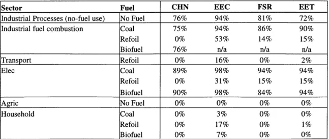
Table 6: Current PM2.5 Removal Efficiency

Sector Fuel CHN EEC FSR EET

Industrial Processes (no-fuel use) No Fuel 76% 94% 81% 72%

Industrial fuel combustion Coal 75% 94% 86% 90%

Refoil 0% 53% 14% 15%

Biofuel 76% n/a n/a n/a

Transport Refoil 0% 16% 0% 2% Elec Coal 89% 98% 94% 94% Refoil 0% 31% 15% 15% Biofuel 90% 98% 84% 94% Agric No Fuel 0% 0% 0% 0% Household Coal 0% 3% 0% 0% Refoil 0% 17% 0% 1% _Biofuel 0% 7% 0% 0%

Source: RAINS PM module for EEC, EET and FSU, available for the US

3.3 Modeling BC abatement

3.3.1 A Modeling Framework

for

In order to analyze the abatement opportunities for urban pollutants and the interactions with other policies such as climate policy, I required a relationship between abatement and marginal abatement cost that is consistent with the structure of the model.

My approach was to introduce these pollutants directly into the EPPA production

functions.

The EPPA model uses constant elasticities of substitution (CES) production functions. Each production function for each sector utilizes a wide set of inputs like capital, labor, intermediate inputs, energy inputs. The structure of the production function can be represented by the scheme shown in figure 4 and 5.

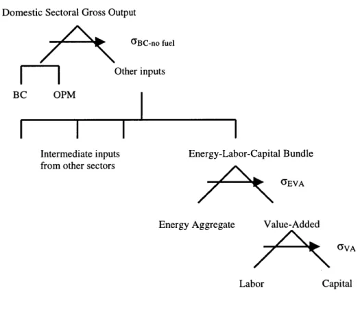
Figure 4: An Example of a Structure of Production: ENERINT and OTHERIND12 Domestic Sectoral Gross Output

I I

Intermediate inputs from other sectors

I Energy-Labor-Capital Bundle 7EVA Energy Aggregate Labor Value-Added 7VA Capital

See Babiker et al. (2001) for more details for other production sectors

Figure 5: The Energy Aggregate Nest

Energy Input

7ENOE

Elec Non-Elec

/f\X

Coal Gas Refoil

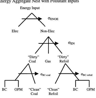
In these two structures the use of perpendicular bundles indicates a Leontieff relationship, that is to say that the elasticity of substitution between the inputs is equal to zero: the inputs are not substitutable. The non-perpendicular bundles indicate that the relationship between the inputs exhibits a constant elasticity of substitution between the inputs, and the elasticity of substitution is equal to the symbol pointed to by the arrow.

Once the framework of the production function is set, we need to insert a relationship between the production function and emissions as well as abatement opportunities. One typically thinks of emissions as an output of the production sector, the emissions being the result (indeed an externality) of the production process. However, one can consider pollutants as inputs into production (Babiker et al., 2001). Capital investments in devices that lead to a decrease in emissions factors of a pollutant can be modeled as well by the elasticity of substitution between the pollutants and the other input (Hyman, 2001).

As explained in section 2.2, we can relate most of the emissions of black carbon and other particulate matter to fuel consumption. One can thus create new bundles in the energy aggregate bundle where the pollutant input can be substituted with the fuel with a given elasticity of substitution. For the emissions that are not related to fuel consumption (e.g. biomass burning or process emissions), the same methodology developed by Hyman (2001) can be applied, that is to say create a nest at the top of the structure of the production function. In the same way, the pollutant input can be substituted by the other inputs with a given elasticity of substitution.

Finally, we need to deal with the fact that black carbon is emitted with a bulk of other pollutants in fixed proportions within the same sector. Each of the abatement technology mainly relies on filtering particulates with a certain diameter (see section 2.3) and as a consequence, those pollutants are abated in fixed proportions. If we want to introduce this pattern in the production function, we need thus to replace the single "pollutant input" by a Leontieff composite.

Figure 6 exhibits the structure of a production function where the emissions are not

linked to fuel-use whereas figure 7 shows how the implementation is achieved when the emission are linked to fuel-use13

Figure 6: A Structure of Production with a Pollutant Input at the Top (not linked with fuel-consumption), the Example of ENERINT or OTHERIND14

Domestic Sectoral Gross Output

CBC-no fuel

BC OPM

Other inputs

Intermediate inputs from other sectors

I

Energy-Labor-Capital Bundle

7EVA

Energy Aggregate Value-Added

7

Labor Capital

13 Note: biofuel-related emissions are not considered as fuel-use in this thesis because the EPPA model

does not take into account "biofuel" inputs such as wood or wastes

1 In the structure, BC stands for black carbon and OPM for other particulate matter

I

Figure 7: The Energy Aggregate Nest with Pollutant Inputs Energy Input

/YENOE

Coal Gas Refoil

GBC-coal OBC-refoil

BC OPM "Clean" "Clean" BC OPM Coal Refoil

Once we have the modeling structure of urban pollutants abatement, we need to

find an estimate of the elasticities of substitution between the pollutant and the other input. For that purpose, I will first derive a relationship between this elasticity of substitution and the marginal abatement curve for the pollutant. This is the goal of next section.

3.3.2 Derivation of the Elasticity of Substitution for Urban Pollutants

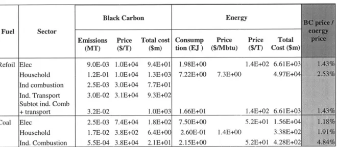
Engineering data (bottom-up analysis) can help us designing marginal abatement curves for the pollutants (in this case particulate matter, and as a consequence black carbon) by country, by sector and by type of fuel, which means that we can construct a curve with abatement in abscissa and marginal abatement cost in ordinate. However, we need to transform this data into a process where other inputs may be substituted by the pollutant5. We want thus to derive a demand function for the pollutant.

The demand function for the pollutant is simply the reverse of the abatement curve. It slopes downward as the price of the pollutant increases. The demand function can be derived from the standard production functions in EPPA.

15 This assertion of substitution with other inputs may seem peculiar, but I previously explained that the pollutants were to be treated as inputs to production in this model

As shown in figure 7, the "dirty" energy input can be obtained with two inputs: the pollutant and the "clean" energy input. In the following, we will assume that the industrial output - or the intermediate output - is produced with a pollutant input and another aggregate input.

The EPPA model utilizes constant elasticity of substitution (CES) function, which exists under a specific form. We can write the demand function and the unit production cost as follow:

Q _{= A aQI I + (I1- a)Q2a (0)}

C=qP +q₂ P2

Where

Q

C is the unit cost function

Q, is the quantity of the pollutant input Q2 is the quantity of the aggregate other input

P1 is the unit price of the pollutant input P2 is the unit price of the aggregate input

a and (1- a) are the shares of

Q

A is a scale parameter

q1 and q2 are the factor uses per unit of output

c is the elasticity of substitution between the two inputs The marginal products of Qi and Q2 are given by:

MP - -aA 6 Q"QC DQJ

2 - (l-a)A a QaQ2

MP Q22

To derive the unit cost function, we want to minimize the cost function under the constraint Q=1. We consequently have the two following first-order conditions:

-1

MP= a (q,₁

MP₂ 1-a q2

l=A aq1v +(-a)q2j (2)

P,= C.MR

P2 =C.MP2

Equation (1) thus becomes:

-1

MP _- a q_, P,

- -(i

MP₂ 1-a q2) P2

Some basic computations lead then to:

C 1= aI p-T+(1-a)P1-0)I

A

In the long run perfectly competitive equilibrium, the unit production cost equals the unit price of the output (further named Po). Thus we can restate the previous equality

PO =C = a"Pl-" + (1- af P2

A

Next, the unit demand function (i.e. the quantity of pollutant demanded to produce one unit of output) can be obtained by deriving the unit cost function (see (0)) with respect to

P1.

q, = ACa j] (3)

IP AI P, P,

As previously mentioned, a is the elasticity of substitution between the pollutant (considered as an input) and the other aggregate input.

Thus, the elasticity of substitution between the pollutant and the other aggregate input can be simply derived once we have a curve with the abatement realized in abscissa and the marginal abatement price in ordinate (see next section). Under the assumption that Po is held constant, expression (3) can indeed be restated as:

Pi

Which can be written as well as:

P, = P',(I-AP

Where P1 stands for the initial abatement price, that is to say the unit price associated with no abatement (A=0). Our curve is here completely defined by o and Pi'.

Finally, one can point out that the marginal abatement costs that I use are end-of-pipe solutions rather that reductions in the output, so we assume that there are no output