Brightest group galaxies – II: the relative contribution of BGGs to the total baryon content of groups at z < 1.3

HAL Id: hal-02110477

https://hal.archives-ouvertes.fr/hal-02110477

Submitted on 25 Apr 2019

HAL is a multi-disciplinary open access

archive for the deposit and dissemination of

sci-entific research documents, whether they are

pub-lished or not. The documents may come from

teaching and research institutions in France or

abroad, or from public or private research centers.

L’archive ouverte pluridisciplinaire HAL, est

destinée au dépôt et à la diffusion de documents

scientifiques de niveau recherche, publiés ou non,

émanant des établissements d’enseignement et de

recherche français ou étrangers, des laboratoires

publics ou privés.

Brightest group galaxies – II: the relative contribution

of BGGs to the total baryon content of groups at z 

Ghassem Gozaliasl, Alexis Finoguenov, Habib G. Khosroshahi, Bruno M. B.

Henriques, Masayuki Tanaka, Olivier Ilbert, Stijn Wuyts, Henry J.

Mccracken, Francesco Montanari

To cite this version:

Ghassem Gozaliasl, Alexis Finoguenov, Habib G. Khosroshahi, Bruno M. B. Henriques, Masayuki

Tanaka, et al.. Brightest group galaxies – II: the relative contribution of BGGs to the total baryon

content of groups at z 

Brightest group galaxies-II: the relative contribution of

BGGs to the total baryon content of groups at z <

1.3

Ghassem Gozaliasl,

, Alexis Finoguenov

, Habib G. Khosroshahi

,

Bruno M. B. Henriques

, Masayuki Tanaka

, Olivier Ilbert

, Stijn Wuyts

,

Henry J. McCracken

, and Francesco Montanari

1_{Finnish Centre for Astronomy with ESO (FINCA), University of Turku} Väisäläntie 20, FI-21500 PIIKKIÖ,Finland

2_{Department of Physics, University of Helsinki, P. O. Box 64, FI-00014, Helsinki, Finland} 3_{Helsinki Institute of Physics, P.O. Box 64, FI-00014 University of Helsinki, Finland}

4_{Max Planck-Institute for Extraterrestrial Physics, P.O. Box 1312, Giessenbachstr. 1., D-85741 Garching, Germany} 5_{School of Astronomy, Institute for Research in Fundamental Sciences (IPM), Tehran, Iran}

6_{Institute for Astronomy, ETH Zurich, CH-8093 Zurich, Switzerland} 7 _{National Astronomical Observatory of Japan, 2-21-1 Osawa, Mitaka,} Tokyo 181-8588, Japan

8 _{Aix Marseille Université, CNRS, Laboratoire ď Astrophysique de Marseille, UMR 7326, F-13388 Marseille, France} 9 _{Department of Physics, University of Bath, Claverton Down, Bath, BA2 7AY, UK}

10_{CNRS, UMR 7095 & UPMC, Institut ďAstrophysique de Paris, 98bis boulevard Arago, 75014 Paris, France}

5 October 2018

ABSTRACT

We performed a detailed study of the evolution of the star formation rate (SFR) and stellar mass of the brightest group galaxies (BGGs) and their relative contribution to the total baryon budget within R200 (fb,200BGG). The sample comprises 407 BGGs

selected from X-ray groups (M200 = 1012.8− 1014 M) out to z ∼ 1.3 identified in

the COSMOS, XMM-LSS, AEGIS fields. We find that BGGs constitute two distinct populations of quiescent and star-forming galaxies and their mean SFR is ∼ 2 dex higher than the median SFR at z < 1.3. Both the mean and the median SFRs decline with time by > 2 dex. The mean (median) of stellar mass has grown by 0.3 dex since z = 1.3 to the present day. We show that up to ∼ 45% of the stellar mass growth in a star-forming BGG can be due to its star-formation activity. With respect to fBGG

b,200, we

find it to increase with decreasing redshift by ∼ 0.35 dex while decreasing with halo mass in a redshift dependent manner. We show that the slope of the relation between fBGG

b,200 and halo mass increases negatively with decreasing redshift. This trend is driven

by an insufficient star-formation in BGGs, compared to the halo growth rate. We separately show the BGGs with the 20% highest f_b,200BGGare generally non-star-forming galaxies and grow in mass by processes not related to star formation (e.g., dry mergers and tidal striping). We present the M?− Mhand M?/Mh− Mhrelations and compare

them with semi-analytic model predictions and a number of results from the literature. We quantify the intrinsic scatter in stellar mass of BGGs at fixed halo mass (σlogM?)

and find that σlogM? increases from 0.3 dex at z ∼ 0.2 to 0.5 dex at z ∼ 1.0 due to

the bimodal distribution of stellar mass.

Key words: galaxies: clusters: general–galaxies: groups: general–galaxies: evolution– galaxies: statistics–X-rays: galaxies: clusters–galaxies: stellar content

? _{E-mail: ghassem.gozaliasl@utu.fi}

1 INTRODUCTION

The baryon content of the universe and its partitioning be-tween different components, e.g., hot/cold gas and stars, is 0000 RAS

one of the most important observations in cosmology. Clus-ters of galaxies are thought to have baryon fractions that approach the cosmic mean, with most of the baryons in the form of x-ray emitting hot gas and stars, and are par-ticularly important in this context (White & Frenk 1991). This has been confirmed by previous studies which found that, after including baryons in stars, the baryon content in the most massive clusters closely matches that measured from observations of the CMB (White et al. 1993; David et al. 1995; Vikhlinin et al. 2006; Allen et al. 2008; Dunkley et al. 2009; Simionescu et al. 2011; Bulbul et al. 2016). These features make clusters important tools to probe cosmolog-ical parameters and cosmic evolution. Several gravitational (e.g., mergers, tidal stripping) and non-gravitational (e.g., outflows from the active galactic nuclei (AGN), supernovae explosions) processes act on cluster components and play a major role in driving cluster galaxy evolution (Evrard 1997; Mohr et al. 1999; Roussel et al. 2000; Lin et al. 2003; Allen et al. 2004; McCarthy et al. 2007; Allen et al. 2008; Et-tori et al. 2009; Giodini et al. 2009; McGaugh et al. 2009; Andreon 2010; Allen et al. 2011; Simionescu et al. 2011; Dvorkin & Rephaeli 2015). These processes could account for the deviations reported between the universal baryon fraction and that of low mass clusters. The baryon frac-tion in low mass clusters or galaxy groups with halo masses Mh< 1014Mis generally smaller than the baryon fraction in massive galaxy clusters (Mathews et al 2005, Sanderson et al 2013), possibly due to AGN feedback (McCarthy et al. 2010; McCarthy et al. 2011). Admittedly, observations sug-gest that some galaxy groups with a large X-ray to opti-cal luminosity ratio (LX/Lopt) such as fossil galaxy groups (Khosroshahi et al. 2007) represent systems with a baryon fraction close to the cosmic mean value, fb= 0.16 (Mathews et al. 2005).

While studies of the cluster/group baryon fractions have been mostly focused on the estimate of the baryons con-tained in their galaxies and the hot intracluster/intragroup gas, understanding the relative contribution of the satel-lite galaxies and the brightest cluster/group galaxies (BCGs/BGGs) is highly important for precise modelling of galaxy formation especially in low-mass haloes. Giodini et al. (2009) have shown that the stellar mass fraction con-tained in 91 galaxy groups/clusters at 0.1 < z < 1.0 se-lected from the COSMOS survey scales with total mass as M₅₀₀−0.37±0.04 (M500 corresponds to the halo mass at the ra-dius at which the over-density is 500 times the mean den-sity) and is independent of redshift. Gonzalez et al. (2013) have also found that the fraction of the baryons residing in stars and hot-gas are strong functions of the total mass and scale as fstar ∝ M500−0.45±0.04 and fgas ∝ M5000.26±0.03, indicating that the baryons contained in stars become im-portant in low mass haloes. Determining the contribution of stars to the total baryon fraction in groups, as opposed to massive clusters, is also important because baryonic effects (e.g., radio feedback) are more significant in groups (e.g., Giodini et al. 2012). The primary goal of the present study is to quantify the contribution of central galaxies to the total baryonic mass of hosting groups.

In order to separate the role of different physical mech-anisms in galaxy evolution, a number of studies have con-strained stellar-to-halo mass (SHM) relations and ratios as a function of time using the abundance matching technique

(e.g. Behroozi et al. 2010a; Moster et al. 2010; Behroozi et al. 2010b), the conditional luminosity function technique pro-posed by Yang et al. (2003), the halo occupation distribution (HOD) formalism (e.g. Berlind & Weinberg 2002; Kravtsov et al. 2004; Moster et al. 2010), and by combining the HOD, N-body simulations, galaxy clustering, and galaxy-galaxy lensing techniques (e.g., Leauthaud et al. 2012; Coupon et al. 2015). Distinguishing the properties of central galaxies from those of satellite galaxies in studies based only on the dis-tribution of luminosity or stellar mass is challenging (e.g., George et al. 2011). By combining several observables and techniques (e.g. HOD, galaxy-galaxy lensing, galaxy cluster-ing) one can probe a global SHM relation for central galaxies and satellite galaxies (e.g., Leauthaud et al. 2012; Coupon et al. 2015). Coupon et al. (2015), for example, used multi-wavelength data of ∼ 60000 galaxies with spectroscopic red-shifts in the CFHTLenS/VIPERS field to constrain the rela-tionship between central/satellite mass and halo mass, char-acterising the contributions from central and satellite galax-ies in the SHM relation. In this paper, we directly identify the BGGs using their precise redshifts and estimate stel-lar masses using the broad band Spectral Energy Distribu-tion (SED) fitting technique (Ilbert et al. 2010a) as used by Coupon et al. (2015). We utilise the advantages of the X-ray selection of galaxy groups and a wealth of multi-wavelength, high signal-to-noise ratio observations such as the UltraV-ISTA survey in the COSMOS field (Laigle et al. 2016) to investigate the SHM relation for the central galaxies over 9 billion years. We aim to quantify the intrinsic (lognormal) scatter in stellar mass at fixed redshift in observations and compare them to the recently implemented semi-analytic model (SAM) by Henriques et al. (2015).

This paper is the second in a series of three studying the evolution of the properties of BGGs. We use a sample of 407 X-ray galaxy groups with halo masses ranging from ∼ 1012.8 to 1014M at 0.04 < z < 1.3 selected from the XMM-LSS (Gozaliasl et al. 2014), COSMOS (Finoguenov et al. 2007; George et al. 2011) and AEGIS (Erfanianfar et al. 2013) fields.

In the first paper in this series (Gozaliasl et al. 2016), we presented our data and the sample selection criteria. We studied the distribution of stellar mass (M?) and (specific) star-formation rate (SFR) of the BGGs and found that the stellar mass distribution of the BGGs evolves towards a nor-mal distribution with decreasing redshift. We also showed that the average M?of BGGs grows by a factor of ∼ 2 from z = 1.3 to the present day. This M? growth slows down at z < 0.5 in contrast to the SAM predictions. We also revealed that BGGs are not completely quenched systems, and about 20 ± 3% of them with stellar mass of ∼ 1010.5M continue star-formation with rates up to SF R ∼ 200 Myr−1.

In this paper, we measure the total baryon content of galaxy groups and compute the ratio of the stellar mass of BGGs to the total baryonic mass of haloes within R200 as fBGG

b,200 and investigate whether this ratio changes as a function of redshift and halo mass. We showed that the mean value of the SFR of BGGs is considerably higher than the median value of SFR and the mean value is influenced by the very high SFRs. Thus, we decided to investigate the evolution of both mean and median values of SFR, M?, and fb,200BGG, individually. Similarly to the first paper of this series, we use observations here to probe the predictions by four 0000 RAS, MNRAS 000, 000–000

SAMs based on the Millennium simulation as presented in Bower et al. (2006, hereafter B06), De Lucia & Blaizot (2007, hereafter DLB07), Guo et al. (2011, hereafter G11), and Henriques et al. (2015, hereafter H15).

This paper is organised as follows: we briefly describe our sample in section 2; Section 3 presents the relation be-tween fBGG

b,200 and Mh (Mhcorresponds to M200c or M200m , where the internal density of haloes is 200 times the crit-ical or mean density of the universe). We investigate the smoothed distribution of fb,200BGG in different redshift bins. We also examine the redshift evolution of the mean (me-dian) value of SF R, M?and fb,200BGG. Section 3 also presents the SHM relation and ratio and assigns a lognormal scatter in the stellar mass of BGGs at fixed halo mass. We compare our findings with a number of results from the literature. Section 4 summaries the results and conclusions.

Unless stated otherwise, we adopt a cosmological model, with (ΩΛ, ΩM, h) = (0.70, 0.3, 0.71), where the Hubble con-stant is parametrised as 100 h km s−1 Mpc−1 and quote uncertainties as being on the 68% confidence level.

2 DATA OF BGGS

2.1 Sample definition and BGG selection

We use galaxy group catalogues, with Mh ∼ 5 × 1012 to 1014.5_M

at 0.04 < z < 1.9, which have been selected from the COSMOS (Finoguenov et al. 2007; George et al. 2011), XMM–LSS (Gozaliasl et al. 2014), and AEGIS (Erfanianfar et al. 2013) fields. To ensure the high quality of the pho-tometric redshift of groups, we constrain our study to the redshift range of 0.04 < z < 1.3 and study groups with halo mass ranging from Mh ' 7.25 × 1012 to 1.04 × 1014(M). As in Fig. 1 of paper I (Gozaliasl et al. 2016), we define five subsamples of galaxy groups considering their halo mass-redshift plane as follows:

(S-I) 0.04 < z < 0.40 & 12.85 < log(M200

M ) 6 13.50

(S-II) 0.10 < z6 0.4 & 13.50 < log(M200

M ) 6 14.02

(S-III) 0.4 < z6 0.70 & 13.50 < log(M200

M ) 6 14.02

(S-IV) 0.70 < z6 1.0 & 13.50 < log(M200

M ) 6 14.02

(S-V) 1.0 < z6 1.3 & 13.50 < log(M200

M ) 6 14.02

Four subsamples (S-II to S-V) cover a similar narrow halo mass range, which allows us to compare the stellar properties of BGGs within haloes of the same masses at dif-ferent redshifts. The subsample of S-I has a similar redshift range to that of S-II but with a different halo mass range, which enables us to inspect the impact of halo mass on the properties of BGGs at z < 0.4.

The full details of the sample selection, stellar mass and halo mass measurements have been presented in Gozaliasl et al. (2016) and Gozaliasl et al. (2014). We estimate the halo mass using the Lx− Mhrelation as presented in Leauthaud et al. (2010). We also assume a 0.08 dex extra error in the halo mass estimate in our analysis, which corresponds to a log-normal scatter of the Lx− Mhrelation (Allevato et al. 2012). Table 1 presents the mean stellar mass and halo mass with corresponding statistical and systematic errors for S-I to S-V. The systematic error corresponds to uncertanities in the stellar and halo mass measurements. We note that these systematic errors are taken from the galaxy and group

0.0 0.2 0.4 0.6 0.8 1.0 1.2

Redshift [z]

log

(M

/M

yr

)

13.8 11.9 10.4 9.1

Cosmic time [Gyr]

0.0

0.2

0.4

0.6

0.8

1.0

1.2

Redshift [z]

12.5

13.0

13.5

14.0

14.5

15.0

log

(M

/M

)

13.8 11.9 10.4 9.1 8.1 7.2 6.5 5.8 5.3 4.8

Cosmic time [Gyr]

COSMOS+XMM-LSS+AEGIS

Figure 1. (Upper panel) Mean mass accretion rate of dark mat-ter on to haloes ( ˙Mh) as a function of cosmic time and red-shift from z = 1.3 to z = 0 in Millennium simulations I & II (following equation 2 in Fakhouri et al. 2010). The solid lines show trends for a set of haloes of given masses, Mh = 1012.6 _M

, 1013M, 1013.4M, 1013.8M, 1014.2M. (Lower panel) The halo mass of X-ray galaxy groups selected from COS-MOS, AEGIS, and XMM-LSS fields as a function of cosmic time (z) (filled and open circles). Solid lines illustrate the redshift evo-lution of Mhfor a set of typical haloes with a given initial halo mass (as mentioned in the upper panel) from z = 1.3 to the present day. In order to investigate the impact of the halo mass growth on the evolution of stellar properties of galaxies such as stellar mass growth, we define a new sample of galaxy groups (open circles) which lie in the highlighted area (S-IHMA).

catalogues by Finoguenov et al. (2007); Wuyts et al. (2011); Erfanianfar et al. (2013); Gozaliasl et al. (2014); Laigle et al. (2016).

According to the cold dark matter (CDM) hierarchi-cal structure formation paradigm, dark matter haloes grow by accretion of matter and merging with other (sub)haloes (Frenk et al. 1988). It is well-known that many of the ob-served galaxy properties correlate with the environment such as the known positive correlation between the stel-lar mass of the BCGs/BGGs and the halo mass of their host dark matter haloes (Gozaliasl et al. 2016). The slope of this correlation is less than unity, implying that the clus-ter growth is fasclus-ter than the BCG growth at the same 0000 RAS, MNRAS 000, 000–000

time. As a result, it is important that the effect of halo growth is taken into account, when galaxy growth is de-termined. To do this, we use the results presented by Fakhouri et al. (2010) who construct merger trees of dark matter haloes and estimate their merger rates and mass growth rates using the joint data set of the Millennium I and Millennium-II simulations. We use equation 2 by Fakhouri et al. (2010) and determine the mean halo mass growth rates for some typical haloes of given masses (Mh= 1012.6 _M

, 1013 M, 1013.4 M, 1013.8 M, 1014.2 M) at z = 1.3. As shown in Fig. 1, the mean mass growth rate slowly decreases with cosmic time for all halo masses. Con-sidering these mass accretion rates, we determine whether Mh of these set of haloes grow with cosmic time (z) from z = 1.3 to the present day (solid lines in the lower panel of Fig. 1).

Following the method used by Groenewald (2016), we construct an evolutionary sequence of galaxy groups at z < 1.3, then select a new sample of galaxy groups such that their masses lie in the narrow highlighted cyan area and between two halo mass limits (green and red lines), which represent the Mh growth for two dark matter haloes with initial masses of 1013.4and 1013.8Mat z = 1.3, respectively. If a group with Mh± 1σ falls in the highlighted area, it is also included in the sample. We analyse this new sample of groups and the associated BGGs at 0.2 < z < 1.3 in §3.3 and compare the results with those for subsamples of II to S-V, where the halo mass range is the same for all subsamples and halo mass growth is not taken into account. Hereafter, we will refer to the new Sample with Including Halo Mass Assembly effect as S-IHMA.

We select most of the BGGs from groups by cross-matching their spectroscopic redshifts with the redshift of groups. BGGs with no spectroscopic observations are se-lected using their photometric redshift (Wuyts et al. 2011; McCracken et al. 2012; Ilbert et al. 2013; Laigle et al. 2016) and the colour-magnitude diagram of group members, as described in detail in Gozaliasl et al. (2014). In this paper, the physical properties of BGGs in the COSMOS field are taken from the COSMOS2015 catalogue (Laigle et al. 2016). This catalogue contains 1, 182, 103 objects with a high pho-tometric redshift precision of σ∆z/(1+zsec)= 0.007 in the 1.5 deg2UltraVISTA-DR2 region. For more detail on the photo-metric redshift calculation/precision and physical parameter measurement of galaxies, we refer the reader to Laigle et al. (2016).

The sample selection for this work relies on the detec-tion of the outskirts of X-ray galaxy groups. As such, this sample is unbiased towards the presence of the cool cores and therefore the properties of the BCGs. The difference in the completeness are minimized by selecting a relatively narrow range of halo masses for the study. As reported in Tab. 1, the differences (. 0.11 dex) among the mean halo mass of haloes for S-II to S-V lie within the total error.

2.2 Semi-analytic models

We compare our results with a number of theoretical stud-ies, namely with four semi-analytic models (SAMs): Bower et al. (2006) (B06); De Lucia & Blaizot (2007) (DLB07); Guo et al. (2011) (G11); Henriques et al. (2015) (H15). All the models are based on merger trees from the Millennium

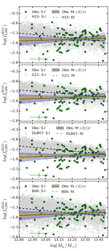
Sim-Figure 2. The relative contribution of the stellar populations of the BGGs to the total baryonic mass of hosting groups, log(fBGG

200 ), as a function of halo mass (log(Mh/M)). Each row from top to bottom compares the observational data (filled green circles) with the data taken from SAMs of H15, G11, DLB07, and B06 (open gray squares), respectively. The best-fit relation to the data in observations with associated ±1σ and ±2σ confidence intervals are shown as the solid green lines and the highlighted orange and blue regions. The best-fit relation for the SAMs are plotted as the dashed black lines. In each plot, we have shown the scale of the median of observed uncertainties on the log(Mh/M) and log(fBGG

200 ) estimates with green error bars.

Table 1. The average systematic error (SYSE) and the statistical error on the mean (SEM) of log(M?/M) and log(Mh/M) for S-I to S-V. The error values are given in dex.

Sample hlog(M?/M)i dM?(SYSE) dM?(SEM) hlog(Mh/M)i dMh(SYSE) dMh(SEM)

S-I 10.84 0.12 0.08 13.28 0.16 0.01

S-II 11.06 0.15 0.07 13.68 0.12 0.02

S-III 11.15 0.16 0.07 13.69 0.15 0.01

S-IV 11.02 0.15 0.05 13.75 0.15 0.01

S-V 10.89 0.19 0.05 13.79 0.16 0.02

ulation (Springel et al. 2005) which provides a description of the evolution of dark matter structures in a cosmological volume. While B06, DLB07 and G11 use the simulation in its original WMAP1 cosmology, H15 scales the merger trees to follow the evolution of large scale structures expressed for the more recent cosmological measurements. With respect to the treatment of baryonic physics, B06 uses the GALFORM version of the Durham model, while DLB07, G11, and H15 follow the Munich L-Galaxies model.

In Gozaliasl et al. (2014), we described some impor-tant features of the G11, DLB07, and B06 models. We thus, briefly describe the recent improvements and modifications in the H15 model here and the reader is referred to the Hen-riques et al. (2015) for further details. With respect to the previous version of L-Galaxies, in addition to the implemen-tation of a PLANCK cosmology, Henriques et al. (2015) uses the Henriques et al. (2013) model for the reincorporation of gas ejected from SN feedback. The scaling of reincorporation time with virial mass, instead of virial velocity, suppresses star-formation in low mass galaxies at earlier times and re-sults in an excellent match between theoretical and observed stellar mass functions at least since z = 3.

In addition, the H15 model assumes that ram-pressure stripping is only effective in clusters (Mvir> 1.2 × 1014M) and has a cold gas surface density threshold for star-formation that is ∼ two times smaller than in earlier models. These two modifications ensure that satellite galaxies retain more fuel for star-formation and continue to form stars for longer. This eases a long standing problem with satellite galaxies in theoretical models being quenched too quickly and provides a good match to quenching trends as a func-tion of environment (Henriques et al. 2016). Finally, H15 modified the AGN radio mode accretion rate in order to en-hance accretion at z < 0.5 with respect to earlier times and ensure that galaxies around M* grow significantly down to that redshift, but are predominantly quenched in the local universe.

3 RESULTS

3.1 The halo mass dependence of the stellar baryon fractions contained in the BGGs Galaxy clusters/groups are large enough to represent the mean matter distribution of the Universe (White et al. 1993), thus the ratio of their total baryonic mass (stars, stellar remnants, and gas; Mb) to their total mass including dark matter (Mtot) is expected to match the ratio of Ωb to Ωmfor the universe

fb= Mb Mtot = Ωb Ωm . (1)

We use cosmological parameters from the full-mission Planck satellite observations of temperature and polarisa-tion anisotropies of the cosmic microwave background ra-diation (CMB) and Baryon Acoustic Oscillations (BAO) and estimate the observed baryon fraction of the universe (Ωbh−2 = 0.02226 ± 0.00023, Ωmh−2 = 0.1415 ± 0.0019, fb = 0.1573 ± 0.0037) (Ade et al. 2015) and determine the total baryonic mass of each galaxy group within R200 as Mb,200= fbM200.

In order to quantify the contribution of the BGG stellar component to the total group baryons in observations and SAMs, we estimate the ratio of the stellar mass of BGGs to the total baryonic mass of hosting groups as follows

fb,200BGG= M?BGG Mb,200 = (Ωb Ωm )−1(M BGG ∗ M200 ), (2)

where fb,200BGG defines the fraction of the total baryon of a group within r ∼ R200 contained in stars of the BGG. In §3.1 to 3.2, we only compare our results with predictions from four SAMs (Bower et al. 2006; De Lucia & Blaizot 2007; Guo et al. 2011; Henriques et al. 2015). The halo mass of groups (Mh) in all these models correspond to M200c, we thus prefer to also use the M200c of groups in observations. However, we convert M200c to M200m in the rest of results presented in §3.4 to 3.6.

In Fig. 2 to 4 , we focus on the halo mass dependency of the fBGG

b,200. The data associated with the observed sample are shown as filled green circles while the data for the SAMs as shown with open grey squares. Panels from top to bottom compare observations with the SAM of H15, G11, DLB07, and B06, respectively. We approximate the observed and predicted data using a power law relation (e.g., Giodini et al. 2009) given by

fb,200BGG= β × ( Mh M

)α, (3)

where α and β present the power low exponent and con-stant of the fb,200BGG− Mhrelationship. We take advantage of the properties of logarithms and convert this relation into a linear relationship given by

log (fb,200BGG) = log (β) + α × log ( Mh M

), (4)

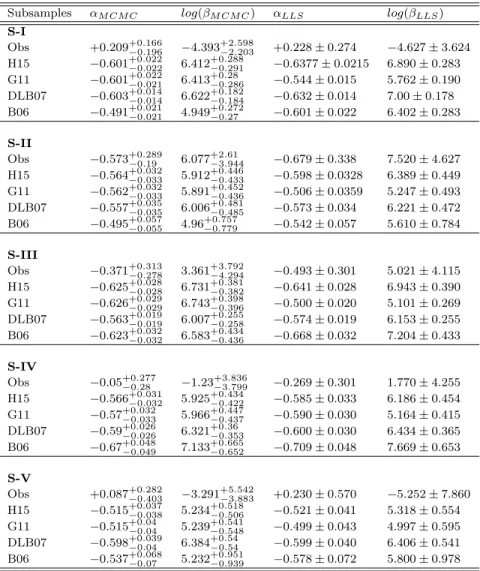
we fit this equation to data and quantify the best-fit and optimised parameters by the Linear Least Squares approach and the Markov chain Monte Carlo (MCMC) method in Tab. 2. Since the fitted parameters by two methods are compa-rable in some cases, we decide to report both parameters in this table. The first column of Tab. 2 presents the sub-sample ID. The second and third columns present αM CM C 0000 RAS, MNRAS 000, 000–000

Table 2. The parameters of the best-fit relation, log(fBGG

b,200) = α × log(M200/M) + log(β), obtained by linear least squares (LLS) and Markov chain Monte Carlo (MCMC) methods for both observations and SAMs. The first column presents the id of subsamples. The second and the third columns list the optimised parameters with 68% confidence intervals by the MCMC method. The fourth and fifth columns present the parameters with ±1σ error obtained by LLS.

Subsamples αM CM C log(βM CM C) αLLS log(βLLS) S-I Obs +0.209+0.166_−0.196 −4.393+2.598_−2.203 +0.228 ± 0.274 −4.627 ± 3.624 H15 −0.601+0.022_−0.022 6.412+0.288−0.291 −0.6377 ± 0.0215 6.890 ± 0.283 G11 −0.601+0.022 −0.021 6.413+0.28−0.286 −0.544 ± 0.015 5.762 ± 0.190 DLB07 −0.603+0.014 −0.014 6.622+0.182−0.184 −0.632 ± 0.014 7.00 ± 0.178 B06 −0.491+0.021_−0.021 4.949+0.272_−0.27 −0.601 ± 0.022 6.402 ± 0.283 S-II Obs −0.573+0.289 −0.19 6.077+2.61−3.944 −0.679 ± 0.338 7.520 ± 4.627 H15 −0.564+0.032_−0.033 5.912+0.446_−0.433 −0.598 ± 0.0328 6.389 ± 0.449 G11 −0.562+0.032_−0.033 5.891+0.452−0.436 −0.506 ± 0.0359 5.247 ± 0.493 DLB07 −0.557+0.035_−0.035 6.006+0.481−0.485 −0.573 ± 0.034 6.221 ± 0.472 B06 −0.495+0.057 −0.055 4.96+0.757−0.779 −0.542 ± 0.057 5.610 ± 0.784 S-III Obs −0.371+0.313_−0.278 3.361+3.792−4.294 −0.493 ± 0.301 5.021 ± 4.115 H15 −0.625+0.028 −0.028 6.731+0.381−0.382 −0.641 ± 0.028 6.943 ± 0.390 G11 −0.626+0.029 −0.029 6.743 +0.398 −0.396 −0.500 ± 0.020 5.101 ± 0.269 DLB07 −0.563+0.019_−0.019 6.007+0.255_−0.258 −0.574 ± 0.019 6.153 ± 0.255 B06 −0.623+0.032_−0.032 6.583+0.434−0.436 −0.668 ± 0.032 7.204 ± 0.433 S-IV Obs −0.05+0.277_−0.28 −1.23+3.836_−3.799 −0.269 ± 0.301 1.770 ± 4.255 H15 −0.566+0.031_−0.032 5.925+0.434−0.422 −0.585 ± 0.033 6.186 ± 0.454 G11 −0.57+0.032_−0.033 5.966+0.447−0.437 −0.590 ± 0.030 5.164 ± 0.415 DLB07 −0.59+0.026 −0.026 6.321+0.36−0.353 −0.600 ± 0.030 6.434 ± 0.365 B06 −0.67+0.048 −0.049 7.133 +0.665 −0.652 −0.709 ± 0.048 7.669 ± 0.653 S-V Obs +0.087+0.282−0.403 −3.291+5.542−3.883 +0.230 ± 0.570 −5.252 ± 7.860 H15 −0.515+0.037_−0.038 5.234+0.518_−0.506 −0.521 ± 0.041 5.318 ± 0.554 G11 −0.515+0.04_−0.04 5.239+0.541_−0.548 −0.499 ± 0.043 4.997 ± 0.595 DLB07 −0.598+0.039_−0.04 6.384+0.54−0.54 −0.599 ± 0.040 6.406 ± 0.541 B06 −0.537+0.068 −0.07 5.232+0.951−0.939 −0.578 ± 0.072 5.800 ± 0.978

and log (βM CM C) with corresponding 68% confidence inter-val, respectively. The 4thand 5thcolumns report αLSS and log (βLLS) with ±1σ uncertainties, respectively.

In Fig. 2 to 4, the solid green and dashed black lines il-lustrate the LLS best-fit relations in observations and SAMs, respectively. Our major findings are as follows:

(i) For S-I (Fig. 2), we find that log(fb,200BGG) shows no significant dependence on log(Mh/M), while models show that log(fb,200BGG) decreases with increasing log(Mh/M). We note that the best-fit relation to the observational data might be affected due to insufficient number of the low-mass haloes at log(Mh/M) < 13.15. Beyond this mass, observa-tions and models become consistent.

(ii) For S-II (Fig. 3, left), we find that log(fBGG b,200) de-creases as a function of increasing log(Mh/M), in a good agreement with all model predictions within ±2σ errors. Among the models, H15 and B06 are more successful in predicting the observed trend.

(iii) For S-III (Fig. 3, right), log(fBGG

b,200) also decreases as a function of increasing log(Mh/M). The models are consistent with the observed trend within ±2σ errors. It

appears that B06 underestimates log(fBGG

b,200) at a given halo mass.

(iv) For S-IV (Fig. 4, left), we find that log(fb,200BGG) de-creases slowly as a function of increasing log(Mh/M), in agreement with models within ±2σ uncertainties.

(v) For S-V (Fig. 4, right), we find that log(fBGG b,200) in-creases slowly as a function of increasing log(Mh/M), which is in contrast with most of the model predictions.

In summary, the observed log(fb,200BGG) is found to de-crease as a function of increasing log(Mh/M) a trend which is mildly redshift dependent. The models predict a similar trend but with no significant dependence on redshift.

At z < 0.4, we find that log(fb,200BGG) - log(Mh/M) rela-tion within haloes with Mh< 1013.5M show an opposite trend compared to the trend within massive haloes.

SAMs generally reproduce the observed fBGG b,200 − M200 relation of BGGs for S-II to S-V within the uncertainty, however, they fail to adequately predict this relation for S-I. 0000 RAS, MNRAS 000, 000–000

Figure 3. The relative contribution of the BGGs to the total baryonic mass of hosting groups, log(fBGG

200 ), as a function of halo mass (log(Mh/M)). Same as in Fig. 2 but for S-II (left column) and S-III (right column), respectively.

3.2 Distribution of fBGG b,200

In Fig. 5, we present the distribution of fb,200BGG (grey his-togram). To compare the observations to models, we use the Kernel Density Estimation (KDE) technique (Rosenblatt 1956) and determine the smoothed distribution of fBGG

b,200 in observations (solid black line) and the SAMs of H15 (solid magenta line), G11 (dotted red line), DLB07 ( dashed green

line), and B06 (dash-dotted blue line). The y-axes in this dis-tribution display the probability density function and they are normalised in a way that the area under the curves is unity. The lower right panel present the smoothed distribu-tion of fb,200BGGfor S-I to S-V and the full sample of BGGs in observations. The rest of panels illustrate the results in ob-servations and models for S-I to S-V, separately. Our main findings in each panel of Fig. 5 are as follows:

Figure 4. The relative contribution of the BGGs to the total baryonic mass of hosting groups, log(fBGG

200 ), as a function of halo mass (log(Mh/M)). The same as in Fig. 2 but for S-IV (left column) and S-V (right column), respectively.

(i) For S-I, the fBGG

b,200 distribution spans between ∼ 0.002 and 0.18. All SAMs overestimate the position of the cen-tre of the peak (mean value) in the observed distribution. Among them, H15 and B06 predictions are closer to the ob-servations.

(ii) For S-II, the fb,200BGGdistribution extends over 0.004 to 0.06. All the models overestimate the height of the peak.

However, H15 and B06 predict correctly the position of the centre of the observed peak.

(iii) For S-III, the fb,200BGG distribution ranges between 0.001 and 0.08. All models overestimate the height of the peak in the observed distribution. H15 and B06 underesti-mate the position of the centre of the peak. It appears that models also underestimate the observed probability distri-bution function at high fBGG

b,200.

Figure 5. Distribution of fBGG

200 in observations (solid grey histogram). The smoothed observed distribution (KDE) (solid black line) is compared to those from SAMs of G11 (dotted red line), DLB07 (dashed green line), B06 (dashed-dotted line), and H15 (solid magenta line), respectively. The lower right panel compares the observed KDE functions among S-I to S-V and that of the whole sample of 407 BGGs in observations (solid cyan distribution). The large black ticks (rugs) present the observed one-dimensional density along fBGG

200 -axis.

(iv) The fb,200BGGdistribution for S-IV spans between 0.0005 and 0.055. The height of the peak is overestimated by all the models. Among models, H15 better predicts the obser-vations.

(v) The fBGG

b,200 distribution for S-V extends from 0.0003 to 0.037. DLB07, G11, and H15 all over-predict the centre of the peak, while the B06 prediction is in a good agreement with observations.

(vi) The lower right panel of Fig. 5 compares the smoothed distribution of fb,200BGGin observations for I to S-V. We find that the position of the centre of the peak tends to move to lower values with increasing redshift. In addi-tion, we observe that the height of the peak also increases with increasing redshifts of BGGs. The significant changes in the distribution of fb,200BGG occur at z ∼ 0.7. This com-parison shows that fBGG

b,200 evolves with redshift. As a result, the fraction of BGGs that contribute strongly to the total baryon budget of hosting groups increases with decreasing redshift, suggesting that BGGs may grow considerably in stellar mass at z < 1.3.

In addition, we find that the fBGG

b,200 distribution for S-I skews more to higher values along the x-axes compared to BGGs within massive groups. This indicates that the central galaxies in the low-mass haloes contribute strongly to the total baryonic content of haloes.

3.3 Evolution of SFR, M?, and fb,200BGG of BGGs In Fig. 5, we find evidence for the redshift evolution of the fb,200BGG distribution. To understand the origin of this evolu-tion, we investigate the stellar mass, SFR, and log(fBGG

b,200) of the BGGs for S-II to S-V and S-IHMA. We described both data sets in detail in §2.1. We determine the mean and median values of log(SF R/Myr−1) (hereafter log(SF R)) , log(M?/M) (hereafter log(M?)), and log(f200BGG) for S-II to S-V. We also measured these quantities for S-IHMA within 5 redshift bins.

We note that the halo mass growth is taken into account in the sample selection for S-IHMA, while this effect is not considered in the BGG selection for S-II to S-V. The left and right columns of Fig. 6 show results for S-II to S-V and S-IHMA, respectively.

To gain further knowledge on the relative contribution of the BGG stars to the total baryon content of groups, we repeat the same computation for 20% of the BGGs with the highest f200BGG in each redshift bin for both S-II to S-V and S-IHMA, as presented in Fig. 7.

The upper, middle and bottom panels of Fig. 6 and Fig. 7 show the mean and median values of log(SF R/Myr−1) (hereafter log(SF R)) , log(M?/M) (hereafter log(M?)), and log(fBGG

200 ) versus redshift. We describe these relation-ships in §3.3.1 to §3.3.3, respectively.

3.3.1 The SFR evolution of BGGs

In Gozaliasl et al. (2016), we have shown that ∼ 25% and ∼ 60% of the BGGs lie on the main sequence of the star forming galaxies at 0.4 < z < 0.5 and 1 < z < 1.3, respec-tively. The SFRs of these galaxies can reach up to ∼ 100 × solar mass per year, in a good agreement with a similar study on 90 BCGs selected from the X-ray galaxy clusters

in the 2500-square-degree South Pole Telescope survey by McDonald et al. (2016). They have also found that the SFR of 34% of the BCGs exceeds 10Myr−1 at 0.25 < z < 1.25 and this fraction rises up to 92+6−31% at z > 1.

In this paper, we study the redshift evolution of the mean (median) log(SF R) of the BGG to find out what frac-tion of the M?and fb,200BGGgrowth at z < 1.3 could be driven by the star formation.

The upper panel in Fig. 6 illustrates mean (median) log(SF R) as a function of redshift for BGG within S-II to S-V (left) and BGG within S-IHMA (right). The filled/open black points show the data in the observations. The solid (dashed) green, red, and magenta lines indicate the mean (median) log(SF R) − z relations in the SAMs by DLB07, G11, and H15, respectively. We find that the BGG SFRs in both observations and models follow a bimodal distribution, implying that the mean SFR deviates significantly from the median SFR. In addition, this indicates that BGGs consist of two distinct populations of quiescent and star forming galaxies.

The data in observations shows a rapid evolution at z > 0.7. This causes the observed trend over 0.1 < z < 1.3 to deviate from a linear form. Thus, we use two non-linear relations such as

f (z) = α × zβ+ γ, (5)

or the quadratic polynomial

f (z) = a + b × z + c × z2, (6) to reproduce the trend in the observations. We fit both re-lation to the data and select the best one. We also note that these best-fit relations may not be valid beyond the redshift range of our BGG sample (0.1 < z < 1.3). The highlighted grey area represents ±1σ confidence intervals.

Just as in Fig.6, we measure the redshift evolution of mean (median) log(SF R) for 20% of BGGs with the highest fBGG

b,200 for S-II to S-V and S-IHMA in the upper panel of Fig. 7. Tab. 3 presents the best-fit log(SF R) − z relations.

We summarise the observed and predicted log(SF R)−z relations as follows:

(i) The mean (median) log(SF R) of BGGs for both S-II to S-V and S-IHMA decrease considerably with cosmic time by ∼ 2 dex since z = 1.3. A significant decline occurs at z > 0.7. Including the halo mass growth in sample selection has no considerable impact on the evolution of star formation in BGGs at z < 1.3.

The mean log(SF R) of 20% of BGGs with the highest fb,200BGG for both S-II to S-V and S-IHMA also decrease in time by ∼ 2 and 4 dex since z = 1.3 to the present day, respectively. It appears that accounting for the halo mass growth in sample selection causes the SFR of BGGs with the highest fb,200BGG to decline more efficiently.

The median log(SF R) of BGGs (20%) with the highest fBGG

b,200 show no significant changes with redshift within the uncertainties at 0.2 < z < 1.2. The trend for S-IHMA shows a decrease by ∼2 dex from z=1.2 to z=0.7 followed by an increase of about 1 dex at low redshifts.

(ii) All the SAMs consistently predict that mean (me-dian) log(SF R) decreases with redshift by around 0.5 − 1 dex. At z > 0.6, they underestimate the observed mean 0000 RAS, MNRAS 000, 000–000

0.2 0.4 0.6 0.8 1.0 1.2 5 4 3 2 1 0 1 2

log

(S

FR

/M

yr

1

)

BGGs (S-II to S-V)

H15

G11

DLB07

Obs

11.9

Cosmic time [Gyr]

mean value

H15

G11

DLB07

Obs

log

(M

/M

)

BGGs (S-II to S-V)

B06 (mean)

B06 (median)

M growth via mean SFR(z)

M growth via median SFR(z)

0.2 0.4 0.6 0.8 1.0 1.2

Redshift [z]

log

(f

BG

G

b,

20

0

)

BGGs (S-II to S-V)

f

growth via mean SFR(z)

f

growth via median SFR(z)

0.2 0.4 0.6 0.8 1.0 1.2 4 3 2 1 0 1 2

BGGs (S-IHMA)

11.9

Cosmic time [Gyr]

0.2 0.4 0.6 0.8 1.0 1.2 10.7 10.8 10.9 11.0 11.1 11.2 11.3 11.4 11.5

BGGs (S-IHMA)

Redshift [z]

BGGs (S-IHMA)

Figure 6. ( Upper panels) the mean (median) of log(SF R/Myr−1) as a function of redshift for S-II to S-V (left panel) and S-IHMA (right panel). The solid (dashed) black lines show the best-fit function to the mean (median) of log(SF R/Myr−1) versus redshift in observations. The mean (median) of log(SF R/Myr−1) − z relations in predictions by H15, G11, and DLB07 are shown with solid (dashed) magenta, red, and green lines, respectively. (Middle panels) same as in the upper panel but for log (M?/M ) as a function of redshift. We highlight the area between the mean and median trends in model predictions. The cyan solid (dashed) line shows the M? growths for typical BGGs through the mean (median) SFR-z relations with initial stellar masses which correspond to the mean (median) of stellar mass of BGGs for S-V. ( Lower panels) the average/median value of log(fBGG

200 ) versus redshift for S-II to S-V (left panel) and S-IHMA (right panel). Same as in the middle panel the shaded regions present the model predictions. The solid (dashed) cyan line shows the growth of log(fBGG

200 ) through star-formation for two typical BGGs with initial baryon fractions which correspond to the mean (median) value of log(fBGG

200 ) for S-V. Stars in these two typical BGGs are formed in time with mean (median) rate which we approximate in the upper panel.

log(SF R) up to ∼ 1.5 dex. At lower redshift, their predic-tions are closer to the observapredic-tions. The halo mass growth has no considerable effect on the log(SF R) − z relation in model predictions. Except for H15, all the models make a similar prediction for the redshift evolution of the BGG SFR. In the H15 model, the median log(SF R) begins to drop significantly at z = 0.6. The trends of the mean (median) log(SF R) − z relations in models for the BGGs (20%) with the highest fb,200BGGdo not deviate significantly to those of the full BGG sample.

(iii) In agreement with the models, mean log(SF R) is higher than the median log(SF R) at a given redshift by at least ∼ 1 dex. This finding shows that BGGs generally con-sist of two distinct types of galaxies: dead/quiescent objects with no star-formation activity and main-sequence/star-forming galaxies. Thus, the mean SFR of BGGs is influ-enced by outliers having either very low or very high values of SFRs. It suggests that the mean value of the BGG SFR could not be a typical indicator of star formation activity for all BGGs.

3.3.2 Stellar mass evolution of the BGGs

The hierarchical structure formation theory predicts that the most massive galaxies (e.g., BCGs/BGGs) in the uni-verse should form in the late epochs. In a semi-analytic mod-elling of galaxy formation based on the Millennium simula-tion (Springel et al. 2005), De Lucia & Blaizot (2007) found that the BCG mass is assembled relatively late. They obtain 50% of their final mass at z < 0.5 by galactic merging. Us-ing a deep near-IR data of BCGs, (e.g., Collins et al. 2009; Stott et al. 2010) showed that BCGs exhibit little growth in stellar mass at z < 1. Lidman et al. (2012) studied the correlation between the stellar mass of BCGs and the halo mass of their hosting X-ray clusters and found that the stel-lar mass of BCGs grows by a factor of 1.8 since z = 0.9 to z = 0.2. Such contradictory findings indicate that the detail of the stellar mass growth of BCGs/BGG still remains an unresolved issue in galaxy formation.

In the middle panel of Fig. 6, we determine the mean (median) value of log(M?) as a function of redshift for S-II to S-V (left panel) and S-IHMA (right panel). We do the same computation for the BGGs (20%) with the highest fBGG

b,200, as shown in the middle panel of Fig. 7.

In the middle panel of Fig. 6, the observed trend indi-cates that the mean (median) stellar mass of BGGs changes with time in a non-linear fashion (filled/open black points). We fit both non-linear equations of Eq. (5) and (6) to the relation between the mean stellar mass and redshift in ob-servations and choose the best-fit, as presented in Tab. 3. The highlighted gray area illustrates ±1σ confidence inter-vals from the fit.

The observed mean log(SF R) − z relation shows that some of BGGs have relatively high-SFRs in particular at z > 0.7. To quantify a possible contribution of star-formation in the stellar mass growth of BGGs, we assume a typical galaxy with an initial mass which equals the mean (median) stellar mass of BGGs within S-V. We then allow this galaxy to form stars at a rate permitted by the mean (median) log(SF R)−z relations, as approximated in the upper panel of Tab. 3. The

solid (dashed) cyan lines represents the M?− z relation for this typical galaxy.

We summarise our findings in the middle panels of Fig. 7 and Fig. 6 as follows:

(i) We find that the mean and median stellar mass of BGGs at a given redshift for observations and model predic-tions are the same and differences between two quantities lie within the respective errors.

(ii) The mean (median) stellar mass of BGGs for S-II to S-V and S-IHMA grows as a function of decreasing red-shift from z=1.13 (mean (median) redred-shift of BGGs for S-V) to z=0.31 (mean/median redshift of BGGs for S-II) by ∼ 0.31/0.32 dex. While the net growth of the BGG stellar mass for S-II to S-V and S-IHMA are similar, however, their trends with redshift differ. The stellar mass of BGGs for S-IHMA changes more linearly with redshift compared to that of S-II to S-V. We note that the significant growth of stellar mass of BGGs for S-II to S-V occurs at z > 0.7.

(iii) For 20% of BGGs with the highest fb,200BGG for S-II to S-V, mean (median) log(M?) grows with cosmic time by 0.11 dex, while this growth for S-IHMA is 0.44 dex. This growth is ∼ 0.12 dex higher than that seen for the full BGG sample, indicating that accounting for the halo growth in the sample selection reveals that BGGs with the highest fBGG

b,200 assemble more stellar mass by ∼ 0.3 dex, compared to mass-limited samples (S-II to S-V).

(iv) In contrast to observations, the mean (median) M? of BGGs for S-II to S-V and S-IHMA in the G11 and DLB07 SAMs grow slowly in time by about 0.15 dex and 0.25 dex, respectively. The H15 model shows no trend between M? with redshift. It is also evident that the Munich SAMs (G11, DLB07, and H15) overestimate the stellar mass of BGGs at z > 0.7. The net growth of M? for II to V and S-IHM in the B06 model is much closer to the observed trend compared to the other models. However, this model predicts a linear evolution for the BGG mass and underestimates M? at intermediate redshifts.

We find that models underestimate the stellar mass for 20% of BGGs with the highest fBGG

b,200 for S-II to S-V at a given redshift. For S-IHMA, their predictions are consis-tent with observations at z=1, but they underpredict the observed stellar mass at lower redshifts. In the middle panel of Fig. 7, we have also shown that the evolution of mean stellar mass for 20% of BGGs with the highest M? in the SAM predictions by H15, G11, DLB07, and B06 ( dotted magenta, red, green, and blue lines). All the models make predictions which lie under the observed stellar mass.

(v) The Munich SAMs overestimate the BGG mass for the full sample of BGGs for S-V at z > 0.8. On the other hand, they also underestimate the mean SFR of BGGs for S-V. These findings suggest that the star-formation quenching processes in models are more efficient than they needed to be in the early epochs and the BGGs should have possibly grown by non-star forming mechanisms such as dry merger or the tidal striping of stars from satellite galaxies.

(vi) We find that the mean log(M?) of a typical BGG which obeys the mean SF R − z relation can increase via star-formation by ∼ 0.17 dex since z ∼ 1.2, which may ex-plain about 50% of the mean mass growth of a typical star forming BGG at 0.8 < z < 1.2. At this period, the stellar mass growth for a typical BGG which follows from the me- 0000 RAS, MNRAS 000, 000–000

Table 3. We summarise the relation of mean (median) value of log(SF R/M  yr−1_{), log(M ? /M}

), and log(f_b,200BGG) with redshift(z) in observations (as illustrated in Fig. 6 and Fig. 7) using Eq. (5):f (z) = α × zβ _{+ γ or Eq.(6):f (z) = a + b × z + c × z}2_{. We have} reported the best-fit relations for the full sample of BGGs and 20% of BGGs with the highest fBGG

b,200. Since the mean and median values of log(M ? /M), and log(f_b,200BGG) are consistent within errors at fixed redshift, we just present the relation between the mean value of these quantities and redshift. The first column presents the relation and subsample. The columns from 2 to 7 list the best-fit parameters.

Relation (sample) a b c α β γ

All BGG sample

Mean log(SFR)-z (S-II to S-V) -2.38 ± 2.11 0.9 ± 6.6 1.12 ± 4.58 - - -Median log(SFR)-z (S-II to S-V) -0.31 ± 0.63 0.81 ± 1.98 0.95 ± 1.37 - -

-Mean log(SFR)-z (S-IHMA) - - - 2.56±0.56 1.54± 0.19 -1.8 ± 0.16

Median log(SFR)-z (S-IHMA) - - - 1.83±0.1 1.43±0.04 0.01±0.04

20% of BGGs with high fBGG b,200

Mean log(SFR)-z (S-II to S-V) −1.74 ± 1.7 2.96 ± 5.04 −0.81 ± 3.26 - - -Mean log(SFR)-z (S-IHMA) −1.23 ± 0.52 0.43 ± 1.64 1.96 ± 1.15 - -

-All BGG sample

Mean log(M?)-z (S-II to S-V) - - - 7.55 ± 1.02 -0.14 ± 0.02 11.14 ± 0.01

Mean log(M?)-z (S-IHMA) - - - 1.54 ± 0.19 −0.31 ± 0.02 11.27 ± 0.02

20% of BGGs with high fBGG b,200

Mean log(M?)-z (S-II to S-V) 11.63 ± 0.18 -0.37 ± 0.54 0.19 ± 0.35 - - -Mean log(M?)-z (S-IHMA) 11.52 ± 0.23 0.59 ± 0.71 −0.78 ± 0.5 - -

-All BGG sample

Mean log(fBGG_b,200)-z (S-II to S-V) -1.82 ± 0.01 0.41 ± 0.02 -0.61 ± 0.01 - - -Mean log(fBGG

b,200)-z (S-IHMA) −1.94 ± 0.08 0.68 ± 0.24 −0.72 ± 0.16 - - -20% of BGGs with the highest fBGG

b,200 Mean log(fBGG

b,200)-z (S-II to S-V) -1.35 ± 0.14 0.08 ± 0.41 -0.21± 0.27 - - -Mean log(fBGG

b,200)-z (S-IHMA) −1.68 ± 0.15 1.48 ± 0.47 −1.38 ± 0.33 - -

-dian SF R − z relation is negligible (see solid and dashed cyan lines). The mean (median) stellar mass growth of a typical BGG with the highest fb,200BGGwhich follows from the mean (median) SF R − z relation for 20% of BGGs with the highest fb,200BGGis also not significant, indicating that BGGs with the highest fBGG

b,200 grow mainly in stellar mass through dry merging and tidal stripping.

(vii) In observations, BGGs with the highest fb,200BGG are generally more massive than the BGGs with low fb,200BGGat a fixed redshift by at least 0.25 dex.

3.3.3 The evolution of f200BGG

Similarly to computation for the stellar mass of BGGs, we determined the redshift evolution of the mean (median) value of log(fBGG

b,200) of the full sample of BGGs and 20% of BGGs with the highest fb,200BGGfor S-II to S-V (left panel) and S-IHMA (right panel) in the lower panel of Fig. 6 and Fig. 7, respectively.

We quantify what fraction of the growth of fb,200BGGmay be driven by star formation in BGGs (solid and dashed cyan lines). We also use Eq. (5) and (6) and summarise the ob-served trend. The best-fit parameters presented in the lower panel of Tab. 3. We describe the observed and predicted trends as follows:

(i) We find that log(fb,200BGG) of the entire sample of BGGs for S-II to S-V and S-IHMA increase as a function of

de-creasing redshift by 0.35 and 0.30 dex since z ∼ 1.13 (mean/media redshift of BGGs for S-V) to z ∼ 0.31 (the mean/median redshift of BGGs for S-II). These growths for 20% of the BGGs with the highest fBGG

b,200 are 0.22 and 0.41 dex, respectively. As a result, the log(fb,200BGG) growth of 20% of BGGs with the highest fBGG

b,200 for S-II to S-V is lower than that of the full sample of BGGs by 0.13 dex. However, this growth for 20% of BGGs with the highest fb,200BGGfor S-IHMA is 0.1 dex higher than that of the full sample of BGGs.

(ii) It is evident that the observed growth in fBGG b,200 slows down at z < 0.5 possibly due to the star-formation quench-ing in the BGGs and small evolution of the BGG mass.

(iii) For S-II to S-V, the DLB07 and G11 models pre-dict that the fb,200BGGincreases slightly with cosmic time. H15 predicts no log(fb,200BGG) growth. The Munich models overesti-mate the mean (median) of log(fBGG

b,200) at z > 0.8. This can be explained by overprediction of the BGG mass at z > 0.8. Within the models, B06 predictions of the fBGG

b,200 growth is closer to the observations. However, B06 underestimates log(fBGG

b,200) at intermediate redshifts. In addition, the Mu-nich models show no significant growth of fb,200BGG for 20% BGGs with the highest fb,200BGG. At z = 0.5, these models underestimate observations.

For S-IHMA, models estimate a flat trend between log(fBGG

b,200) and redshift for both the full sample of BGGs and 20% of BGGs with the highest fb,200BGG. Within model predictions, B06 predicts log(fBGG

b,200) to grow a little with 0000 RAS, MNRAS 000, 000–000

0.2 0.4 0.6 0.8 1.0 1.2 4 3 2 1 0 1 2

log

(S

FR

/M

yr

1

)

BGGs (S-II to S-V) with top f

median value

H15

G11

DLB07

Obs

11.9 9.8

Cosmic time [Gyr]

mean value

H15

G11

DLB07

Obs

log

(M

/M

)

H15

G11

DLB07

B06

M growth via mean SFR(z)

M growth via median SFR(z)

dotted-lines (BGGs with top M )

0.2 0.4 0.6 0.8 1.0 1.2

Redshift [z]

log

(f

BG

G

b,

20

0

)

B06 (mean)

B06 (median)

f

growth via mean SFR(z)

f

growth via median SFR(z)

0.2 0.4 0.6 0.8 1.0 1.2 4 3 2 1 0 1 2

BGGs (S-IHMA) with top f

11.9 9.8

Cosmic time [Gyr]

0.2 0.4 0.6 0.8 1.0 1.2 11.0 11.2 11.4 11.6 11.8 12.0

BGGs (S-IHMA) with top f

0.2 0.4 0.6 0.8 1.0 1.2

Redshift [z]

1.2

BGGs (S-IHMA) with top f

Figure 7. Same as in Fig. 6 but for the 20% of the BGGs with the highest fBGG

200 . In the middle left panel, the dotted magenta, red, green, and blue lines represent the mean stellar mass of 20% of the BGG with highest M?in the H15, G11, DLB07, and B06 models as a function of redshift.

redshift. In addition, we observe that accounting for the growth of halo mass in the comparison leads to a 0.1 dex larger increase in log(fBGG

b,200). (iv) We find that fBGG

b,200 of a typical BGG which grows in stellar mass via star-formation (as summarized in Tab. 3) can increase with cosmic time by 0.18 dex (solid cyan line in the lower left panel of Fig. 6) when assuming the halo

mass of hosting halo remains constant at log(M200/M) = 13.8 with redshift. In contrast, once we assume this halo to grow in mass according to the rates as illustrated in Fig. 1, the log(fb,200BGG) growth via star-formation in the BGG (solid cyan line in the lower right panel of Fig. 6) for S-IHMA becomes less effective at z& 0.8. At z . 0.8, the halo mass growth rate becomes faster than the SFR. As a result, the

growth of log(fb,200BGG) at low redshifts can be explained by BGG growth mass through non-star forming process (e.g., dry merger and tidal striping). The log(fBGG

b,200) growth due to the star-formation is negligible for both the full BGG sample and 20% of the BGGs with the highest fBGG

b,200. ‘

3.4 M∗− Mhrelation and the lognormal scatter in M? at fixed Mhof the BGGs

It is well-known that the stellar mass of central galaxies is correlated with the halo mass and the stellar mass-halo mass relation is a fundamental relationship which is used to link the evolution of galaxies to that of the host haloes. Con-straining this relation offers a powerful tool for identifying the role of different physical mechanisms over the evolution-ary history of galaxies (Yang et al. 2012; Behroozi et al. 2010b, 2013; Moster et al. 2013; Coupon et al. 2015). Ev-ery successful galaxy formation model is expected to make a reasonable prediction of how galaxies grow in mass along with their hosting (sub-)haloes.

The M?− Mh relation can be parametrised in one of the following ways: representing the average stellar mass of BGGs at fixed halo mass or determining the mean halo mass at fixed stellar mass. Hereafter, we will refer to these formalisms as hM?|Mhi and hMh|M?i, respectively (e.g., Coupon et al. 2015).

Figure 8 shows the M?− Mhrelation (Mhcorresponds to M200m, where the mean internal density of the halo is 200 times the mean density of the universe). The halo mass of groups in observations ranges from 1012.8M to 1014M. Our data also span a wide dynamic range of stellar mass: 10 . log(M?/M) . 12. Error bars include both the sys-tematic and statistical errors. We have shown the median error bar on M? and Mh with a black line. In Tab. 1, we have also reported the mean systematic and statistical er-rors on stellar and halo masses for S-I to S-V. The typical total error on the stellar mass and halo mass in our data correspond to ∼ 0.22 and ∼ 0.16 dex, respectively.

In Fig. 8, we have plotted the data for S-I to S-V with open black, blue, magenta, red, and green symbols, respec-tively. We have also shown the mean stellar mass of BGGs in each subsample with filled symbols. The data show that the stellar mass of BGGs increases as a function of increas-ing halo mass and more massive haloes host generally more massive central galaxies.

Within four SAMs (G11,DLB07,B06,H15) probed in this paper, we selected the most recently implemented model of H15 and measured both hM?|Mhi and hMh|M?i relations over a large range of Mhfrom 1011.5; Mto 1014.75 M at two redshift ranges 0.04 < z < 0.7 and 0.7 < z < 1.3. As shown in Fig. 8, we find that both hMh|M?i and hM?|Mhi show no significant dependence on redshift. Both relations also reveal that M?, similarly, increases with increasing Mh, however, at log(Mh/M) > 12.25, the slope of the hM?|Mhi relation becomes steeper than the slope of the hMh|M?i re-lation and the two trends are separated from each other at higher halo messes. The differences in M?between hMh|M?i and hM?|Mhi relations at a given Mhappears to increase as a function of increasing Mh by up to 0.5 dex. This means that different type of averaging of halo/stellar mass can

highly influence the M?− Mh relation due to the scatter in M?. We find a good agreement between the hM?|Mhi re-lation from the H15 model (solid blue and magenta lines) with our data of BGGs (filled symbols with error bars).

Figure 8 also illustrates the best-fit relation of hM?|Mhi (orange area) and hMh|M?i (cyan area) with associated 68% confidence limits for central galaxies at 0.5 < z < 1.0 by Coupon et al. (2015). At log(Mh/M) < 12.75 and log(M?/M) < 11, the two relations show similar trends, however, when halo and stellar mass are increased the slope of the hM?|Mhi relation becomes steeper than the slope of the hMh|M?i relation and the two trends diverge at Mh = 1013; M. The hM?|Mhi relation by Coupon et al. (2015) agrees with our observed data within errors. How-ever, the hM?|Mhi relation from the H15 model better pre-dicts the observed data compared to the relations of Coupon et al. (2015). The hMh|M?i relation by Coupon et al. (2015) shows a good agreement with that from the H15 model. There is a ∼ 0.4 dex differences between M?at a given halo mass between the measurements by Coupon et al. (2015) and H15, which could have arisen from the different meth-ods and quality of data for estimating stellar mass/halo mass estimates and populating haloes by galaxies (such as the dif-ference in the HOD model). We note that the stellar masses in our study are measured by using the Lephare code (Ilbert et al. 2010a) based on the broad band SED fitting tech-nique. Coupon et al. (2015) also use this method. However, we utilize a wealth of multi-wavelength, high signal-to-noise ratio observations such as UltraVISTA survey in the COS-MOS field (Laigle et al. 2016) in which the depth of image is higher than data for SPIDER by about ∼ 3 (AB magni-tude) in Ks band. Thus, the stellar mass and photometric redshift of galaxies in our sample have been estimated with high accuracy. In addition, using different stellar population models can also bias the stellar mass estimation.

H15 estimated the stellar mass using the Maraston (2005) model as the default stellar population model with a Chabrier (2003) initial mass function (IMF). They have argued that the measurement by Charlot & Bruzual (2007) IMF also gives similar results for all properties of galaxies. However, the measurement with the older model of Bruzual & Charlot (2003) shows some differences in properties of galaxies. Coupon et al. (2015) computed the stellar masses following a procedure reproduced by Arnouts et al. (2013) and use a library of SED templates based on the stellar pop-ulation synthesis (SPS) code from Bruzual & Charlot (2003) with the Chabrier (2003) IMF. Adopting a different choice of SPS models and IMF can lead to large systematic errors in stellar mass measurements of up to 0.2 dex (Behroozi et al. 2010b; Coupon et al. 2015). In addition, various choice of dust extinction laws can also bias the stellar mass estimates as well. Ilbert et al. (2010b) have estimated a 0.14 dex dif-ference between stellar masses measured with the Calzetti et al. (2000) attenuation law and the Charlot & Fall (2000) dust model. In addition, the assumed cosmology and photo-metric calibration can also cause further uncertainties in the stellar mass estimates, which are larger than the statistical errors (Coupon et al. 2015).

Observations indicate that galaxy groups can be very diverse in their BGG properties. For example, at fixed group/cluster mass, the M?of the central galaxies in fossils are larger compared to normal BGGs (e.g., Harrison et al. 0000 RAS, MNRAS 000, 000–000

9.5

10.0

10.5

11.0

11.5

12.0

log(M /M )

11.0

11.5

12.0

12.5

13.0

13.5

14.0

14.5

15.0

log

(M

h

/M

)

This study (S-I)

This study (S-II)

This study (S-III)

This study (S-IV)

This study (S-V)

Henriques et al.(2015), z 0.04 0.7, < M

|M

>

Henriques et al.(2015), z 0.04 0.7, < M

|M

>

Henriques et al.(2015), z 0.7 1.3, < M

|M

>

Henriques et al.(2015), z 0.7 1.3, < M

|M

>

Coupon et al. (2015), z 0.5 1.0, < M

|M

>

Coupon et al. (2015), z 0.5 1.0, < M

|M

>

Figure 8. The M?− Mhrelation for BGGs in observations, the H15 model, and the result from Coupon et al. (2015). The open symbols show the observed data for S-I to S-V in different color and symbols. The filled data points represent the average M?of BGGs in our data at fixed halo mass (hM?|Mhi). The solid magenta and blue lines show hM?|Mhi relations in the SAM presented by H15 at 0.04 < z < 0.7 and 0.7 < z < 1.3 . Similarly, hMh|M?i relations in this model are plotted with dashed blue and magenta lines. The relations from Coupon et al. (2015) results are plotted as orange (hM?|Mhi) and cyan (hMh|M?i) area.

2012). Figure 8 shows that M?at a given Mhlargely scatters due to the fact that environments have a strong impact on galaxy evolution and every BGG may experience a variety of environmental effects and evolutionary histories.

Models based on the sub-halo abundance matching (SHAM) technique, such as Moster et al. (2013), assume a lognormal scatter in the stellar mass of (central) galaxies at fixed halo mass as σlog M? ∼ 0.18. In Fig. 9, we

investi-gate whether the scatter in the stellar mass of our central galaxies (σlog M?) changes as a function of halo mass. We

compute σlog M?for two samples of BGGs selected from the

H15 model at 0.046 z 6 0.7 and 0.7 < z 6 1.3, as shown with the dashed and solid blue lines, respectively. σlog M?

corresponds to the standard deviation of stellar mass at a given halo mass. We find that at the halo masses studied here, σlog M? exhibits no trend with Mh and redshift and

it remains constant around σlog M? ∼ 0.25. In addition, we

also measure σlog M? at fixed halo mass for BGGs in

obser-vations. For S-I to S-IV, we determine σlog M? in two halo

mass bins. For S-I, the stellar mass of BGGs spread over a range characterised by σlog M?= 0.5.

For S-II, we measure a constant scatter for both halo mass bins with σlog M? ∼ 0.3, which is in a good

agree-ment with the prediction of the H15 SAM. We estimate a redshift-dependent scatter for S-III, S-IV as σlog M?∼ 0.35,

σlog M?∼ 0.4, and σlog M?∼ 0.45, respectively. It is clearly

seen that the scatter in stellar mass of BGGs increases with increasing redshift by ∼ 0.15 dex between z ∼ 0.1 and z ∼ 1.3. In Tab.1, we compare the systematic and sta-tistical errors of the stellar and halo masses, the system-atic/statistical errors among different sub-samples (S-I to S-V) and we see a suggestion that the redshift evolution of σlog M? might not be due to uncertainties associated to

stellar/halo mass measurements. At high redshifts (z ∼ 1), haloes host a variety of BGG populations in terms of struc-ture, stellar age, and star-formation activities, thus the high scatter in the stellar mass of BGGs at high-z is feasible com-pared to BGGs at low redshifts, where the majority of them are quiescent elliptical galaxies. In Gozaliasl et al. (2016), we find that the stellar mass distribution of BGGs deviates from a normal/Gaussian distribution with increasing redshift. We find evidence for the presence of a second peak in the stellar mass distribution at lower masses. We suggest that the large scatter in the stellar mass of BGGs in observation is due to their bimodal stellar mass distribution.

The orange area presents the scatter in stellar mass at fixed halo mass from the Coupon et al. (2015) results. Coupon et al. (2015) have presented a parametrised function for σlog M? as a function of M? (see function 9 in Coupon

et al. (2015)). Using this function and the M?− Mhrelation, 0000 RAS, MNRAS 000, 000–000

11.5 12.0 12.5 13.0 13.5 14.0 14.5 15.0

log(Mh

/M )

0.0

0.1

0.2

0.3

0.4

0.5

0.6

log

M

This study (S-I), z 0.04 0.4

This study (S-II), z 0.04 0.4

This study (S-III), z 0.4 0.7

This study (S-IV), z 0.7 1.0

This study (S-V), z 1.0 1.3

Henriques et al.(2015), z 0.04 0.7, < M

|M

>

Henriques et al.(2015), z 0.7 1.3, < M

|M

>

Coupon et al. (2015), < M

|M

>

This study & Coupon et al. (2015), < M

|M

>

This study & Coupon et al. (2015), < M

|M

>

Figure 9. The scatter in the stellar mass of central galaxies (σlog M?) as a function of halo mass at a fixed halo mass (hM?|Mhi) in the H15 model at 0.046 z 6 0.7 (dashed blue line) and 0.7 < z 6 1.3 (solid blue line). Scatter in M?at a given halo mass in observations are plotted as the filled black (S-I), blue (S-II), magenta (S-III), red (S-IV), and green (S-V) circles, respectively. The orange area presents σlog M? as a function of halo mass from Coupon et al. (2015) results. The cyan diamonds and orange squares represent the scatter

between the mean stellar mass of our BGGs and that from hMh|M?hi and hM?|Mhi relations presented by Coupon et al. (2015) .

we estimate σlogM? as a function of Mh. σlog M? increases

with decreasing Mh, however, at log(Mh/M) > 12.5, σlogM? shows no trend with halo mass and remains

con-stant around σlog M? = 0.2. Coupon et al. (2015) report a

medium mass (M? ∼ 1010 M) scatter of σlog M? = 0.35

and a high-mass (M?∼ 1011M) scatter of σlog M?' 0.2.

In Fig. 9, to quantify σlog M? between the hM?|Mhi or hMh|M?i relations from Coupon et al. (2015) results and our data at 0.5 < z < 1.0, we follow the procedure that has been presented by Leauthaud et al. (2010) and measure σlog M?

using the following equation:

σlog M?=

s ∆M?

(γ − 1) (7)

where ∆M? is the difference of the log M? between our measurement and that from the hM?|Mhi or hMh|M?i re-lations by Coupon et al. (2015). γ − 1 is the slope of halo mass function (dn/d log Mh∝ M

−(γ−1)

h ). For more details, the reader is referred to Leauthaud et al. (2010).

The filled cyan diamonds and filled orange squares in Fig. 9 illustrate σlog M? between the mean stellar mass of

our BGGs and those from hMh|M?i and hM?|Mhi relations

by Coupon et al. (2015), respectively. We find that these dispersions agree with our measurements within errors.

In summary, we conclude that the observed intrinsic lognormal scatter in the stellar mass of BGGs spans a wide range from σlog M? ∼ 0.25 to 0.5 at z < 1.3, this holds

true over a large range of halo masses. Our measurement is in remarkable agreement with a recent study by Chiu et al. (2016) who estimated the M?−Mhscaling relation for 46 X-ray groups detected in the XMM-Newton-Blanco Cosmology Survey (XMM-BCS) with a halo mass range of 2×1013M6 M5006 2.5 × 1014M(median mass 8 × 1013M) at redshift 0.1 6 z 6 1.02 (median redshift 0.47). They found an intrin-sic scatter of σlogM?|M500 = 0.36

+0.07

−0.06. These scatters that are measured from the observational data are higher than that assumed by theoretical models based on the sub-halo abundance matching (SHAM) technique.

3.5 Comparison with the literature 3.5.1 hM?|Mhi

In Fig 10, we compare the M?− Mh relationship for the BGGs with a number of results from the literature. This 0000 RAS, MNRAS 000, 000–000