Book Practical physics pdf - Web Education
Texte intégral
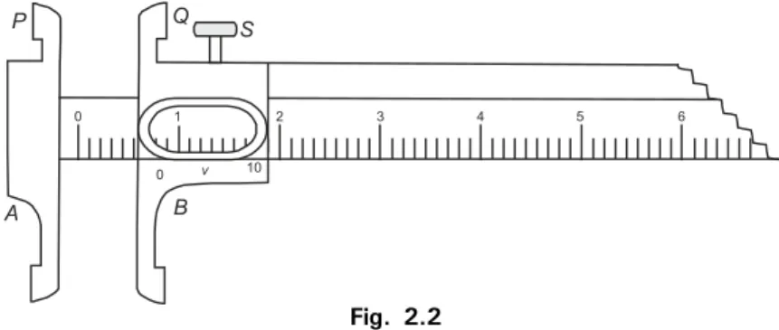
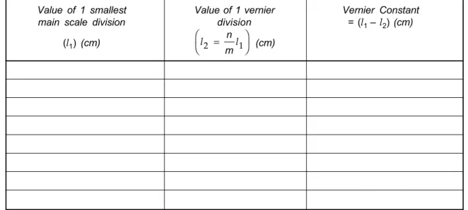
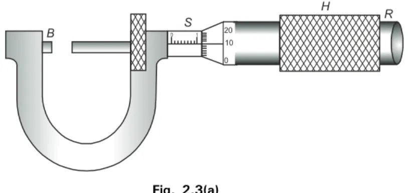
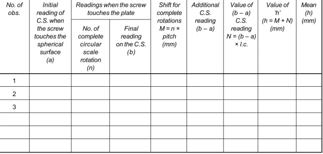
Figure
Documents relatifs
the components of a position vector with respect to a coordinate system, the scalar product of two vectors, the transformation of the components upon a change of the coordinate
The adequate framework is given by quantum electrodynamics, a quantum field theory, which combines classical electrodynamics and relativistic quantum mechanics. By subtracting
Consider a spherical electromagnetic wave propagating with a speed c with respect to a stationary frame of reference, as shown in figure 1.9.. The speed
It is because of these properties that Hermitean operators place a central role in quantum mechanics in that the observable properties of a physical system such as posi- tion,
The problem is to find the combination of the column vectors on the left side that produces the vector on the right side!. The unknowns are the numbers x and y that multiply the
For example, the Hydrogen atom in three dimensions has 3 coordinates for the internal problem, (the vector displacement between the proton and the electron). We will need three
(iii) Zero error and correction: When the zero mark of the circular scale and the main scale do not coincide on bringing the studs in contact the instrument has zero error?. The
The set of all possible outputs of a matrix times a vector is called the column space (it is also the image of the linear function defined by the matrix).. Reading homework:
