HAL Id: hal-01377379
https://hal.inria.fr/hal-01377379
Submitted on 21 Oct 2016
HAL is a multi-disciplinary open access archive for the deposit and dissemination of sci-entific research documents, whether they are pub-lished or not. The documents may come from teaching and research institutions in France or abroad, or from public or private research centers.
L’archive ouverte pluridisciplinaire HAL, est destinée au dépôt et à la diffusion de documents scientifiques de niveau recherche, publiés ou non, émanant des établissements d’enseignement et de recherche français ou étrangers, des laboratoires publics ou privés.
years of research
Ivo Ihrke, John Restrepo, Lois Mignard-Debise
To cite this version:
Ivo Ihrke, John Restrepo, Lois Mignard-Debise. Principles of Light Field Imaging: Briefly revisiting 25 years of research. IEEE Signal Processing Magazine, Institute of Electrical and Electronics Engineers, 2016, 33 (5), pp.59-69. �10.1109/MSP.2016.2582220�. �hal-01377379�
Light field imaging offers powerful new capabilities through sophisticated digital processing techniques that are tightly merged with unconventional optical designs. This combination of imaging technology and computation encompasses a fundamentally different view on the optical properties of imaging systems and poses new challenges in the traditional signal and image processing domains. In this article, we aim at providing a comprehensive review of the considerations involved and the difficulties encountered in working with light field data.
I. INTRODUCTION
As we are approaching the 25th anniversary of digital light field imaging [1], [2], [3] and the technology is entering the industrial and consumer markets, it is time to reflect on the developments and trends of what has become a vibrant inter-disciplinary field that is joining optical imaging, image processing, computer vision, and computer graphics.
The key enabling insight of light field imaging is that a re-interpretation of the classic photographic imaging procedure that is separating the process of imaging a scene, i.e. scene capture, from the actual realization of an image, i.e. image synthesis, offers a new flexibility in terms of post-processing. The underlying idea is that a digital capture process enables intermediate processing far beyond simple image processing. In fact, our modern cameras are powerful computers that enable the execution of sophisticated algorithms in order to produce high-quality 2D images.
Light field imaging is, however, moving beyond that level by purposefully modifying classical optical designs such as to enable the capture of high-dimensional data-sets that contain rich scene information. The 2D images that are presented to the human observer are processed versions of the higher-dimensional data that the sensor has acquired and that only the computer sees in its raw form. This partial replacement of physics by computation enables the post-capture modification of images on a previously unimaginable scale. Most of us will have seen the amazing features that light field cameras offer: post-capture re-focus, change of view point, 3D data extraction, change of focal length, focusing through occluders, increasing the visibility in bad weather conditions, improving the robustness of robot navigation, to name just a few.
In optical design terms, light field imaging presents an (as of yet unfinished) revolution: Since Gauss’ days, optical designers have been thinking in terms of two conjugate planes, the task of the designer being to optimize a lens system such as to gather the light originating at a point at the object plane and to converge it as well as possible to a point in the image plane. The larger the bundle of rays that can be converged accurately, the more light efficient the capture process becomes and the higher the achievable optical resolution. The requirement of light-efficient capture introduces focus into the captured images, i.e. only objects within the focal plane appear sharp. Light field imaging does away with most of these concepts, purposefully imaging out-of-focus regions and inherently aiming at capturing the full 3D content of a scene.
In terms of signal processing, we encounter a high-dimensional sampling problem with non-uniform and non-linear sample spacing and high-dimensional spatio-directionally varying observation/sampling kernels. The light field data, however, has particular structures, which can be exploited for analysis and reconstruction. This structure is caused by the fact that scene geometry and reflectance are linking the information contained in different samples. It also distinguishes the reconstruction problem from a classical signal processing task. On the software side, we witness the convergence of ideas from image processing, computer vision and computer graphics. In particular, the classical pre-processing tasks of demosaicking, vignetting compensation, undistortion, and color enhancement are all affected by sampling in four dimensions rather than in two. In addition, image analysis by means of computer vision techniques becomes an integral part of the imaging
process. Depth extraction and super-resolution techniques enhance the data and mitigate the inherent resolution trade-off that is introduced by sampling two additional dimensions. A careful system calibration is necessary for good performance. Computer graphics ideas, finally, are needed to synthesize the images that are ultimately presented to the user.
This article aims at presenting a review of the principles of light field imaging and the associated processing concepts, while simultaneously illuminating the remaining challenges. The presentation roughly follows the acquisition and processing chain from optical acquisition principles to the final rendered output image. The focus is on single camera snapshot technologies that are currently seeing a significant commercial interest.
II. BACKGROUND
The current section provides the necessary background for the remainder of the article, following closely the original development in [2]. An extended discussion at an introductory level can, e.g. be found in [4]. A wider perspective on computational cameras is given in [5], [6].
A. Plenoptic Function.
The theoretical background for light field imaging is the plenoptic function [7], which is a ray-optical concept assigning a radiance value to rays propagating within a physical space. It considers the usual three-dimensional space to be penetrated by light that propagates in all directions. The light can be blocked, attenuated or scattered while doing so.
However, instead of modeling this complexity like e.g. computer graphics is doing, the plenoptic function is an unphysical, model-less, purely phenomenological description of the light distribution in the space. In order to accommodate for all the possible variations of light without referring to an underlying model, it adopts a high-dimensional description: arbitrary radiance values can be assigned at every position of space, for every possible propagation direction, for every wavelength, and for every point in time. This is usually denoted as lλ(x, y, z, θ, φ, λ, t), where lλ[W/m2/sr/nm/s] denotes spectral radiance per unit time, (x, y, z) is a spatial
position, (θ, φ) an incident direction, λ the wavelength of light, and t a temporal instance.
The plenoptic function is mostly of a conceptual interest. From a physical perspective, the function cannot be an arbitrary 7-dimensional function since, e.g. radiant flux is delivered in quantized units, i.e. photons. Therefore, a time-average must be assumed. Similarly, it is not possible to measure infinitely thin pencils of rays, i.e. perfect directions, or even very detailed spatial light distributions without encountering wave effects. We may therefore assume that the measurable function is band-limited and that we are restricted to macroscopic settings where the structures of interest are significantly larger than the wavelength of light.
B. Light Fields.
Light fields derive from the plenoptic function by introducing additional constraints.
i They are considered to be static even though video light fields have been explored [8] and are becoming increasingly feasible. An integration over the exposure period removes the temporal dimension of the plenoptic function.
ii They are typically considered as being monochromatic, even though the same reasoning is applied to the color channels independently. An integration over the spectral sensitivity of the camera pixels removes the spectral dimension of the plenoptic function.
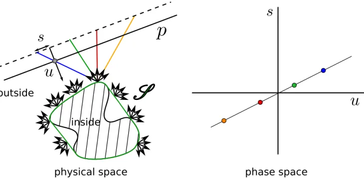
iii Most importantly, the so called free-space assumption introduces a correlation between spatial positions: Rays are assumed to propagate through a vacuum without objects except for those contained in an “inside” region of the space that is often called a scene. Without a medium and without occluding objects, the radiance is constant along the rays in the “outside” region. This removes one additional dimension from the plenoptic function [2].
A light field is therefore a four-dimensional function. We may assume the presence of a boundary surfaceS that is separating the space into the “inside” part, i.e. the space region containing the scene of interest, and the “outside” part where the acquisition apparatus is located. The outside is assumed to be empty space. Then the light field is a scalar valued function on S × S+2, where S+2 is the hemisphere of directions towards the
inside
outside
physical space
phase space
Fig. 1. Light field definition. (left) The “inside” region contains the scene of interest, the “outside” region is empty space and does not affect light propagation. The light field is a function assigning a radiance value to each of the rays exiting through the boundary surfaceS . (right) A phase space illustration of the colored rays. A point in phase space determines a set of ray parameters (u, s) and therefore corresponds to a ray. The phase space is associated with the plane p. Since the 4 rays indicated in the left sub-figure converge to a point, the corresponding phase space points lie on a line.
outside. This definition of a light field is also know as a “surface light field” [9] if the surface S agrees with some object geometry. In this case, the directional component of the function describes the object reflectance convolved with the incident illumination.
Commonly, the additional assumption is made that the surfaceS is convex, e.g. by taking the convex hull of the scene. In this case, the rays can be propagated to other surfaces in the “outside” region without loss of information. Typically, a plane p is used as the domain of (parts of) the light field function. The most popular parameterization of the spatial and directional dimensions of the light field is the “two-plane parameterization”. It is obtained by propagating a ray from surface S to the light field plane p, see Fig. 1. The parameterization then consists of the intersection position (u, v) of the ray with the light field plane p and its intersection with an additional parallel plane at a unit distance (ˆu, ˆv). The second intersection is usually parameterized as a difference with respect to the (u, v) position and called (s = ˆu − u, t = ˆv − v). This second set of coordinates measures the direction of the ray.
Fig. 1, as all of the following figures, only shows one spatial dimension u and one directional dimension s.
C. Phase Space.
The coordinates obtained this way can be considered as an abstract space, the so-called “ray phase space”, or simply phase space. A point (u, v, s, t) in this space corresponds to a ray in the physical space. It is important to remember that the phase space is always linked to a particular light field plane p. Changing the plane, in general, changes the phase space configuration, which means that a fixed ray will be associated with a different phase space point.
The phase space is interesting for several reasons. First, it allows us to think more abstractly about the light field. Second, a reduction to two dimensions (u, s) is easily illustrated and generalizes well to the full four-dimensional setting. Third, finite regions of the ray space, in contrast to infinitesimal points, describe ray bundles. The phase space is therefore a useful tool to visualize ray bundles. Finally, there is a whole literature on phase space optics, see e.g. [10] with available extensions to wave optics. The phase space is also a useful tool for comparing different camera designs [11].
meaning that each ray, parameterized by (u, v, s, t) is assigned a radiance value l. The task of an acquisition system is to sample and reconstruct this function.
D. Light Field Sampling.
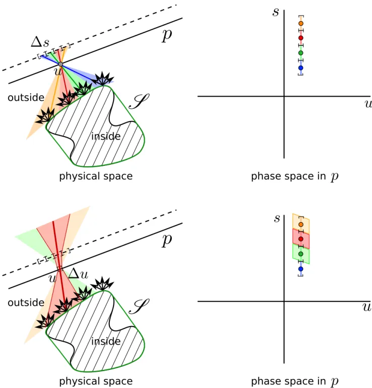
The simplest way of sampling the light field function is by placing a pinhole aperture into the light field plane p. If the pinhole was infinitesimal, ray optics was a decent model of reality, and light considerations were negligible, we would observe one column of the light field function at a plane a unit distance from the light field plane p. In the following we will refer to that plane as the sensor plane q. Associating a directional sample spacing of ∆s, and shifting the pinhole by amounts of ∆u, enables a sampling of the function, Fig. 2. A slightly more realistic model is that the directional variation s is acquired by finite-sized pixels with a width equivalent to the directional sample spacing ∆s. This introduces a directional sampling kernel, which in phase space can be interpreted as a vertical segment, Fig. 2 (top). Of course, the pinhole has a finite dimension ∆u, too. The pinhole/pixel combination therefore passes a bundle of rays as indicated in Fig. 2 (bottom left). The phase space representation of the ray bundle passing this pinhole/pixel pair is a sheared rectangle as shown in Fig. 2 (bottom right). It should be noted that the pinhole size and the pinhole sample spacing, as well as the pixel size and the pixel spacing, may not be correlated in real applications, with the corresponding implications for aliasing or over-sampling, Sect. V.
Going back to the physical meaning of these phase space regions, respective ray bundles, we can conclude that each pinhole/pixel combination yields a single measurement, i.e. a single sample of the light field function through integration by the pixel. The phase space region therefore represents the spatio-directional sampling kernel introduced by the finite size of the pixel and the pinhole, respectively, while the center ray/phase space point indicates the associated sampling position.
A key optical concept, the optical invariant states that an ideal optical system does not change the volume of such a phase space region, also known as ´etendue. As an example, free-space transport, as a particularly simple propagation maintains phase space volume. It is described by a shear in the horizontal direction of the phase space. Free-space transport to a different plane is a necessary ingredient for computing refocused 2D images from the light field.
E. Light Field Sampling with Camera Arrays / Moving Cameras
Obviously, pinhole images are of a low quality due to blurring by the finite pinhole area, or, depending on its size, diffraction effects, and due to the low light through-put. Introducing a lens in the light field plane p improves the situation. This measure has the side effect of moving the apparent position of the sensor plane q in front of the light field plane p if the sensor is positioned at a farther distance than the focal length of the lens, see Fig. 3. The ray bundles that are being integrated by a single pixel can still be described by a two-aperture model as before; however, at this point the model must be considered virtual. This implies that it may intersect scene objects. It is understood that the virtual aperture does not affect the scene object in any way. The key point is that the refracted rays in the image space of the lens can be ignored as a means of simplifying the description. Only the ray bundles in the world space that are being integrated by the pixel are considered.
With this change, the sampling of the light field remains the same as before: Instead of moving a pinhole, a moving standard 2D camera performs the sampling task. Only the parameterization of the directional component s needs to be adapted to the camera’s intrinsic parameters. This is how pioneering work was performed [2], [3]. Of course, this acquisition scheme can be implemented in a hardware-parallel fashion by means of camera arrays [8], [12].
Given a sampled light field l(u, v, s, t), and assuming full information to be available, the slices I(s, t) = l(u = const., v = const., s, t) as well as I(u, v) = l(u, v, s = const., t = const.) correspond to views into the scene. The function I(s, t) corresponds to a perspective view, whereas I(u, v) corresponds to an orthogonal view of the “inside” space. These views are often referred to as light field subviews.
inside
outside
physical space
phase space in
inside
outside
physical space
phase space in
Fig. 2. Finite sampling of a light field with real hardware. (Top) Assuming a sensor placed at the dashed plane and an infinitesimal pinhole results in a discretization and averaging of only the directional light component. In phase space, this constitutes a row of vertical segments. (Bottom) A more realistic scenario uses a finite-sized pinhole, resulting in ray bundles that are being integrated by the pixels of the sensor. Pixels and pinholes, in conjunction, define a two-aperture model. In phase space, the ray bundle passed by two apertures is represented by a rhomb.
inside
outside
physical space
real sensor plane
virtual sensor plane
image of
a pixel
pixel
Fig. 3. Light field imaging with a moving standard camera. Sensor pixels in the sensor plane q are mapped outside of the camera and inside the world space. The camera lens and the image of the pixel constitute a two-aperture pair, i.e. a unique phase space region. The color gradient in the ray bundle indicates that the rays are considered to be virtual in the image space of the camera. In reality, the rays refract and are converged onto the indicated pixel. In world space, the ray bundle represents those rays that are integrated by the pixel. The sensor has more such pixels which are not shown in the figure. These additional pixels effectively constitute a moving aperture in the plane of the virtual sensor position.
III. OPTICS FORLIGHTFIELD CAMERAS
While camera arrays can be miniaturized as demonstrated by Pelican Imaging Corp. [12], and differently configured camera modules may be merged as proposed by LightCo. Inc. [13], there are currently no products for end-users and building and maintaining custom camera arrays is costly and cumbersome.
In contrast, the current generation of commercial light field cameras by Lytro Inc. [14] and Raytrix GmbH [15] has been built around in-camera light field imaging, i.e. light field imaging through a main lens. In addition, there are attempts at building light field lens converters [16] or using mask-based imaging systems [17] that can turn standard SLR cameras into light field devices. All devices for in-camera light field imaging aim at sampling a light field plane p inside the camera housing.
To understand the properties of the in-camera light field and their relation to the world space, the previous discussion of general light field imaging will now be extended to the in-camera space.
A. In-Camera Light Fields.
In this setting, the light field is transformed from world space into the image space of a main lens, where it is being acquired by means of miniature versions of the camera arrays outlined above that are most often practically implemented using micro-optics mounted on a single sensor. The commercial implementations involve microlenses mounted in different configurations in front of a standard 2D sensor. Each microlens with its underlying group of pixels forms an in-camera (u, v, s, t) sampling scheme just as described in Sect. II. We may also think about them as tiny cameras with very few pixels that are observing the in-camera light field. The image of a single microlens on the sensor is often referred to as a micro-image.
camera
main lens
light
field
plane
sensor
plane
virtual
sensor
plane
(world)
light field
plane
(world)
virtual
sensor
plane
(in-camera)
micro-camera
array
(real)
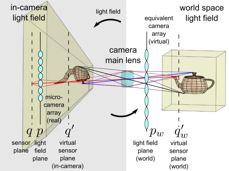
Fig. 4. The main lens is imaging its object space (right) into its image space (left), distorting it in the process. The world space light field is therefore distorted into an in-camera light field. The distortion is a perspective projection with its center at the center of the image space principal plane of the main lens. A micro-optics implementation of a camera array is observing the distorted in-camera light field. An equivalent camera array in world coordinates can be found by mapping the light field plane p and the virtual sensor plane q0 to the world space.
Unfortunately, the in-camera light field is a distorted version of the world coordinate light field due to refraction by the main lens. Here, we encounter a classical misconception: Mapping the world space into the image space of the main lens, even by means of a simple thin-lens transformation, does not result in a uniformly scaled version of the world space. Instead, the in-camera light field is a projectively distorted version of the world space light field, see Fig. 4. The underlying reason is the depth-dependent magnification of optical systems.
There are different ways to describe this distortion, e.g. in terms of phase space coordinates as suggested by Dansereau et al. [18] which corresponds to a ray-remapping scheme, or by appropriate projection matrices. The projection matrices commonly used in computer vision to model camera intrinsics and extrinsics are not directly usable since they model a projection onto the image plane of a 2D camera. It is, however, important that 3D information is preserved. The closest model are the OpenGL projection matrices used in computer graphics that transform a Euclidean world space into a space of so-called Normalized Device Coordinates. This space is also a 3D space, but a perspectively distorted one.
B. Interpreting In-Camera Light Field Imaging in World Space.
Thinking about how a miniature camera array is imaging the distorted in-camera light field is a bit difficult. It is, however, possible to apply the inverse perspective transformation to the light field plane and the virtual
sensor plane, i.e. to the two aperture planes that are characterizing a light field sampling device, to obtain a world space description in terms of an equivalent camera array.
The detailed position of these two planes depends on the configuration of the light field camera. There are essentially two choices:
a) an afocal configuration of the lenslets [19], and b) a focussed configuration of the lenslets [20], [15].
For option a), the sensor plane is positioned exactly at the focal distance of the microlens array. In option b) there are the two possibilities of creating real or virtual imaging configurations of the micro-cameras by putting the sensor plane farther or closer than the microlens focal length, respectively. This choice has the effect of placing the in-camera virtual sensor plane at different positions, namely at infinity for option a), or in the front or in the back of the microlens plane for option b).
In practice, option a) can only be approximately achieved. First, it is difficult to mechanically set the sensor at the right distance from the microlens array. Second, since a microlens is often a one lens system, its focal length is strongly dependent on the wavelength of the light. The configuration may be set for green light but the red and blue wavelengths are then focused at different distances. The finite pitch of the pixels, however, makes the system tolerant to these issues.
In microlens based light field imaging, the microlens plane takes the role of the in-camera light field plane p. The virtual sensor plane, i.e. the sensor plane transformed by the microlens array takes the role of the second aperture as in Fig. 3.
The inverse action of the main lens is then to map these two planes into world space. In conjunction, they define the properties of the light field sub-views such as focal plane, depth-of-field, viewing direction and angle, field-of-view, and, through these parameters, the sampling pattern for the world-space light field. Optically refocusing the main lens, i.e. changing its position with respect to the microlens array, affects most of these properties. The precise knowledge of the optical configuration is therefore necessary for advanced image processing tasks such as super-resolution and corresponding calibration schemes have been developed, Sect. IV.
C. Optical Considerations for the Main Lens
The main optical considerations are concerning the (image-side) f-number of the main lens and the (object-side) f-number of the microlenses respectively. The f-number of an imaging system is the ratio of its focal length and the diameter of its entrance pupil. It describes the solid angle of light rays that are passed by an optical system. The f-number is an inverse measure, i.e. larger f-numbers correspond to smaller solid angles. For in-camera light field systems, the f-number of the main lens must always be larger than that of the microlenses in order to ensure that light is not leaking into a neighboring micro-camera. At the same time, for a good directional sampling, the f-number should be as small as possible. Ideally, the main lens f-number would remain constant throughout all operation conditions. This requirement puts additional constraints, especially on zoom-systems [21].
The discussion so far has involved ideal first-order optics. In reality, optical systems exhibit aberrations, i.e. deviations from perfect behavior. Initial investigations [22] have shown that the phase space sampling patterns are deformed by the main lens aberrations. In addition to the classical distinction between geometric and blurring aberrations, an interpretation of the phase space distortions yields that directional shifts, i.e. a directional variant of the geometric distortions, and directional blur, i.e. a mixture of sub-view information are introduced by aberrated main lenses. The effects of microlens aberrations are relatively minor and only concern the exact shape of the sampling kernel.
An example of the distortions introduced by an aberrated main lens, as opposed to an ideal thin lens, are illustrated in Fig. 5. The horizontal shifts in the sampling patterns correspond to geometric distortion, typically treated by radial distortion models [18], [23]. The (slight) vertical shifts correspond to a directional deformation of the light field subviews.
A known shifting pattern can be used to digitally compensate main lens aberrations [22], or to even exploit the effect for improving light field sampling schemes [24], see also Sect. V.
-0.5 0 0.5 -0.1 -0.08 -0.06 -0.04 -0.02 0 -0.5 0 0.5 -0.1 -0.08 -0.06 -0.04 -0.02 0
thin lens
raytrace
u
A.U.u
A.U. A .U. A .U. Double Gauss f/4Fig. 5. Effect of lens aberrations for an f/4 afocal light field system: (left) Phase space distribution of the sampling pattern in world space, assuming an ideal main lens (thin lens). (right) Phase space distribution of the sampling pattern in world space using an f/4 Double Gauss system as a main lens. The sampling pattern is significantly distorted. The highlighted phase space regions correspond between the left and the right plots. The side subview (purple) is more severly affected as compared to the center subview (blue).
While a satisfactory treatment of first-order light field imaging can be achieved by trigonometric reasoning or updated matrix optics techniques, a complete theory of light field aberrations is missing at the time of writing.
IV. CALIBRATION ANDPREPROCESSING
Preprocessing and calibration are tightly interlinked topics for light field imaging. As outlined in the previous section, many parameters of a light field camera change when the focus of the main lens is changed. This not only concerns the geometric characteristics of the views, but also their radiometric properties. The preprocessing of light field images needs to be adapted to account for these changes. In addition, different hardware architectures require adapted pre-processing procedures. We will therefore cover the steps only in an exemplary manner. The underlying issues, however, affect all types of in-camera light field systems. Our example uses a Lytro camera, which is an afocal lenslet-based light field imaging system.
A. Color Demosaicking
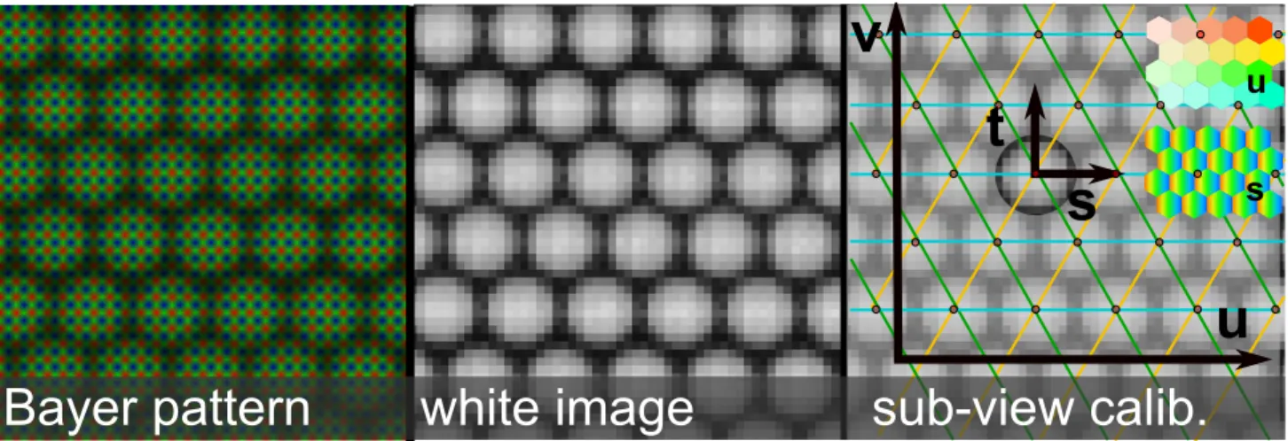
Using a standard Bayer color filter array to enable colored light field imaging appears to be a straight-forward choice. However, as shown in Fig. 6 (right) for the case of an afocal light field camera, each micro-image encodes the (s, t) dimensions of the light field. Different color channels therefore correspond to different (s, t) sampling patterns. The final image quality can be improved when taking this fact into account [25].
B. Vignetting
The intensity fall-off towards the sides of the micro-images, also known as vignetting, changes with the optical settings of the main lens. Commercial cameras therefore store significant amounts of calibration information in the internal camera memory. As an example, the combined vignetting of main lens and microlenses changes across the field of view and with focus and zoom settings of the main lens. Therefore, white images have to be taken for a sufficiently dense set of parameter settings. The closest white image to the parameters of a user shot are then used for compensation. In a lab setting, it is advisable to take one’s own white images prior to data acquisition.
u
v
s
t
s
u
white image
sub-view calib.
Bayer pattern
Fig. 6. Light field pre-processing and calibration for a Lytro camera: (left) Using a Bayer pattern within the micro-images causes a shift of light-field view for the color channels since different colors sample different (s, t) coordinates. (middle) white image (luminance) used for vignetting compensation, (right) A sub-pixel determination of the centers of the micro-images enables a calibrated (s, t)-coordinate system to be assigned to each micro-image. The (u, v) t)-coordinates are sampled in a hexagonal fashion by the microlenses. The orientation of this global coordinate system also determines the rotation angle of the (s, t) system. The inset shows s and u calibration maps for the raw image.
C. Calibration
In order to properly decode the four light field dimensions from the 2D sensor image, it is necessary to carefully calibrate the (u, v, s, t) coordinates of every pixel that has been recorded by the sensor. With current lenslet-based architectures, to first order, this amounts to determining the center positions of the lenslets, and the layout of the lenslet grid, Fig 6 (right). More accurately, the position of the central view is given by the sensor intersection of chief rays passing through the main lens and each one of the lenslets. In addition, microlens aberrations and angularly variable pixel responses can shift this position [26]. In general, the responses are also wavelength dependent.
The lenslet grid is typically chosen to be hexagonal in order to increase the sensor coverage. The spherical shape of the micro-images and their radius are determined by the vignetting of the main lens which is due to its aperture size and shape. The tight packing of the micro-images is achieved by f-number matching as discussed in Sect. III. It should also be noted that manufacturing a homogeneous lenslet array is difficult and some variation may be expected. Further, the mounting of the lenslet array directly on the sensor may induce a variable distance between the sensor and the lenslets.
The calibration described above usually pertains to the in-camera light-field coordinates. When assuming thin-lens optics for the main lens, these correspond to a linear transformation of the light field coordinates in object space. Calibration approaches to determine this mapping are described by Dansereau et al. [18] for afocal light field cameras. The techniques, as well as the pre-processing steps described above, are implemented in his MATLAB Light Field Toolbox. Bok et al [27], present an alternative to perform a similar calibration, by directly detecting line features of a calibration target from the raw light field images. Johannsen et al. [23] describe the calibration scheme for focussed light field cameras. The handling of the effects of optical aberrations by the main lens is usually performed using classical radial distortion models from the computer vision literature. While these measures improve the accuracy, they are not completely satisfactory since the light field subviews suffer from non-radial distortions, see Fig. 5 (right). Lytro is providing access to calibration information including aberration modeling through its SDK. Alternatively, model-less per-ray calibrations [28] using structured light measurements have shown promising performance improvements. However, the need for a principled distortion model remains.
Once a per-pixel calibration is known, the suitably pre-processed radiance values of the light field function can be assigned to a sample position in phase space. In principle, reconstructing the full light field function amounts to a signal processing task: given a set of irregular samples in phase space, reconstruct the light field function on that space. In practice, additional constraints apply and are used to e.g. achieve super-resolution or to extract depth. A prerequisite for super-resolution is a known shape of the phase space sampling kernels,
light field subview (u,v)=const.
light field epi (v,t)=const.
s
t
s
u
Fig. 7. Light field subview and epipolar plane image (EPI) corresponding to the green line in the subview. The images represent different slices of the four-dimensional light field function l(u, v, s, t). Note the linear structures of constant color in the EPI. These structures correspond to surface points. Their slope is related to the depth of the scene point.
also known as ray-spread functions. Calibration schemes for these still have to be developed.
V. COMPUTATIONALPROCESSING
The reconstruction of the four-dimensional light field function from its samples can be achieved by standard interpolation schemes [2], [29]. However, the light field function possesses additional structure. It is not an arbitrary four-dimensional function, but its structure is determined by the geometry and radiometry of the scene.
As an example, if the sampled part of the light field plane pw is small with respect to the distance to an
object point within the “inside” region, then the solid angle of the system aperture with respect to the surface point is small. If the surface is roughly Lambertian, the reflectance does not vary significantly within this solid angle and can be assumed constant. This restriction often applies in practice and the “mixed” positional-directional slices of the light field function, e.g. l(u, v = const., s, t = const.), show a clear linear structure, see Fig. 7. These images are also known as epipolar plane images or EPIs with reference to the epipolar lines of multiple view computer vision. In case of non-Lambertian surfaces, the linear structures carry reflectance information that is convolved with the illumination.
Assuming the constancy of the light field function along these linear structures to be a valid approximation, and considering the four-dimensional case instead of our two-dimensional illustrations, i.e. planar structures instead of linear ones corresponding to geometric scene points, we see that the intrinsic dimensionality of the light field is only 2D in the Lambertian case. In practice it is necessary to have a knowledge of scene depth to exploit this fact. On the other side, the constraint serves as a basis for depth estimation. This observation is the basis for merging the steps of reconstructing the light field function (signal processing), depth reconstruction (computer vision), and super-resolution (image processing). More general constraints are known. As an example, Levin et al. [30] proposed a 3D constraint in the Fourier domain that works without depth estimation.
Intuitively, the linear structure implies that the surface point corresponding to a sloped line can be brought into focus, which in phase space is a shear in the horizontal direction, see also Fig. 1. Focus is achieved when the sloped line becomes vertical. In this case, there is only angular information from the surface point, which implies that its reflectance (convolved with the incident illumination) is being acquired. The amount of shear that is necessary to achieve this focusing is indicative of the depth of the scene point with respect to the light field plane pw. The slope of the linear structures is therefore an indicator for depth.
A. Depth Estimation
In light of the above discussion, depth estimation is a first step towards super-resolution. It amounts to associating a slope with every phase space sample [11]. There are several ways to estimate depth in light fields. The standard way is to extract light field subviews and to perform some form of multi-view stereo estimation. Popular techniques such as variational methods [31], [16] or graph-cut techniques have been explored [32]. The literature on the topic is too large to review here and we recommend to consult the references provided here for further discussions.
The main difference between multi-view stereo on images from regular multi-camera arrays and for light field cameras are the sampling patterns in phase space. Whereas the sample positions and sampling kernels of multi-camera arrays are typically sparse in phase space, for light field cameras, the respective sampling patterns and kernels usually tile it. We therefore have a difference in the aliasing properties of these systems. Aliased acquisition implies the necessity for solving the matching or correspondence problem of computer vision, a notoriously hard problem. In addition, the phase space slope vectors are only estimated indirectly through (possibly inconsistent) disparity assignments in each of the subviews.
The dense sampling patterns of light field cameras allow for alternative treatments. As an example, recent work has explored the possibility of directly estimating the linear structures in the EPI images [33] based on structure tensor estimation. This technique is directly assigning the slope vectors to each point in the phase space. However, it does not model occlusion boundaries, i.e. T-junctions in the phase space and therefore does not perform well at object boundaries. Recent work is addressing this issue through estimating aperture splits [34] or exploiting symmetries in focal stack data corresponding to the light field [35].
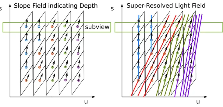
B. Super-Resolution
The knowledge of the slope function can be used to compute super-resolved light fields [36], [33] by filling the phase space with lines that have the slope and the radiance associated to a phase space sample, see Fig. 8. If the samples are jittered along the slope of the line, a geometric type of super-resolution results. This effect is used in computer graphics rendering to inexpensively predict samples for high-dimensional integration as for rendering depth-of-field effects [36]. As the samples are perfectly Dirac, and the exact depth is a byproduct of the rendering pipeline, this fact is relatively simple to exploit as compared to the corresponding tasks in light field imaging.
In working with real data, the depth needs to be estimated as described above. Since the samples are affected by the sampling kernel, i.e. the phase space regions associated with a sample, true super-resolution needs the additional step of deconvolving the resulting function [37]. For microscopic light field applications, a wave optics perspective is necessary [38], [39] and the deconvolution consequently includes wave effects.
u
u
Fig. 8. Depth Estimation and Super-Resolution: (left) Assigning a depth value to phase space samples in all sub-views assigns a slope field to the light field. This can, e.g., be achieved by matching samples between subviews as in stereo or multi-view stereo matching. (right) Propagating the radiance values of the samples along the slope field generates a super-resolved light field and therefore super-resolved subviews. Since the samples represent a convolution with the sampling kernel, a deconvolution step following the line propagation improves the result. The line propagation needs to consider occlusion (T-junctions).
C. A Note on Aliasing
A common statement in the literature is that an aliased acquisition is required for super-resolution [37]. In light of the above discussion, we may make this statement more precise by stating that a) a Lambertian scene model is implied for geometric super-resolution, b) the samples should be jittered along the slope corresponding to a scene point’s depth, and c) smaller phase space kernels associated with the samples will be beneficial as long as there is still overlap between them when propagated along the lines to construct the super-resolved sub-view. In conclusion, light field cameras may be more suitable to implement super-resolution schemes than multi-camera arrays due to their denser sampling of the phase space.
VI. IMAGESYNTHESIS
Once the light field function is reconstructed, novel 2D views can be synthesized from the data. The simplest visualization is to extract the light field subviews, i.e. images of constant (u, v) or (s, t) coordinates depending on the sampling pattern of the specific hardware implementation. It should be noted that both choices, in general yield perspective views. This is because in-camera orthographic views (as synthesized by fixing the (s, t) coordinates) map to a world space center of projection in the focal plane of the main lens. The subviews correspond to the geometry of the world space light field plane pw and the world space virtual
sensor plane q0w and therefore show a parallax between views. Interpolated subview synthesis has been shown to benefit from depth information [40]: available depth information, even if coarse, enables aliasing-free view synthesis with less subviews.
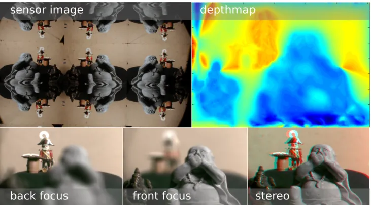
The goal of light field image synthesis, however, is the creation of images that appear as if they were taken by a lens system that was not physically in place, see Fig. 9. The example most commonly shown is synthetic refocusing [29]. The technique, in its basic form, consists in performing a free-space transport of the world space light field plane to the desired focus plane. After performing this operation, an integral over the directional axis of the light field, i.e. along the vertical dimension in our phase space diagrams, yields a 2D view that is focused at the selected plane. Choosing only a sub-range of the angular domain lets the user select an arbitrary aperture setting, down to the physical depth-of-field present in the light field subviews
sensor image
depthmap
back focus
front focus
stereo
Fig. 9. Light field image synthesis. (top left) A raw image from the optical light field converter of Manakov et al. [16], (top right) depth map for the center view, computed with multi-view stereo techniques, (bottom row) a back and front focus using extrapolated light fields to synthesize an f/0.7 aperture (physical aperture f/1.4), (bottom right) a synthesized stereo view with user-selectable baseline.
that is determined by the sizes of the two (virtual) apertures that are involved in the image formation. If spatio-directional super-resolution techniques, as in Sect. V, are employed, this limit may be surpassed.
Computing the four-dimensional integral allows for general settings – even curved focal planes are possible by selecting the proper phase space sub-regions to be integrated. However, it can be computationally expensive. If the desired synthetic focal plane is parallel to the world space light field plane pw, and the angular integration
domain is not restricted, Fourier techniques can yield significant speed-ups [14]. If hardware accelerated rendering is available, techniques based on texture-mapped depthmaps can be efficient alternatives [16].
VII. CONCLUSIONS
With almost a quarter century of practical feasibility, light field imaging is up and well, gaining popularity and progressing into the markets with several actors pushing for prime time. There are still sufficiently many scientific challenges to keep researchers occupied for some time to come. In particular, the bar of resolution loss must still be lowered in hope of increased consumer acceptance. The mega-pixel race has slowed down and pixel sizes are approaching their physical limits. This implies larger sensors and thus increased expense for additional resolution increases that would benefit light field technology. Improved algorithmic solutions are therefore of fundamental importance. The next big step will be light field video, pushing optical flow towards scene flow and the associated projected applications like automatic focus pulling, foreground/background segmentation, space-time filtering, etc. In terms of applications, we are seeing 4D light field ideas penetrating towards the small and the large. In the small, we are seeing the emergence of Light Field Microscopy [41], though we need improved aberration models and eventually expanded wave-optical treatments [39]. In the large, sensor networks will become increasingly important. More complex scenes are made possible, like translucent objects [42] or more generally non-lambertian scenes [43]. Cross-over to other fields as Physics are appearing [44]. These are surely exciting times as we are heading into the second quarter century of light field technology.
REFERENCES
[1] E. H. Adelson and J. Y. A. Wang, “Single Lens Stereo with a Plenoptic Camera,” IEEE Trans. PAMI, no. 2, pp. 99–106, 1992. [2] M. Levoy and P. Hanrahan, “Light Field Rendering,” in Proc. SIGGRAPH, 1996, pp. 31–42.
[3] S. J. Gortler, R. Grzeszczuk, R. Szeliski, and M. F. Cohen, “The Lumigraph,” in Proc. SIGGRAPH, 1996, pp. pp. 43–54. [4] M. Levoy, “Light Fields and Computational Imaging,” IEEE Computer, vol. 39, no. 8, pp. 46–55, 2006.
[5] C. Zhou and S. K. Nayar, “Computational cameras: Convergence of optics and processing,” IEEE Trans. IP, 2011.
[6] G. Wetzstein, I. Ihrke, D. Lanman, and W. Heidrich, “Computational Plenoptic Imaging,” CGF, vol. 30, no. 8, pp. 2397–2426, oct 2011.
[7] E. H. Adelson and J. R. Bergen, “The Plenoptic Function and the Elements of Early Vision,” in Computational Models of Visual Processing. MIT Press, 1991.
[8] B. Wilburn, N. Joshi, V. Vaish, E.-V. Talvala, E. Antunez, A. Barth, A. Adams, M. Horowitz, and M. Levoy, “High Performance Imaging using Large Camera Arrays,” ACM TOG, vol. 24, no. 3, pp. 765–776, 2005.
[9] D. N. Wood, D. I. Azuma, K. Aldinger, B. Curless, T. Duchamp, D. H. Salesin, and W. Stuetzle, “Surface Light Fields for 3D Photography,” in Proc. SIGGRAPH, 2000, pp. 287–296.
[10] A. Torre, Linear Ray and Wave Optics in Phase Space. Elsevier, 2005.
[11] A. Levin, W. T. Freeman, and F. Durand, “Understanding Camera Trade-Offs through a Bayesian Analysis of Light Field Projections,” in Proc. ECCV, 2008, pp. 88–101.
[12] K. Venkataraman, D. Lelescu, J. Duparr´e, A. McMahon, G. Molina, P. Chatterjee, R. Mullis, and S. Nayar, “PiCam: An Ultra-thin High Performance Monolithic Camera Array,” ACM TOG, vol. 32, no. 6, p. article 166, 2013.
[13] R. Laroia, “Zoom Related Methods and Apparatus,” US Patent Application 14/327,525, 2014. [14] R. Ng, “Fourier Slice Photography,” ACM TOG, vol. 24, no. 3, pp. 735–744, 2005.
[15] C. Perwass and L. Wietzke, “Single Lens 3D-Camera with Extended Depth-of-Field,” in Proc. SPIE vol. 8291, Human Vision and Electronic Imaging XVII, 2012, p. 829108.
[16] A. Manakov, J. F. Restrepo, O. Klehm, R. Heged¨us, E. Eisemann, H.-P. Seidel, and I. Ihrke, “A Reconfigurable Camera Add-on for High Dynamic Range, Multispectral, Polarization, and Light-Field Imaging,” ACM TOG, vol. 32, no. 4, p. article 47, 2013. [17] A. Veeraraghavan, R. Raskar, A. Agrawal, A. Mohan, and J. Tumblin, “Dappled Photography: Mask Enhanced Cameras For
Heterodyned Light Fields and Coded Aperture Refocussing,” ACM TOG, vol. 26, no. 3, p. article 69, 2007.
[18] D. G. Dansereau, O. Pizarro, and S. B. Williams, “Decoding Calibration and Rectification for Lenselet-Based Plenoptic Cameras,” in Proc. CVPR, 2013, pp. 1027–1034.
[19] R. Ng, M. Levoy, M. Br´edif, G. Duval, M. Horowitz, and P. Hanrahan, “Light Field Photography with a Hand-Held Plenoptic Camera,” Stanford University, Tech. Rep. Stanford Tech Report CTSR 2005-02, 2005.
[20] A. Lumsdaine and T. Georgiev, “The Focused Plenoptic Camera,” in Proc. ICCP, 2009, pp. 1–8.
[21] T. J. Knight, Y.-R. Ng, and C. Pitts, “Light Field Data Acquisition Devices and Methods of Using and Manufacturing Same,” US Patent 8,289,440, 2012.
[22] P. Hanrahan and R. Ng, “Digital Correction of Lens Aberrations in Light Field Photography,” in Proc. SPIE vol. 6342, International Optical Design Conference, 2006, p. 63421E.
[23] O. Johannsen, C. Heinze, B. Goldluecke, and C. Perwaß, “On the Calibration of Focused Plenoptic Cameras,” in Time-of-Flight and Depth Imaging. Sensors, Algorithms, and Applications. Springer, 2013, pp. 302–317.
[24] L.-Y. Wei, C.-K. Liang, G. Myhre, C. Pitts, and K. Akeley, “Improving Light Field Camera Sample Design with Irregularity and Aberration,” ACM TOG, vol. 34, no. 4, p. article 152, 2015.
[25] Z. Yu, J. Yu, A. Lumsdaine, and T. Georgiev, “An Analysis of Color Demosaicing in Plenoptic Cameras,” in Proc. CVPR, jun 2012, pp. 901–908.
[26] C.-K. Liang and R. Ramamoorthi, “A Light Transport Framework for Lenslet Light Field Cameras,” ACM TOG, vol. 34, no. 2, pp. 1–19, mar 2015.
[27] Y. Bok, H. G. Jeon, and I. S. Kweon, “Geometric calibration of micro-lens-based light field cameras using line features,” IEEE Transactions on Pattern Analysis and Machine Intelligence, vol. PP, no. 99, pp. 1–1, 2016.
[28] F. Bergamasco, A. Albarelli, L. Cosmo, A. Torsello, E. Rodola, and D. Cremers, “Adopting an Unconstrained Ray Model in Light-field Cameras for 3D Shape Reconstruction,” in Proc. CVPR, 2015, pp. 3003–3012.
[29] A. Isaksen, L. McMillan, and S. J. Gortler, “Dynamically Reparameterized Light Fields,” in Proc. SIGGRAPH, 2000, pp. 297–306. [30] A. Levin and F. Durand, “Linear View Synthesis using a Dimensionality Gap Light Field Prior,” in Proc. CVPR, 2010, pp.
1831–1838.
[31] S. Heber, R. Ranftl, and T. Pock, “Variational shape from light field,” in Energy Minimization Methods in Computer Vision and Pattern Recognition, 2013.
[32] H. G. Jeon, J. Park, G. Choe, J. Park, Y. Bok, Y. W. Tai, and I. S. Kweon, “Accurate Depth Map Estimation from a Lenslet Light Field Camera,” in Proceedings of the IEEE Conference on Computer Vision and Pattern Recognition, 2015, pp. 1547–1555. [33] S. Wanner and B. Goldluecke, “Variational Light Field Analysis for Disparity Estimation and Super-Resolution,” IEEE Trans.
PAMI, vol. 36, no. 3, pp. 606–619, 2014.
[34] T. C. Wang, A. A. Efros, and R. Ramamoorthi, “Occlusion-aware depth estimation using light-field cameras,” in 2015 IEEE International Conference on Computer Vision (ICCV), Dec 2015, pp. 3487–3495.
[35] H. Lin, C. Chen, S. B. Kang, and J. Yu, “Depth Recovery from Light Field Using Focal Stack Symmetry,” Proc. ICCV, pp. 3451–3459, 2015.
[36] J. Lehtinen, T. Aila, J. Chen, S. Laine, and F. Durand, “Temporal Light Field Reconstruction for Rendering Distribution Effects,” ACM TOG, vol. 30, no. 4, p. article 55, 2011.
[37] T. E. Bishop, S. Zanetti, and P. Favaro, “Light Field Superresolution,” in Proc. ICCP, 2009, pp. 1–8.
[38] S. A. Shroff and K. Berkner, “Image formation analysis and high resolution image reconstruction for plenoptic imaging systems,” Appl. Optics, vol. 52, no. 10, p. D22, 2013.
[39] M. Broxton, L. Grosenick, S. Yang, N. Cohen, A. Andalman, K. Deisseroth, and M. Levoy, “Wave optics theory and 3-D deconvolution for the light field microscope,” Optics Exp., vol. 21, no. 21, p. 25418, 2013.
[40] J.-X. Chai, S.-C. Chan, H.-Y. Shum, and X. Tong, “Plenoptic sampling,” in Proc. SIGGRAPH, 2000, pp. 307–318.
[41] M. Levoy, “Light field photography, microscopy and illumination,” in International Optical Design Conference and Optical Fabrication and Testing. Optical Society of America, 2010, p. ITuB3.
[42] Y. Xu, H. Nagahara, A. Shimada, and R.-I. Taniguchi, “TransCut: Transparent Object Segmentation from a Light-Field Image,” Proc. ICCV, pp. 3442–3450, 2015.
[43] L. Shi, H. Hassanieh, A. Davis, D. Katabi, and F. Durand, “Light Field Reconstruction Using Sparsity in the Continuous Fourier Domain,” ACM TOG, vol. 34, no. 1, pp. 1–13, dec 2014.
[44] C. Skupsch and C. Br¨ucker, “Multiple-plane particle image velocimetry using a light-field camera,” Optics Exp., vol. 21, no. 2, pp. 1726–1740, Jan 2013.