HAL Id: hal-00304825
https://hal.archives-ouvertes.fr/hal-00304825
Submitted on 15 Feb 2006
HAL is a multi-disciplinary open access
archive for the deposit and dissemination of
sci-entific research documents, whether they are
pub-lished or not. The documents may come from
teaching and research institutions in France or
abroad, or from public or private research centers.
L’archive ouverte pluridisciplinaire HAL, est
destinée au dépôt et à la diffusion de documents
scientifiques de niveau recherche, publiés ou non,
émanant des établissements d’enseignement et de
recherche français ou étrangers, des laboratoires
publics ou privés.
On the calculation of the topographic wetness index:
evaluation of different methods based on field
observations
R. Sørensen, U. Zinko, J. Seibert
To cite this version:
R. Sørensen, U. Zinko, J. Seibert. On the calculation of the topographic wetness index: evaluation
of different methods based on field observations. Hydrology and Earth System Sciences Discussions,
European Geosciences Union, 2006, 10 (1), pp.101-112. �hal-00304825�
www.copernicus.org/EGU/hess/hess/10/101/ SRef-ID: 1607-7938/hess/2006-10-101 European Geosciences Union
Earth System
Sciences
On the calculation of the topographic wetness index: evaluation of
different methods based on field observations
R. Sørensen1, U. Zinko2, and J. Seibert3
1Department of Environmental Assessment, Swedish University of Agricultural Sciences, P.O. Box 7050, S-75007 Uppsala,
Sweden
2Department of Ecology and Environmental Science, Ume˚a University, Uminova Science Park, S-90187 Ume˚a, Sweden
3Department of Physical Geography and Quaternary Geology, Stockholm University, S-10691 Stockholm, Sweden
Received: 14 July 2005 – Published in Hydrology and Earth System Sciences Discussions: 31 August 2005 Revised: 9 September 2005 – Accepted: 12 January 2006 – Published: 15 February 2006
Abstract. The topographic wetness index (TWI, ln(a/tanβ)), which combines local upslope contributing area and slope, is commonly used to quantify topographic control on hydro-logical processes. Methods of computing this index differ primarily in the way the upslope contributing area is cal-culated. In this study we compared a number of calcula-tion methods for TWI and evaluated them in terms of their correlation with the following measured variables: vascular plant species richness, soil pH, groundwater level, soil mois-ture, and a constructed wetness degree. The TWI was cal-culated by varying six parameters affecting the distribution of accumulated area among downslope cells and by varying the way the slope was calculated. All possible combinations of these parameters were calculated for two separate boreal forest sites in northern Sweden. We did not find a calcula-tion method that performed best for all measured variables; rather the best methods seemed to be variable and site spe-cific. However, we were able to identify some general char-acteristics of the best methods for different groups of mea-sured variables. The results provide guiding principles for choosing the best method for estimating species richness, soil pH, groundwater level, and soil moisture by the TWI derived from digital elevation models.
1 Introduction
Topography is a first-order control on spatial variation of hy-drological conditions. It affects the spatial distribution of soil moisture, and groundwater flow often follows surface topography (Burt and Butcher, 1986; Seibert et al., 1997; Rodhe and Seibert, 1999; Zinko et al., 2005). Topographic indices have therefore been used to describe spatial soil mois-ture patterns (Burt and Butcher, 1986; Moore et al., 1991). Correspondence to: R. Sørensen
The spatial distribution of groundwater levels influences soil processes and will in turn affect the properties of the soil (e.g. Zinko et al., 2005; Sariyildiz et al., 2005; Band et al., 1993; Florinsky et al., 2004; Whelan and Gandolfi, 2002).
The topographic wetness index (TWI) was developed by Beven and Kirkby (1979) within the runoff model TOP-MODEL. It is defined as ln(a/tanβ) where a is the local upslope area draining through a certain point per unit con-tour length and tanβ is the local slope. The TWI has been used to study spatial scale effects on hydrological processes (Beven et al., 1988; Famiglietti and Wood, 1991; Sivapalan and Wood, 1987; Siviapalan et al., 1990) and to identify hy-drological flow paths for geochemical modelling (Robson et al., 1992) as well as to characterize biological processes such as annual net primary production (White and Running, 1994), vegetation patterns (Moore et al., 1993; Zinko et al., 2005), and forest site quality (Holmgren, 1994a).
Topography affects not only soil moisture, but also in-directly affects soil pH (H¨ogberg et al., 1990; Giesler et al., 1998). Soil moisture and pH are important variables that influence distribution (Giesler et al., 1998) and species richness of vascular plants (Zinko et al., 2005; Gough et al., 2000; P¨artel, 2002; Grubb, 1987) in Fennoscandian bo-real forests. Because of the links between topography and plant species richness, the TWI has been useful for predict-ing the spatial distribution of vascular plant species rich-ness in the Swedish boreal forest (Zinko, 2004). In these studies the TWI explained 52% of the variation in plant species richness for a site with relatively higher average soil pH (HP-site) and 30% of the variation for a site with lower average soil pH (LP-site). In the same studies, TWI was also found to correlate well with depth to groundwater and soil pH. (LP; groundwater: Spearman’s rank correlation rs=0.58, P <0.001, n=46; soil pH: rs=0.50, P <0.001, n=84;
HP: groundwater level: rs=0.71, P <0.001, n=45; soil pH:
102 R. Sørensen et al.: Evaluation of TWI calculation, based on field observations The TWI is usually calculated from gridded elevation data.
Different algorithms are used for these calculations; the main differences are the way the accumulated upslope area is routed downwards, how creeks are represented, and which measure of slope is used (Quinn et al., 1995; Wolock and McCabe, 1995; Tarboton, 1997; G¨untner et al., 2004). New algorithms have been evaluated primarily in terms of com-parisons with other algorithms (e.g. Quinn, 1991; Holmgren, 1994a; Tarboton, 1997) or in terms of theoretical geometric correctness (Pan et al., 2004). Only a few studies have eval-uated the TWI computation algorithms using spatially dis-tributed field measurements. G¨untner et al. (2004) compared different algorithms and modifications of the TWI with the spatial pattern of saturated areas. They concluded that the ability of the TWI to predict observed patterns of saturated areas was sensitive to the algorithms used for calculating up-slope contributing area and up-slope gradient. Kim and Lee (2004) evaluated different calculation methods based on their ability to predict the observed stream network and found that a modification of the multidirectional flow accumulation al-gorithm suggested by Quinn et al. (1991) was needed to solve the problem of flow dispersion overestimation in near-stream cells.
In this study, we asked whether or not the correlation be-tween TWI and a number of variables for which a correla-tion could be expected depends on the method used to cal-culate the TWI. Spatially distributed field observations of plant species richness, soil pH, groundwater level, and soil moisture were used to evaluate the different methods. Initial results indicated that different methods might provide dif-fering results. Therefore, we sought to determine whether it was possible to find one single TWI computation method for estimating different field variables in boreal forest land-scapes. We used data from Zinko (2004) for two boreal forest sites in northern Sweden that differed in average soil pH. In contrast to previous studies on the relationship between plant species richness and TWI (Zinko et al., 2005; Zinko, 2004), we started this study with the assumption that there actually should be a correlation between TWI and the different field variables. Therefore, a suitable computation algorithm for TWI should provide this correlation and the highest corre-lation coefficients would indicate the most suitable compu-tation algorithm. Our study was restricted to calculations of TWI based on raster elevation data (20×20 m resolution). We also restricted the analysis to point-to-point comparisons because our field observations were not suitable for other comparison methods such as those described by Grayson et al. (2002) or G¨untner et al. (2004).
The main questions we addressed for this paper were: (1) Do different calculation methods and modifications of TWI give different results in terms of correlation with measured variables of hydrology, soil chemistry, and vegetation? (2) Which combinations of calculation methods and parameters provide the most accurate results? (3) Is there one general method for TWI computation that provides near-optimal
cor-relations for different areas and different measured variables of hydrology, soil chemistry, and vegetation?
2 Material and methods
2.1 TWI calculation methods and modifications
The raster DEM with a grid size of 20 by 20 m had been derived from aerial photography using a Zeiss PlaniComp analytic stereo instrument (accuracy of ±0.7 m). When cal-culating TWI from the DEM, different algorithms and mod-ifications of the original “TOPMODEL” index (Beven and Kirkby, 1979) can be used. The variants of TWI differ in the ways that the upslope area a, creek cell representation, and slope are computed. The different calculation methods we tested are listed below.
2.1.1 Upslope area
Calculation of upslope area depends on the way the accumu-lated area of upstream cells is routed to downstream cells. Traditionally, the area from a cell has been transferred in the steepest downslope direction to one of the eight neighbouring cells. Quinn et al. (1991) introduced a multidirectional flow algorithm that allowed the area from one cell to be distributed among all neighbouring downslope cells, weighted accord-ing to the respective slopes. The distribution of area to each downslope cell was based on slope according to the term Fi=tanβi/6tanβi. Quinn’s multiple flow algorithm more
ac-curately predicted flow paths in the upper part of the catch-ment while the single directional flow algorithm had higher predictive power in the lower parts (Quinn et al., 1991).
Holmgren (1994b) extended Quinn et al.’s (1991) distri-bution function by introducing an exponent h that controls the distribution among downslope directions according to tanβih/6tanβih, where 0≤h≤∞. A high exponent (h) means that more accumulated area will be distributed in the steep-est direction, i.e. more similar to single directional flow. The lower the exponent the more equally the flow will be dis-tributed among the downslope cells (for a more detailed de-scription see Holmgren, 1994b, or Quinn et al., 1995). This exponent can thus be seen as a parameter that causes a grad-ual transition from single directional flow (infinite h; in prac-tice values above ∼25) to multidirectional flow (h=1).
In the usual single-direction algorithm, the steepest direc-tion into which the accumulated area is routed is restricted to the eight cardinal and diagonal directions. An alterna-tive was proposed by Tarboton (1997), who calculated the steepest downslope direction based on triangular facets that allowed the steepest direction to be routed in any direction rather than being restricted to the eight cardinal and diago-nal directions. The accumulated area is then routed to the two cardinal and diagonal directions that are closest to the steepest direction weighted according to their distance from
this direction. This method was further developed by allow-ing multiple flow directions (Seibert, unpubl. manuscript). Around the midpoint, M, of any pixel, eight planar triangu-lar facets were constructed with the midpoints, P1 and P2,
of two adjacent neighbouring pixels. The slope direction of this plane (determined by M, P1, and P2)was computed for
each facet. If the steepest slope direction was outside the 45◦(π /4 radian) angle range of the particular triangular facet
(i.e., not between the vectors pointing from M towards P1
and P2, respectively), the direction with the steeper gradient
of the two directions towards P1or P2, was used as the
steep-est direction. After computing the steepsteep-est direction for all eight triangular facets, those directions that had a steeper gra-dient than both of their adjacent facets were identified. These directions were interpreted as local outflows and the accumu-lated area was distributed among these directions. Similar to Quinn’s multidirectional flow algorithm the h exponent was used to control the weighting of the different directions ac-cording to their respective slopes. We tested both Tarboton’s and Quinn’s approach with different values for the exponent,
h, as mentioned above. Both of the algorithms were tested
with seven values for h: 0.5, 1, 2, 4, 8, 16, and 32, for a total of 14 different combinations of flow distribution methods.
2.1.2 Creek representation
The basic assumptions of the TWI do not hold when there is a creek and, thus, creeks need to be considered explicitly. We assumed that creeks began when the accumulated area exceeded a certain creek initiation threshold area (cta). The accumulated area of a “creek cell” is usually routed downs-lope as “creek area” and not considered in the calculation of ain downslope cells. However, a key question is if the area below cta should be routed downwards and contribute to a (i.e., only the area exceeding cta is treated as creek area) or if all accumulated area should be routed downwards as creek area. We tested both variants (called cta-down) and 8 values for cta: 2.5, 5, 10, 15, 20, 30, 40, and 50 ha.
2.1.3 Slope
The local slope tanβ might not always be a good represen-tation of the groundwater table hydraulic gradient because downslope topography more than one cell distant is not
con-sidered. A new slope term, tanαd was introduced by Hjerdt
et al. (2004) in response to this issue. In contrast to tanβ, which only considers the cell of interest and its neighbours, tanαd is defined as the slope to the closest point that is d
meters below the cell of interest. Both slope estimates give similar results for small values of d, but the results differ for larger values of d (Hjerdt et al., 2004). The distance to this point can be computed as either beeline distance or dis-tance along the flow path (i.e., always following the steepest downslope directions). In the following text this parameter is called slope distance. We tested both tanβ and tanαd,
vary-ing the latter with different vertical distances d: 2, 5, 10, 15, and 20 m (i.e., in total 6 slope variants). Both beeline and flow path distance were tested.
In summary, combinations of three binary (flow distribu-tion, cta-down, slope distance) and three continuous (h, cta,
d) calculation parameters were tested. For the continuous
parameters we tested six to eight different values. A total of 2688 (=2·2·2·7·8·6) different TWI values were computed for each of the two forest sites.
We treated cells without any adjacent downslope cell, i.e., depressions, as real topographic features and not as errors in the elevation data. Therefore, instead of “filling” these depressions before the index was calculated, we continued the search for downslope cells using all cells located 2, 3, . . . cells away until the nearest downslope cell was found; the area was routed to this/these cell(s) (Rodhe and Seibert, 1999). An initial test indicated that filling the sinks would not have significantly influenced the results of this study.
We did not compare the TWI values directly to the ob-served field data but used the mean value of a 3×3 cell win-dow around the particular cell to minimize the effect of er-roneously assigning a sample site to the wrong cell in the DEM.
2.2 Study sites and field measurements
The study was performed in two separate 25-km2 boreal
forest sites in northern Sweden: one site with low aver-age soil pH (LP) in ˚Amsele, V¨asterbotten county (64◦330N,
19◦350E), and one site with high average soil pH (HP)
240 km to the southwest in K¨alarne, J¨amtland county (62◦590N, 16◦010E). The elevations of both sites vary
be-tween 220 and 400 m a.s.l. The bedrock is mainly granitic and the soil consists of glacial till with peat cover in the de-pressions. Yearly precipitation is about 600 mm at both sites.
Mean temperature in January is −13◦C and −10◦C for the
LP and HP sites respectively, and in July is +14◦C for both sites (Raab and Vedin, 1995). Vegetation at both sites is dom-inated by boreal forest composed mainly of Pinus sylvestris and Picea abies; intensive silviculture has been conducted for over 50 years in these forests. The studied areas therefore include semi-natural forest, clear-cuts, and plantations of na-tive and exotic (Pinus contorta, Abies sp.) tree species. For a more detailed description of the study sites see Zinko (2004). Study plots of 200 m2were distributed to the centre of the 400 m2grids of the digital elevation model used for calculat-ing the topographical index. The study plots (88 plots in the LP site and 56 plots in the HP site) were randomly distributed within each site, but constrained so that the number of sam-ples for different classes of TWI values was equal (i.e., high TWI values were sampled more frequently than would corre-spond to their occurrence in the landscape). The plots were located in the field by a GPS receiver. Marshlands without trees, lakes, and streams were not included in this study.
104 R. Sørensen et al.: Evaluation of TWI calculation, based on field observations
28
Figure 1
-0.8 -0.7 -0.6 -0.5 -0.4 -0.3 -0.2 -0.1 0 0 20 40 60 80 100Soil moisture (vol %)
Gr oundw ater level ( m )
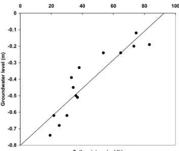
Fig. 1. Relationship between soil moisture (measured with TDR)
and groundwater levels at the HP site in July 2002. Observations
of both variables were available for 14 plots (r2=0.823, P >0.001,
n=14).
We catalogued all vascular plant species at the LP site in July 1999 and in July 2002 at the HP site. Soil sampling was conducted in 2002 and 2003 at the HP and LP sites, respec-tively. Cores of 2.5 (LP) and 5 (HP) cm diameter and up to 30 cm long were collected for soil pH measurement from the O-horizons at eight evenly distributed locations within 2 m of the plot centre. The eight soil samples were bulked to one single sample, air-dried, and analysed for soil pH (H2O, 1:25, soil:solution mass ratio).
Polyethylene tubes with an inner diameter of 9 mm were installed to a depth of 0.7 m as close as possible to the
cen-tre of the plots to measure ground water levels. At one
plot in each study site, the presence of bedrock and boul-ders made it impossible to insert a tube. For the same reason not all tubes were inserted to 0.7 m. We excluded all plots at which groundwater levels were never recorded (38 plots in the LP site and 10 plots in the HP site). Groundwater levels were measured four times (once a month) between June and September 2001 at the LP site and twice during 2002 (July and October) at the HP site. We used the mean of the four groundwater level measurements at the LP site for the sta-tistical analysis. Since summer and fall 2002 were dry, with groundwater levels below 0.7 m in many HP plots, we used only one occasion (October) of groundwater level measure-ments. For the wells for which groundwater levels could be observed in both months the levels were clearly correlated (r=0.69).
At the HP site, soil moisture in the upper 15 cm was measured with a Time Domain Reflectometry (TDR) instru-ment (TRIME FM3 manufactured by IMKO, Germany). The factory-set calibration curve that translates the dielectric
con-stant of the soil into soil water content was used for all mea-surements. The soil water content of a plot was calculated as the mean value of the eight measurements, which were taken at about 2 m distance from the center towards all car-dinal and diagonal directions. At soil water contents above
∼50%, the measurements became unreliable and unrealistic
soil water contents of up to 80–100% were returned for wet soils. While these values obviously are not correct, it was assumed that they still could be used as a relative measure to compare the wetness in the different plots. Very wet plots, in which the ground water was at or close to the ground sur-face and where the TDR measurements gave values of 100% for most points, were excluded from further soil moisture analyses. TDR measurements were performed in July and October 2002. Both measurements were highly correlated (r=0.90) and only the July measurements were used in this paper. Soil moisture and groundwater levels were measured for all plots during a 2–3 day period without precipitation so that the conditions could be assumed to be constant during the measurement period.
For the HP site, the July groundwater and soil moisture measurements were combined into a parameter called “de-gree of wetness”, which allowed ranking of all locations according to soil moisture and groundwater observations. This was motivated by the fact that groundwater observa-tions were not available for dry locaobserva-tions where the levels were more than 0.7 m below the surface; whereas the TDR measured soil moisture was unreliable for wet locations. The “degree of wetness” is an approach to combine soil moisture and groundwater data into one data series. In this way the two methods complemented each other and allowed rank-ing of all plots accordrank-ing to a srank-ingle wetness variable. We performed a linear least square regression with groundwater level as the dependent variable and soil moisture as the pre-dictor. Groundwater level could then be expressed as a func-tion of soil moisture (Fig. 1). For plots (n=22) where only soil moisture content was measured in July a value based on this function was estimated. If only groundwater level was measured there was no modification (n=11). If both TDR and groundwater level were measured, the average of esti-mated and measured groundwater level was used (n=14), i.e., both types of hydrological data were represented and got the same weight. If neither moisture nor ground water level was measured, the location was excluded from the analysis (n=9). The degree of wetness computed in this way was then used to rank the plots according to wetness conditions and these ranks were used for the calculation of Spearman’s rank cor-relations. While the relationship between soil moisture and groundwater is not linear we suppose that a linear approxi-mation is acceptable within the ranges of our measurements for the ranking as described above.
The different variables obviously were correlated to some degree. The correlation coefficients varied from 0.28 to 0.87 (Table 1). With a weak correlation it is possible that dif-ferent methods provide best results, although even with low
correlations one single method could be best in all cases. In general, the correlation matrix suggests two groups of vari-ables. Correlations between plant species richness and soil pH as well as groundwater levels and soil moisture were higher than correlations across these two groups of variables.
2.3 Data analysis
All correlation coefficients between the 2688 different TWI values and the measured variables (plant species richness, soil pH, groundwater level, soil moisture, and wetness de-gree (for the HP site)) for each site were calculated using Spearman’s rank correlation. The results were examined in three ways:
(1) The highest correlation coefficient (HC) between each measured variable and each of the parameter values was identified. For each measured variable this was done by keeping one parameter fixed to a certain value but allowing the other parameters to vary. The variability of the HC within a parameter was then analysed.
(2) The 10% methods (best-10%) resulting in the high-est correlations between TWI and measured variables were selected and distribution functions were compiled for each parameter. We also computed the overlap of the best-10% sets between the two study sites as well as for the different measured variables within each study site. The overlap was computed as the ratio between the number of methods found in both best-10% sets and the total number of methods in a best-10% set (269).
(3) Finally, we determined which calculation methods were most suitable for more than one variable. For each set of correlations between each measured variable and param-eter value the differences (1C) between the highest correla-tion coefficient and all the other correlacorrela-tion coefficients were computed. The measured variables were divided into dif-ferent groups and the mean differences 1C for all variables within a group were calculated. The calculation method with the lowest 1C was considered the most suitable TWI calcu-lation method for this particular group of measured variables. The groups used in this analysis were: (i) all variables from both sites (to obtain an overall best calculation method), (ii) all parameters from the HP site, (iii) all variables from the LP site, (iv) different groups of the measured variables.
The first approach showed the best calculation method for each single measured variable alone, whereas the second ap-proach provided information on how likely a good correla-tion was depending on a certain value for one single param-eter. The two approaches, HC and best-10%, were used to-gether to decide on the best methods for each measured vari-able and were expected to return similar results. The third approach gave a general perception of the processes influ-encing the groups of measured parameters.
29 0.4 0.5 0.6 0.7 0.8 0.9 0 0.2 0.4 0.6 0.8 1
Proportion of tested calculation methods
r HP Species richness HP Soil pH HP GW level LP Species richness LP Soil pH LP GW level
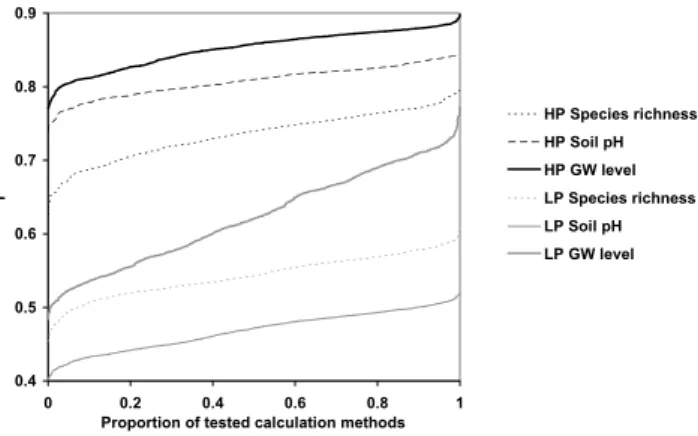
Fig. 2. Accumulated distributions of Spearman rank correlation
co-efficients, increasing from the poorest correlation (left side) to the best correlations (right side), obtained by using the 2688 different TWI values.
3 Results
The correlations between TWI values and measured vari-ables varied considerably between the different calculation methods. The Spearman rank correlation between TWI and soil pH, for instance, varied between 0.40 and 0.52 for the LP site and between 0.74 and 0.84 for the HP site (Fig. 2). Among all variables at both sites the least accurate method gave correlations between 0.11 and 0.29 units lower than the best of the tested methods.
3.1 Single measured variables
Different calculation methods yielded the strongest correla-tions for the different single measured variables at the two study sites. Below we summarize the results for each param-eter (see also Fig. 3 and Table 2).
3.1.1 Flow distribution
The modification of Tarboton’s approach was superior for calculation of flow distribution (Table 2), except for pH and groundwater level at the HP site, where Quinn’s method achieved a higher portion among the best-10% methods.
3.1.2 h exponent
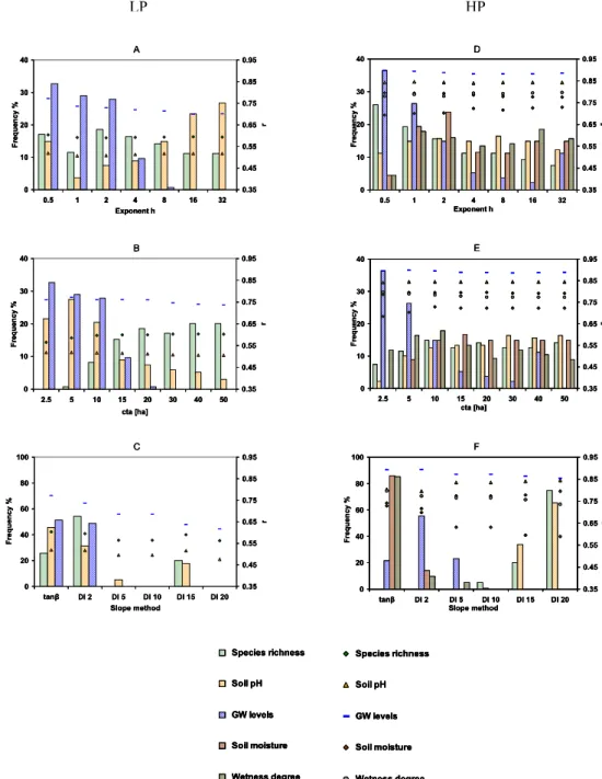
The h values of the best methods were evenly distributed for species richness for the LP site. For pH, higher h values dominated the best-10%, while lower hvalues gave better re-sults for groundwater. The best of the highest correlations (HCs) for species richness and soil pH were similar among all parameter values, whereas the best HC for groundwater was with low h values (Fig. 3a). A slightly different pat-tern was observed at the HP site. For plant species richness and groundwater level, h=0.5 had the best-10% (Fig. 3d). A low h (h=2) also performed best for soil moisture. For
106 R. Sørensen et al.: Evaluation of TWI calculation, based on field observations
Table 1. Pearson correlation coefficients, r, among the measured
variables for the HP-site (Table 1a) and for the LP-site (Table 1b). 1a.
HP – K¨alarna Spec pH GW TDR Wetness
rich level degree
Spec rich 1 pH 0.87 1 GW level 0.48 0.66 1 TDR 0.41 0.61 0.86 1 Wetness degree 0.62 0.78 0.96 0.95 1 1b. LP – ˚Amsele Spec pH GW rich level Spec rich 1 pH 0.62 1 GW level 0.32 0.28 1
soil pH and wetness degree the h=8 and 16, respectively, had slightly better best-10%. The best HCs were found using the three lowest h-exponent values (h=0.5, 1, or 2) for plant species richness, soil pH, and groundwater level while the highest value (h=32) gave the highest HCs for soil moisture and wetness degree (Fig. 3d).
3.1.3 cta
At the LP site, high cta values had the highest portion of the best-10% for species richness, whereas for pH and groundwater level, lower cta values had the highest portion (Fig. 3b). This also applied for the HCs. For the HP site, the groundwater level followed the same pattern, but for the rest of the measured variables the best-10% were evenly dis-tributed and the HCs were similar (Fig. 3e).
3.1.4 cta-down
The decision as to whether or not the area corresponding to cta was routed downslope as groundwater flow did not influ-ence the correlations. In both sites the portion of the best-10% was equally distributed between the two options (not shown).
3.1.5 Slope
For the LP site, tanβ or tanα2 had the largest portion of
the best-10% for species richness, soil pH, and groundwa-ter level (Fig. 3c). The highest HC was found when using tanβ for all three measured variables. At the HP site tanα20
gave best results both with respect to best-10% and HC for soil pH and species richness (Fig. 3f). According to the
best-10% and HC, tanα2 was found to be best for groundwater,
whereas tanβ was best for soil moisture and wetness degree.
3.1.6 Slope-distance
The downslope index computed with the beeline distance performed best for both plant species richness and soil pH at both sites (Table 2). In contrast, the distance following the flow path gave best results for the groundwater levels at both sites and soil moisture at the HP site (Table 2). The slope distance method did not affect the correlations with wetness degree at the HP site.
The large variation in best parameter values for the differ-ent measured variables indicates that there is no single best method. In general, there was also a relatively small over-lap between the best-10% methods for the different mea-sured variables and study sites (Table 3). At the HP site, there was significant overlap between the best methods for plant species number and soil pH as well as among the hy-drological variables (although one has to consider that wet-ness degree was calculated from groundwater level and mois-ture). No overlap at all between any of the hydrological vari-ables and species richness or soil pH was found at the HP site. There was significant overlap at the LP site among all three parameters (Table 3). There was overlap among the hy-drological parameters and between the pH-methods for both sites together. There was also significant overlap between the pH at the HP site and the species richness and the pH at the LP site, but not between the species richness at both sites. However the species richness at the LP site overlapped with the soil moisture at the HP site.
3.2 Grouped measured variables
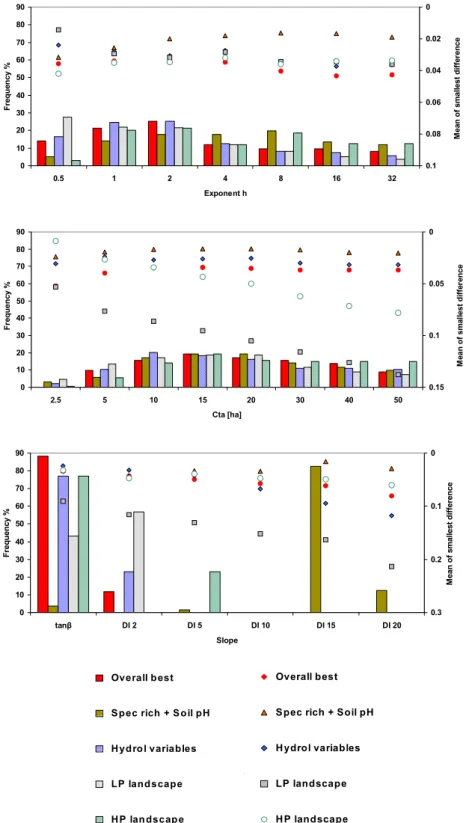
The overall best calculation method, evaluated by the portion among the best-10%, was found when using the modification of Tarboton’s flow distribution, low values of h (h=1–2), the tanβ slope, and cta values of 15 ha. Slope distance did not have any influence on the correlations (Fig. 4, Table 4), nor did the cta-down (not shown).
We identified two groups of measured variables that each had generally similar best-10% distributions, with plant species richness and soil pH in one group, and groundwater level, soil moisture, and wetness degree in the other. The cal-culation parameters performing best for the first group were
Quinn’s flow distribution method, h value of 2–8, tanα15
slope and beeline slope distance, and cta values of 15–20 ha (Fig. 4, Table 4). For the group of hydrological variables, the best results were obtained with Tarboton’s flow distribution,
hvalue of 1–2, cta value of 10–20 ha, tanβ slope, and flow
path slope distance (Fig. 4, Table 4). The parameter cta-down did not have any influence on the correlations (not shown).
Grouping the variables by study site resulted in best per-formance for Tarboton’s flow distribution and tanβ slope for all measured variables in the HP site. The other parameters
30 LP HP 0 10 20 30 40 0.5 1 2 4 8 16 32 Exponent h Fr eq ue n cy % 0.35 0.45 0.55 0.65 0.75 0.85 0.95 r 0 10 20 30 40 2.5 5 10 15 20 30 40 50 cta [ha] Fr eq ue n cy % 0.35 0.45 0.55 0.65 0.75 0.85 0.95 r 0 20 40 60 80 100 tanβ DI 2 DI 5 DI 10 DI 15 DI 20 Slope method Fr equ e ncy % 0.35 0.45 0.55 0.65 0.75 0.85 0.95 r 0 10 20 30 40 0.5 1 2 4 8 16 32 Exponent h Fre q uen cy % 0.35 0.45 0.55 0.65 0.75 0.85 0.95 r 0 10 20 30 40 2.5 5 10 15 20 30 40 50 cta [ha] Frequency % 0.35 0.45 0.55 0.65 0.75 0.85 0.95 r 0 20 40 60 80 100 tanβ DI 2 DI 5 DI 10 DI 15 DI 20 Slope method Fre quenc y % 0.35 0.45 0.55 0.65 0.75 0.85 0.95 r B A C F E D Species richness Soil pH GW levels Soil moisture Wetness degree 0 10 0 2 ct a [ ha] Species richness Soil pH GW levels Soil moisture Wetness degree 0 10 20 30 40 0.5 1 2 4 8 16 32 Exponent h Fr eq ue n cy % 0.35 0.45 0.55 0.65 0.75 0.85 0.95 r 0 10 20 30 40 2.5 5 10 15 20 30 40 50 cta [ha] Fr eq ue n cy % 0.35 0.45 0.55 0.65 0.75 0.85 0.95 r 0 20 40 60 80 100 tanβ DI 2 DI 5 DI 10 DI 15 DI 20 Slope method Fr equ e ncy % 0.35 0.45 0.55 0.65 0.75 0.85 0.95 r 0 10 20 30 40 0.5 1 2 4 8 16 32 Exponent h Fre q uen cy % 0.35 0.45 0.55 0.65 0.75 0.85 0.95 r 0 10 20 30 40 2.5 5 10 15 20 30 40 50 cta [ha] Frequency % 0.35 0.45 0.55 0.65 0.75 0.85 0.95 r 0 20 40 60 80 100 tanβ DI 2 DI 5 DI 10 DI 15 DI 20 Slope method Fre quenc y % 0.35 0.45 0.55 0.65 0.75 0.85 0.95 r B A C F E D 0 10 20 30 40 0.5 1 2 4 8 16 32 Exponent h Fr eq ue n cy % 0.35 0.45 0.55 0.65 0.75 0.85 0.95 r 0 10 20 30 40 2.5 5 10 15 20 30 40 50 cta [ha] Fr eq ue n cy % 0.35 0.45 0.55 0.65 0.75 0.85 0.95 r 0 20 40 60 80 100 tanβ DI 2 DI 5 DI 10 DI 15 DI 20 Slope method Fr equ e ncy % 0.35 0.45 0.55 0.65 0.75 0.85 0.95 r 0 10 20 30 40 0.5 1 2 4 8 16 32 Exponent h Fre q uen cy % 0.35 0.45 0.55 0.65 0.75 0.85 0.95 r 0 10 20 30 40 2.5 5 10 15 20 30 40 50 cta [ha] Frequency % 0.35 0.45 0.55 0.65 0.75 0.85 0.95 r 0 20 40 60 80 100 tanβ DI 2 DI 5 DI 10 DI 15 DI 20 Slope method Fre quenc y % 0.35 0.45 0.55 0.65 0.75 0.85 0.95 r B A C F E D Species richness Soil pH GW levels Soil moisture Wetness degree 0 10 0 2 ct a [ ha] Species richness Soil pH GW levels Soil moisture Wetness degree Species richness Soil pH GW levels Soil moisture Wetness degree 0 10 0 2 ct a [ ha] Species richness Soil pH GW levels Soil moisture Wetness degree Species richness Soil pH GW levels Soil moisture Wetness degree 0 10 0 2 ct a [ ha] Species richness Soil pH GW levels Soil moisture Wetness degree
Fig. 3. Distributions for each measured variable of the best 10% calculation methods (bars) among different values of the exponent h,
the slope method (including different values for the d in the downslope index), and the creek initiation area, cta. The highest correlation coefficients (HC) obtained using a certain parameter value are shown by symbols. The figures (a–f) show the distributions for the three different parameters in the two study areas: (a) h in the LP site. (b) cta in the LP site. (c) slope in the LP site. (d) h in the HP site. (e) cta in the HP site. (f) slope in the HP site. Note the different scale on the y-axis for the slope method.
exhibited no significant influence on correlations for this site, but h values of 0.5 and cta values of 2.5–5 gave lower cor-relations (Fig. 4, Table 4). In the LP site Tarboton’s flow distribution, low values of h (0.5–2), cta values of 10–20, tanαd2 slope, and the beeline distance yielded the best
re-sults (Fig. 4, Table 4). Cta-down did not have any effect on the results in any of the sites (not shown).
The best calculation methods when grouping the measured variables according to type or site resulted in correlation co-efficients between the overall best calculation method and the best calculation method for each single measured variable (Table 5).
108 R. Sørensen et al.: Evaluation of TWI calculation, based on field observations
31
Figure 4
0 10 20 30 40 50 60 70 80 90 0.5 1 2 4 8 16 32 Exponent h Fr eque nc y % 0 0.02 0.04 0.06 0.08 0.1 M ea n o f sma lles t d if fe re nc e 0 10 20 30 40 50 60 70 80 90 2.5 5 10 15 20 30 40 50 Cta [ha] Fr eq ue nc y % 0 0.05 0.1 0.15 M ean o f sm al le st d if fe re nce 0 10 20 30 40 50 60 70 80 90 tanβ DI 2 DI 5 DI 10 DI 15 DI 20 Slope Fr eq ue nc y % 0 0.1 0.2 0.3 M ean o f sm al le st d if fe re n ce -10 10 30 50 70 90 Overall best Spec rich + Soil pH Hydrol variables LP landscape HP landscape -10 10 30 50 70 90 0 2 Overall best Spec rich + Soil pH Hydrol variables LP landscape HP landscape 0 10 20 30 40 50 60 70 80 90 0.5 1 2 4 8 16 32 Exponent h Fr eque nc y % 0 0.02 0.04 0.06 0.08 0.1 M ea n o f sma lles t d if fe re nc e 0 10 20 30 40 50 60 70 80 90 2.5 5 10 15 20 30 40 50 Cta [ha] Fr eq ue nc y % 0 0.05 0.1 0.15 M ean o f sm al le st d if fe re nce 0 10 20 30 40 50 60 70 80 90 tanβ DI 2 DI 5 DI 10 DI 15 DI 20 Slope Fr eq ue nc y % 0 0.1 0.2 0.3 M ean o f sm al le st d if fe re n ce -10 10 30 50 70 90 Overall best Spec rich + Soil pH Hydrol variables LP landscape HP landscape -10 10 30 50 70 90 0 2 Overall best Spec rich + Soil pH Hydrol variables LP landscape HP landscapeFig. 4. Distribution of the best 10% calculation methods (bars) among different values of the exponent h, the slope method (including different
values for the d in the downslope index), and the creek initiation area, cta, for different groups of measured variables. The symbols show how much correlation coefficients decrease when using the best method for a group instead of the best method for the individual variables. This was expressed as the mean of the differences between the highest correlation coefficients obtained for each individual variable and the highest correlation coefficients, which were obtained for the entire group for a certain parameter value.
Table 2. Distribution of the best 10% of all tested calculation methods (using different measured variables) for flow distribution and slope
distance respectively. Note that there were only two options for each of these two parameters. As both options were tested equally often in all cases, the deviation from a 50-50 distribution indicates how important a certain choice is. The highest Spearman’s rank correlation
coefficients, rs, which were obtained with a certain method, are given in brackets.
LP site ( ˚Amsele) HP site (K¨alarne)
Flow distribution method Species pH Ground-water Species pH Ground-water Soil Wetness
richness richness moisture degree
Tarboton 63 60 59 55 33 41 78 68
(0.604) (0.519) (0.762) (0.795) (0.842) (0.894) (0.729) (0.797)
Quinn 37 40 41 45 67 59 22 32
(0.590) (0.515) (0.772) (0.793) (0.845) (0.898) (0.700) (0.787)
Slope distance method (for tanαd)
Beeline 79 76 40 100 100 13 41 49
(0.604) (0.519) (0.760) (0.795) (0.845) (0.892) (0.729) (0.797)
Along flow path 21 24 60 0 0 87 59 51
(0.589) (0.510) (0.772) (0.771) (0.829) (0.898) (0.729) (0.797)
Table 3. Overlapping between the best 10% calculation methods for the different measured variables. The overlap was computed as the ratio
between the number of methods found in both best-10% sets (of the measured variables to be compared) and the total number of methods in a best-10% set (n=269). For random drawings the overlapping ratio would be smaller than 0.071 with a probability of 0.05 and higher than 0.127 with a probability of 0.95.
LP site ( ˚Amsele) HP site (K¨alarne)
Species pH Ground-water Species pH Ground-water Soil Wetness
richness richness moisture degree
Species richness 1 0.290 0.320 0 0.186 0.119 0.215 0.082
LP site ( ˚Amsele) pH 1 0.142 0.007 0.142 0.052 0.126 0.261
Groundwater 1 0 0 0.424 0.379 0.254
Species richness 1 0.677 0 0 0
pH 1 0 0 0
HP site (K¨alarne) Groundwater 1 0.163 0.178
Soil moisture 1 0.751
Wetness degree 1
4 Discussion
Our results demonstrate that different methods of calculat-ing the TWI indeed produce a high variation in correlation strengths between the various TWI values and the different measured variables. There was not one single method that was optimal for all variables and study sites. Overall, the overlap of the best-10% between either measured variables or study sites was rather small (Table 3). However, general characteristics for methods yielding the best-10% could be observed for certain groups of variables.
The correlation coefficients decreased with the general-ity of the calculation method. The best overall calculation method did not yield as strong correlations as the best
calcu-lation methods for each single measured variable. However, the latter calculation methods were only optimal for a par-ticular variable and study site and are thus of more limited general applicability.
In our study, the modification of Tarboton’s flow distribu-tion method was in general superior to Quinn’s distribudistribu-tion method. This was expected, since Quinn’s method tends to overestimate flow dispersion and braiding, especially in near-stream areas (Kim and Lee, 2004). Pan et al. (2004) found the multiple flow direction to be geometrically more accurate than the single flow direction algorithm in idealized DEMs. Our empirical study also found that the multiple directional flow algorithms were superior to the single-directional algo-rithm in both Quinn’s and Tarboton’s methods. However,
110 R. Sørensen et al.: Evaluation of TWI calculation, based on field observations
Table 4. Distribution of the best 10% of all tested calculation methods (using different groups of measured variables) for flow distribution
and slope distance respectively. Note that there were only two options for each of these two parameters. As both options were tested equally often in all cases, the deviation from a 50-50 distribution indicates how important a certain choice is. The mean of the difference between the very best correlation coefficient for each measured parameter and the group wise best correlation coefficient are given in brackets.
Species Groundwater, LP HP All
richness soil moisture ( ˚Amsele) (K¨alarne)
and pH and wetness site site
degree Flow distribution method
Tarboton 41 71 87 74 77
(0.093) (0.181) (0.154) (0.114) (0.125)
Quinn 59 29 13 26 23
(0.096) (0.168) (0.152) (0.112) (0.123)
Slope distance method (for tanαd)
Beeline 91 37 58 52 48
(0.084) (0.181) (0.154) (0.104) (0.121)
Along flow path 9 63 42 48 52
(0.096) (0.169) (0.149) (0.114) (0.125)
Table 5. Best Spearman rank correlation coefficients obtained for the single measured variables at each site and for different groups of
variables. Correlation coefficients for correlations where the particular variable is included in the respective group are in bold. Best correlation for groups of variables
Best possible Species richness Groundwater, soil LP site HP site All
correlation for and pH moisture and ( ˚Amsele) (K¨alarne)
each variable wetness degree
LP site ( ˚Amsele) Species richness 0.604 0.587 0.556 0.597 0.570 0.580 pH 0.519 0.505 0.492 0.513 0.497 0.498 Groundwater 0.772 0.582 0.772 0.743 0.711 0.722 HP site (K¨alarne) Species richness 0.795 0.765 0.667 0.716 0.730 0.739 pH 0.845 0.840 0.757 0.795 0.798 0.802 Groundwater 0.898 0.835 0.886 0.872 0.862 0.871 Soil moisture 0.729 0.582 0.676 0.674 0.723 0.702 Wetness degree 0.797 0.721 0.765 0.746 0.792 0.772
optimal values for h were larger than one in some cases, in-dicating that the usual multidirectional flow algorithm might sometimes result in too large a spreading of the accumulated area. Holmgren (1994b) suggests a value of h between 4 and 6 irrespective of DEM resolution. In our study the best corre-lations for the hydrological variables were mainly found with lower values of h (0.5–2). The value of h could depend on the steepness in the studied landscape. Our results combined with those of G¨untner et al. (2004), who found h values of 8– 10 to be most suitable in a mountainous catchment, suggest that h might decrease when going from mountainous (with steeper slopes) to hilly areas.
The best-10% differed in terms of slope calculation
be-tween the two groups of measured variables. For plant
species richness and soil pH, a higher slope distance (tanαd15)and the beeline distance should be used, while for
the hydrological variables best results were obtained with tanβ slope and slope distance calculated along the flow path. The difference in d indicates that downslope drainage con-ditions are more important for the plant species richness and soil pH than for groundwater level, soil moisture, and wet-ness degree. A possible explanation is that local slope in-fluences the hydrological variables, while larger geomorpho-logic features are more important for species richness of vas-cular plants and soil pH. For example, a site on a plateau with relatively small upstream area but a low slope can be quite moist but have low soil pH and plant species richness. A higher value of d gives information about the downslope
conditions, which can indicate where along a slope the site is situated. A gentle slope would be found in the lower parts of a hill, while a steeper slope would indicate that the point is situated in a recharge area. Groundwater recharge and dis-charge areas differ considerably in terms of soil pH and plant species richness, with both increasing towards discharge ar-eas (Giesler et al., 1998; Zinko et al., 2005).
G¨untner et al. (2004) found that a cta of 6–10 ha worked best for the TWI used to predict water-saturated areas. In our study cta values of 10 to 20 ha generally gave the best cor-relations for the measured hydrological variables. However, the cta did not have much influence on the strength of the correlations, which may be because most plots were located in non-creek cells regardless of the value of cta. Although G¨untner et al. (2004) found a smaller value of cta, indicat-ing that creeks start with less accumulated area, precipitation in their study catchment was roughly twice that in our sites. Kim and Lee (2004) found an optimal cta value of 20 ha for estimation of the creek network in their catchment in South Korea.
Correlation coefficients were in general higher at the HP site than at the LP site. This difference might be explained by the fact that the pH range in the HP area is greater than that of the LP area, meaning that there is more variation in pH to be explained by the TWI.
Grouping the variables helped to identify some guiding principles and allow speculating about physical explanations. For instance, higher values for d in the downslope index (i.e., an integration of the slope over a larger scale) gave better re-sults for the correlation with soil pH and species richness, whereas the local slope worked better for soil moisture. One might argue that this could be because soil pH and species richness depend more on long-term lateral flow processes that redistribute weathering products within the catchment. In contrast the soil moisture at the surface reflects current conditions and is more sensitive to local topographical fea-tures.
5 Concluding remarks
This study was a first attempt to find a general calculation method for the TWI that would be valid for the spatial distri-bution of plant species richness, soil pH, groundwater level, and soil moisture in Fennoscandian boreal forest. We were not able to identify one single best method since different methods gave best correlations with the different measured variables. Although not as pronounced as for the different variables the best methods were also site specific. However, “compromise” methods that yielded best calculations for the different measured variables were identified. In general, the modified Tarboton’s flow distribution performed better than Quinn’s method, and a low h value yielded the best results. The local slope tanß was found in most cases to be superior to the use of the tanαd slope. However, a higher d value and
the beeline slope distance were best for estimating soil pH and species richness, while tanβ and flow path slope distance were best for estimating the hydrological variables.
It might be useful to explore, if at least some data are avail-able, the variety of calculation methods for the topographical index prior to performing estimates based on it. Our results also indicate the need to further refine the algorithms. Some calculation parameters could be variable in time or space. The value of cta, for instance, could vary with slope or sea-son and the value of h could vary with soil type or slope. The species richness of vascular plants and the pH, however, are not expected to vary seasonally.
Acknowledgements. We thank K. Holmstr¨om, Metria, for the
interpretation of aerial photographs, and J. Temnerud, J. Lindeberg, ˚
A. Laurell, T. G¨othner, L. Ahnby, M. Juutilainen, G. Nordenmark, G. Nilsson, P.-E. Wikberg, G. Brorsson, J. Englund, M. Larsson, E. Carlborg, M. Svedmark and C. Reidy for fieldwork assistance. We also thank N. Hjerdt and K. Bishop for valuable comments, and K. McGlynn for copy editing. Funding for this project was provided by the Swedish Research Council (R. Sørensen and J. Seibert) as well as by the Lamm Foundation, the Foundation for Strategic Environmental Research (MISTRA), the Swedish Research Council for Environment, Agricultural Sciences and Spatial Planning, the Swedish Research Council, J.C. Kempes Minnes Foundation, and Gunnar and Birgitta Nordin’s Foundation (UZ).
Edited by: L. Pfister
References
Band, L. E., Patterson, P., Nemani, R., and Running, S. W.: Forest ecosystem processes at the watershed scale: incorporating hills-lope scale, Agr. Forest Meteorol., 63, 93–126, 1993.
Beven, K. J. and Kirkby, M. J.: A physically based, variable con-tributing area model of basin hydrology, Hydrolological Sciences Bulletin, 24, 43–69, 1979.
Beven, K. J., Wood, E. F., and Sivapalan, M.: On hydrological het-erogeneity – catchment morphology and catchment response, J. Hydrol., 100, 353–375, 1988.
Burt, T. and Butcher, D.: Stimulation from simulation – a teach-ing model of hillslope hydrology for use on microcomputers, J. Geogr. Higher Educ., 10, 23–39, 1986.
Famiglietti, J. S. and Wood, E. F.: Evapotranspiration and runoff from large land areas – land surface hydrology for atmospheric general-circulation models, Surv. Geophys., 12, 179–204, 1991. Florinsky, I. V., McMahon, S., and Burton, D. L.: Topographic con-trol of soil microbial activity: a case study of denitrifiers, Geo-derma, 119, 33–53, 2004.
Giesler, R., H¨ogberg, M., and H¨ogberg, P.: Soil chemistry and plants in Fennoscandian boreal forest as exemplified by a local gradient, Ecology, 79, 119–137, 1998.
Gough, L., Shaver, G. R., Carroll, J., Royer, D. L., and Laundre, J. A.: Vascular plant species richness in Alaskan arctic tundra: the importance of soil pH, J. Ecol., 88, 54–66, 2000.
112 R. Sørensen et al.: Evaluation of TWI calculation, based on field observations Grayson, R. B., Bl¨oschl, G., Western, A. W., and McMahon, T. A.:
Advances in the use of observed spatial patterns of catchment hy-drological response, Adv. Water Resour., 25, 1313–1334, 2002. Grubb, P. J.: Global trends in species-richness in terrestrial
vege-tation: a view from the northern hemisphere, in: Organization of Communities Past and Present, edited by: Gee, J. H. R. and Giller, P. S., Blackwell, pp. 98–118, 1987.
G¨untner, A., Seibert, J., and Uhlenbrook, S.: Modeling spatial pat-terns of saturated areas: an evaluation of different terrain indices, Water Resour. Res., 40, W05114, doi:10.1029/2003WR002864, 2004.
Hjerdt, K. N., McDonnell, J. J., Seibert, J., and Rodhe,
A.: A new topographic index to quantify downslope
con-trols on local drainage, Water Resour. Res., 40, W05602, doi:10.1029/2004WR003130, 2004.
H¨ogberg, P., Johannisson, C., Nicklasson, H., and H¨ogbom, L.: Shoot nitrate reductase activities of field-layer species in differ-ent forest types, Scand. J. Forest Res., 5, 449–456, 1990. Holmgren, P.: Topographic and geochemical influence on the forest
site quality, with respect to Pinus sylvestris and Picea abies in Sweden, Scand. J. Forest Res., 9, 75–82, 1994a.
Holmgren, P.: Multiple flow direction algorithms for runoff mod-elling in grid based elevation models: an empirical evaluation, Hydrol. Process., 8, 327–334, 1994b.
Kim, S. and Lee, H.: A digital elevation analysis: a spatially distributed flow apportioning algorithm, Hydrol. Process., 18, 1777–1794, 2004.
Moore, I. D., Grayson, R. B., and Ladson, A. R.: Digital terrain modeling – a review of hydrological, geomorphological, and bi-ological applications, Hydrol. Process., 5, 3–30, 1991.
Moore, I. D., Norton, T. W., and Williams, J. E.: Modelling envi-ronmental heterogeneity in forested landscapes, J. Hydrol., 150, 717–747, 1993.
Pan, F., Peters-Lidard, C. D., Sale, M. J., and King, A. W.: A com-parison of geographical information system-based algorithms for computing the TOPMODEL topographic index, Water Resour. Res., 40, 1–11, 2004.
P¨artel, M.: Local plant diversity patterns and evolutionary history at the regional scale, Ecology, 83, 2361–2366, 2002.
Quinn, P., Beven, K., Chevallier, P., and Planchon, O.: The predic-tion of hillslope flow paths for distributed hydrological modeling using digital terrain models, Hydrol. Process., 5, 59–79, 1991. Quinn, P. F., Beven, K. J., and Lamb, R.: The ln(a/tan beta) index:
how to calculate it and how to use it within the TOPMODEL framework, Hydrol. Process., 9, 161–182, 1995.
Raab, B. and Vedin, H.: The national atlas of Sweden: climate, lakes and rivers, SNA Publisher, Stockholm, 1995.
Robson, A., Beven, K., and Neal, C.: Towards identifying sources of subsurface flow: a comparison of components identified by a physically based runoff model and those determined by chemical mixing techniques, Hydrol. Process., 6, 199–214, 1992. Rodhe, A. and Seibert, J.: Wetland occurrence in relation to
topog-raphy: a test of topographic indices as moisture indicators, Agr. Forest Meteorol., 98–99, 325–340, 1999.
Sariyildiz, T., Anderson, J. M., and Kucuk, M.: Effects of tree species and topography on soil chemistry, litter quality, and de-composition in Northeast Turkey, Soil Biol. Biochem., 37, 1695– 1706, 2005.
Seibert, J., Bishop, K. H., and Nyberg, L.: A test of TOPMODEL’s ability to predict spatially distributed groundwater levels, Hy-drol. Process., 11, 1131–1144, 1997.
Sivapalan, M. and Wood, E. F.: A multidimensional model of non-stationary space-time rainfall at the catchment scale, Water Re-sour. Res., 23, 1289–1299, 1987.
Sivapalan, M., Wood, E. F., and Beven, K. J.: On hydrologic sim-ilarity. 3. A dimensionless flood frequency model using a gen-eralized geomorphologic unit hydrograph and partial area runoff generation, Water Resour. Res., 26, 43–58, 1990.
Tarboton, D. G.: A new method for the determination of flow direc-tions and upslope areas in grid digital elevation models, Water Resour. Res., 33, 309–319, 1997.
Whelan, M. J. and Gandolfi, C.: Modelling of spatial controls on denitrification at the landscape scale, Hydrol. Process., 16, 1437– 1450, 2002.
White, J. D. and Running, S. W.: Testing scale-dependent assump-tions in regional ecosystem simulaassump-tions, J. Veg. Sci., 5, 687–702, 1994.
Wolock, D. M. and McCabe, G. J.: Comparison of single and multi-ple flow direction algorithms for computing topographic param-eters in Topmodel, Water Resour. Res., 31, 1315–1324, 1995. Zinko, U., Seibert, J., Dynesius, M., and Nilsson, C.: Plant species
numbers predicted by a topography based groundwater-flow in-dex, Ecosystems, 8, 430–441, 2005.
Zinko, U.: Plants go with the flow – predicting spatial distribution of plant species in the boreal forest, ISBN 91-7305-705-3, PhD thesis, Ume˚a University, Department of Ecology and Environ-mental Science, 2004.