Predicting the effects of changes in thermal envelope characteristics on energy consumption : application and verification of a simple model for Australian and Canadian climates

Publisher’s version / Version de l'éditeur:

Energy and Environment, 7, 1, pp. 1-28, 1996

READ THESE TERMS AND CONDITIONS CAREFULLY BEFORE USING THIS WEBSITE. https://nrc-publications.canada.ca/eng/copyright

Vous avez des questions? Nous pouvons vous aider. Pour communiquer directement avec un auteur, consultez la première page de la revue dans laquelle son article a été publié afin de trouver ses coordonnées. Si vous n’arrivez pas à les repérer, communiquez avec nous à PublicationsArchive-ArchivesPublications@nrc-cnrc.gc.ca.

Questions? Contact the NRC Publications Archive team at

PublicationsArchive-ArchivesPublications@nrc-cnrc.gc.ca. If you wish to email the authors directly, please see the first page of the publication for their contact information.

NRC Publications Archive

Archives des publications du CNRC

This publication could be one of several versions: author’s original, accepted manuscript or the publisher’s version. / La version de cette publication peut être l’une des suivantes : la version prépublication de l’auteur, la version acceptée du manuscrit ou la version de l’éditeur.

Access and use of this website and the material on it are subject to the Terms and Conditions set forth at

Predicting the effects of changes in thermal envelope characteristics

on energy consumption : application and verification of a simple model

for Australian and Canadian climates

Cornick, S. M.; Thomas, P. C.; Prasad, D. K.

https://publications-cnrc.canada.ca/fra/droits

L’accès à ce site Web et l’utilisation de son contenu sont assujettis aux conditions présentées dans le site

LISEZ CES CONDITIONS ATTENTIVEMENT AVANT D’UTILISER CE SITE WEB.

NRC Publications Record / Notice d'Archives des publications de CNRC:

https://nrc-publications.canada.ca/eng/view/object/?id=9c8dca0d-3e64-4d27-a4be-8f5f25d6e356 https://publications-cnrc.canada.ca/fra/voir/objet/?id=9c8dca0d-3e64-4d27-a4be-8f5f25d6e356

Predicting the Effects of Changes in Thermal Envelope

Characteristics in Energy Consumption: Application and Verification

of a Simple Model for Australian and Canadian Climates

by

S.M. Cornick, P.c. Thomas and D.K. Prased

Reprinted from

ENERGY

&

ENVIRONMENT

VOLUME 7 No.1 1996

MULTI-SCIENCE PUBLISHING CO. LTD.

Energy& Environment, Vol. 7, 1996, Issue 1

PREDICTING THE EFFECTS OF CHANGES IN

THERMAL ENVELOPE CHARACTERISTICS ON

ENERGY CONSUMPTION:

APPLICATION AND VERIFICATION OF A SIMPLE MODEL

FOR AUSTRALIAN AND CANADIAN CLIMATES

S. M. Cornick!, P.e. Thomas2_{and D.K. Prasad}3

ABSTRACT: A simple energy model was used for determining thermal envelope characteris-tics and building envelope trade-off procedures for the new Canadian and Australian energy efficiency codes for new buildings. The model relates heating and cooling system loads to enve-lope thermal characteristics. It was deveenve-loped from thousands of DOE2.1 E simulation runs. Two separate databases, one containing 25 Canadian locations and the other containing 9 Australian locations were created. The heating and cooling models were developed from these databases. The model is shown to give consistent results although there are significant differ-ences in climate, construction of the building envelope, building operational schedules and HVAC system configurations. This paper briefly describes the DOE2.1 E models used for the study in each country, highlighting similarities and differences. The consistency of results pre-dicted by the model is discllssed for typical climatic locations in both countries. The methods for predicting heating and cooling system loads are shown to produce good results over a wide range of climates and for different system configurations. The paper also discusses the devel-opment of climate correlations to extend the range of the models to include locations not in the original databases.

INTRODUCTION

Canada and Australia are in the process of developing national energy efficiency codes for buildings as part of continuing government initiatives to reduce energy consump-tion and the resulting rate of increase of greenhouse gas emissions. This paper outlines a simple model used to predict energy consumption in perimeter zones (Cornick and Sander, 1995). The performance of the model is compared for various building con-structions, operation schedules, HVAC system configurations, and climates. Specifically, a comparison is made between heating climates (Canada) and cooling cli-mates (Australia). In Canada the developed model forms an integral part of the pre-scriptive and trade-off compliance paths of the National Energy Code for Buildings. In Australia, the model is being reviewed by Standards Australia for use as a systems IResearch Officer, Institute for Research in Construction, National Research Council of Canada, Montreal Road Campus, Ottawa Ontario, Canada. K I A OR6.

2projcct Scicntisl.

'Director, SOLARCH - The National Solar Architecture Research Unit, School of Architecture, The University of New South Walcs, Sydney2052,Australia.

2 Changes in Thermal Envelope Characteristics on Energy Consumption

performance compliance method for building envelopes.

The Canadian Code

In Canada, two separate energy codes were produced; a code for houses and a code for buildings. Part 3 of the code for buildings specifies the thermal characteristics of the building envelope (National Energy Code for Buildings). The envelope portion of the Canadian code has three compliance paths: a prescriptive path, a trade-off path, and a full performance path. The trade-off and full performance procedures use the pre-scriptive requirements to calculate the energy budget of a reference building against which the proposed design is compared.

The prescriptive requirements generated for the Canadian code were based on eco-nomic criteria. The optimal ecoeco-nomic envelope characteristics were determined by minimizing the sum of incremental construction costs and the present value of the energy costs over the life cycle of the envelope (Sanderet aI., 1995). A simple model predicting changes in heating and cooling system loads were required for the life cycle costing procedure. This model was also specified as the energy calculation method for the trade-off compliance path for the Canadian Code (Sander and Cornick, 1994).

The Australian Code

Separate research efforts are being carried out which will culminate in energy effi-ciency standards for both residential and commercial buildings in Australia. The Nationwide Home Energy Rating Scheme (NatHERS) is a simulation based approach for domestic houses, which will lead to star rating of homes based on energy perfor-mance. Two studies have been carried out for commercial buildings. The Commercial Building Energy Code project phase-l (CBEC) study determined cost effective levels of energy efficiency for various components of four building systems (SRCI, 1993). The National Solar Architecture Research Unit at the University of New South Wales (SOLARCH) developed the database and trade-off equations for the building envelope using the parameters and models described in this paper in a study sponsored jointly by the Energy Research and Development Corporation and Standards Australia, (Prasad, 1994). Further research is anticipated to combine and extend the findings of these two studies into a full fledged Commercial Building Energy Code.

For the Australian code, it is envisaged that compliance via the systems perfor-mance option could be a two step process. First, the allowable energy budget for the perimeter zones are computed using the prescriptive values (derived from least life cycle cost considerations under a specified economic scenario) applied to a proposed building design. Trade-offs to the envelope characteristics of the proposed design are then allowed as long as the energy budget is less than or equal to energy budget of the prescriptive case. A simple model was required to quickly calculate the allowable energy budget and energy use of the proposed design. This trade-off procedure is sim-ilar to the trade-off path in the proposed Canadian Code.

PARAMETERS

The most important part of the process in the development of the predictive energy models was the development of a method to characterize and study the effects of

enve-Changes in Thermal Envelope Characteristics on Energy Consumption 3

lope characteristics on energy consumption. A key element of this method was the de-coupling of the relevant envelope characteristics in order to conduct parametric stud-ies on the building envelope. The thermal propertstud-ies of the building envelope were characterized by three parameters. Crawley (1992) provides a detailed explanation as to how these parameters were derived. The three parameters are; V, a transmission parameter which accounted for heat loss or gain through the envelope, V, a solar para-meter which accounted for solar gains through the envelope, and W, an internal gain parameter which characterized internal loads in the perimeter zone, specifically lights, equipment and people. It was decided not to include a parameter for internal mass in the parametric analysis (Crawley, 1992; Crawley, Schliesing, and Boulin 1990). Internal mass can shift the timing and change the magnitude of peak cooling and heat-ing loads. However for most buildheat-ings with typical values ofV, V, and Wand typical operating schedules the effect of mass on total energy use is small (10% or less). Although mass may effect the total annual energy consumption, the slopes represent-ing the change in heatrepresent-ing and coolrepresent-ing system loads for a correspondrepresent-ing change in the parametersV, V, and W do not change significantly with mass (Cornick and Sander, 1995). The ranges of these envelope parameters were chosen to suit local practices and climates thus allowing envelope studies to be conducted for a wide range of climates and construction types. The parameters were defined as:

Dimensionless W/m2

where:

Awall == opaque wall area, m2

Aglass == window wall area including frame, m2 Atotal ==gross wall area, (A w+ Ag), m2

A_noor ==floor area associated with envelope, typically 4.5 m deep (5m for the Australian study), m2

Vwall ==opaque wall V-value, W/m2_-oK

ｖｾｬ｡ｳｳ == window V-value, including frame, W/m2_-oK SCg1ass == window shading coefficient

I == design heat gain from lights, people, and equipment, W/m2_{floor area.}

ASSVMPTIONS

Simple buildings were simulated in order to isolate the three thermal parameters,V,

V, and W from the effect of ground and roof interaction. The building model is a mod-ification of a five zone model used to develop the first set of regression equations for

4 Changes in Thermal Envelope Characteristics on Energy Consumption

ASHRAE Special Project 41 (Pacific Northwest Laboratory 1983) in order to update ASHRAE 90.1. Similar models and methods were used to revise the regression equa-tions in 90.1 (Berkeley Solar Group, 1986; Wilcox, 1991). The California Energy Commission (CEC) used a similar model in setting the requirements for its third gen-eration nonresidential energy standards (CEC 1990). DOE2 was the energy simulation tool used for all of these studies. A recent comparison of DOE2 with other simulation tools as part of the BESTEST program shows that DOE2 gives results comparable to other simulation tools (Judkoff and Neymark, 1995). For the marginal differences used for code calculation purposes the results produced from DOE2 and the perimeter zone model were deemed acceptable. Several building specific and operational assumptions were made to reflect the typical construction practices in both countries. The differ-ences stem mainly from the fact that the Australian climate is cooling dominated while the climate in Canada is heating dominated. For example the maximum value of U for Australia is 3.38 (single glazing) whereas in Canada the maximum practical value of U is 2.839 (double glazing). Operational assumptions also reflect the climate differ-ences. In Australia for example, it is common practice to shut off all HYAC equipment after hours. In Canada however buildings cannot be operated in this mode; heating, usually with thermostat setback, must be available at night.

Canadian NRCC Model

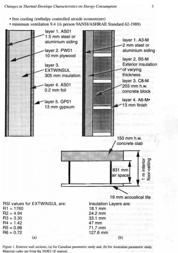
The model simulated for the National Research Council of Canada (NRCC) paramet-ric study was a four zone building. Each zone represented a strip of exterior walliocat-ed at mid height of a typical building and facing one of the cardinal orientations. The central core zone was not modelled. Adiabatic interior walls and floor/ceiling bound each of the perimeter zones. A medium weight floor (340 kg/m2) was chosen to sim-ulate the effect of internal mass. Windows are assumed to be a strip of double glazed window running the entire length of the zone. The exterior wall of a perimeter zone was a five layer wall comprising, an outside finish (2 mm steel siding), 10 mm of ply-wood sheathing, a layer of insulation (305 mm), a layer of foil (0.2 mm), and an inte-rior finish (13 mm of gypsum). The exteinte-rior wall, shown in Figure la, had little mass, about (137 kg/m2).Crawley (1992) provides a detailed specification of the DOE2.1 E model used for Canadian Energy Code.

The fixed assumptions for each zone were: • no interzone heat transfer

• fixed infiltration rate 0.25 l/s/m2

• internal loads on a six day office schedule

• heating setback to 15'C and cooling off when unoccupied

• medium weight floor construction, 200 mm heavy weight concrete slab • light wall construction

System specific assumptions were: • packaged YAY system with terminal reheat • 13°C supply air

Changes in Thermal Envelope Characteristics on Energy Consumption 5 ... C> .Q

....

c::

-Q)= -_c:: Q)_u ' - I E

<5

o

...

;;::: layer 1. A3-M 2 mm steel or aluminium siding layer 2. B5-M Exterior insulation of varying thickness layer 3. C8-M 203 mm h.w. concrete block 150 mm h.w. concrete slab 831 mm air space layer 4. A6-M· ...oQl...-13 mm finish layer 2. PW01 10 mm plywood layer 3. EXTWINSUL 305 mm insulation layer4. AS01 0.2 mm foil layer 5. GP01 13 mm gypsum

• free cooling (enthalpy controlled airside economizer)

• minimum ventilation 9.4 1/s person 9ANSIIASHRAE Standard 62-1989) layer 1. AS01

1.5 mm steel or aluminium siding

RSI values for EXTWINSUL are: R1

=

1760 R2

=

4.94 R3

=

3.30 R4= 1.42 R5

=

0.98 R6=0.72 19 mm acoustical tile Insulation Layers are:

18.1 mm 24.2 mm 33.1 mm 47 mm 71.7 mm 127.6 mm (a) (b)

Figure I. Exterior wall sections, (a) for Canadian parametric study and, (b) for Australian paramelric sludy. Malerial codes are from the DOE2.1 E manual.

6 Changes in Thermal Envelope Characteristics on Energy Consumption

Australian Model

Initially it was planned to use the simulated results of the 12 perimeter zones of a three floor, 15 zone building based around the model used to set the stringency levels in the CBEC study. The basic model is similar to the Canadian model except for the HVAC system and the increased wall mass. The wall section, shown in Figure 1b, was a four layer wall consisting of an exterior finish layer, an insulation layer of varying thick-ness, a single heavy weight concrete block, and an interior finish. The wall mass was about twice the mass of the Canadian model ranging from 225 to 235 kg/m2.The floor weights for both models were similar. Initial runs showed differences in the energy use for the top and ground floors due to roof and floor interactions. Reviewing the project objectives, it was felt that a simple but effective trade-off procedure for the vertical envelope could be developed by using the energy performance of the middle floor perimeter zones only. Therefore only the energy performance for the middle floor were used in deriving the envelope trade-off equations. The final simulation model had the following major differences from that used in the NRCC study.

• a five and half day office schedule

• cooling and heating were not available after office hours (no setback) • fixed infiltration rate 0.25 air changes/hr (0.35 1/s/m2)

• a Packaged Single Zone (PSZ) HVAC system fitted with a gas furnace for heating served each individual zone

• minimum outside air was fixed at 10 lis/person as per AS 1668 ventilation Standard; enthalpy control economy cycles were modelled for each zone

• medium mass envelope

DATABASES

Both the Australian and Canadian Energy Codes are designed to be regionally sensi-tive with respect to climate, energy cost, and construction cost. To account for this regional sensitivity it was decided to construct databases for both countries containing parametric studies of their respective model buildings located in representative cli-mates. In this way accurate predictions for changing energy consumption could be made for important climatic regions. The database could also be used to generate cli-mate correlations in order to predict energy consumption for locations not represented in the current databases.

Twenty five Canadian locations were chosen in order to develop a database of DOE2.1E envelope studies. The twenty five locations cover most of the Canadian cli-mate types ranging from relatively warm clicli-mates such as Toronto and Windsor to extreme climates such as Resolute (approximately 75" N latitude). The locations cho-sen also reprecho-sent most of the larger urban centers accounting for the majority of

con-Changes in Thermal Envelope Characteristics on Energy Consumption 7

struction activity. Three Canadian cities, Toronto, Winnipeg, and Vancouver, were selected for the Canadian-Australian comparison. These cities are representative of the majority of populated centers across Canada and typify Canadian climates. Table 1 shows the HDD and CDD of the sample cities.

Table1. Selected Australian and Canadian locations.

Location HDDI84 _CDDI85 _VSSIVSN6

Canberra, Australia 2160 241 12.0

Darwin, Australia 0 3450 lOA

Sydney, Australia 743 556 11.4

Toronto, Canada 4218 224 8.3

Vancouver, Canada 3112 30 8.2

Winnipeg, Canada 5965 169 10.9

In developing the Canadian envelope database a parametric study was done for each of the twenty five locations chosen. Six values of U, V, and W were chosen to cover the typical range of buildings constructed in Canada. Crawley (1992) describes how the values of the parameters were chosen. A study examining the effect of mass on energy consumption and a compliance survey by Cornick (Cornick and Sander, 1995) show that the ranges encompass most of the practical Canadian constructions. The values for the parameters are shown in Table 2. For each location in the Canadian database all possible combinations of the parameters were simulated, totalling 216 DOE2.1 E runs per location.

Table 2. Values for the parameters U, V, and W used in the Canadian and Australian parametric studies. The ranges are typical of construction techniques in both countries.

Parameter Canadian U (W/m2_{-'K) 0.23 0.57 1.14 1.70 2.27 2.84} W (W/m2_{-'K) 0.0 13.5 26.9 53.8 80.7 107.6} V 0.0 0.2 004 0.6 0.8 1.0 Australian U (W/m2_{-'K) 0.39 1.06 1.69 2.29 2.85 3.38} W (W/m2) 0.0 41 71 100 N/A N/A V 0.0 0.2 004 0.6 0.8 1.0

4HDD 18=Heating Degree Days 18T. 5CDD 18=Cooling Degree Days 18°C.

6Average Daily Yel1ical Solar. For Canada use the Southern orientation YSS, for Australian locations use the Northern orientation VSN, MJ/day-m2

8 Changes in Thermal Em'elope Characteristics on Energy Consumption

Nine locations in Australia were modelled to develop the Australian envelope data-base. The locations include all the state and territory capitals accounting for most com-mercial building activity. Together these locations cover all the major climate types in Australia, except for the few Snowy Mountain locations for which complete weather data is not yet available. Darwin is a hot location, Alice Springs represents a desert cli-mate with both hot and cold periods, Sydney, Perth and Brisbane represent warm tem-perature climates, while Hobart and Canberra are the cooler locations in the country. Table 1 shows the range of climates that were considered for the three Australian loca-tions selected for comparison with the Canadian localoca-tions.

To develop the Australian database, 144 simulation runs were carried out for each of the 9 locations, with parameter values given in Table 2. The parameter ranges for facade V-value, take into account the higher values in common building practice for Australian temperate to warm climates.

HEATING

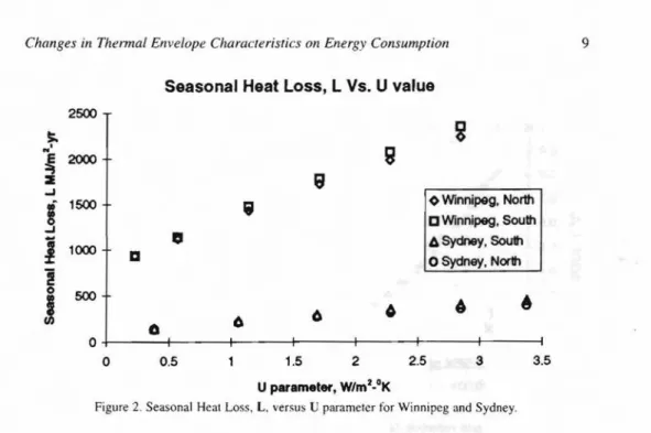
A simple heating model was developed to predict the change in annual heating load for the simulated buildings given a change in one of the thermal envelope parameters. The model consists of progressively adjusting the Seasonal Heat Loss, L, using solar and internal gain reduction factors.L is a measure of the heating required in a perime-ter zone having no solar and no inperime-ternal gains. The Seasonal Heat Loss, L, for the perimeter zones can be calculated using the transmission characteristics of the build-ing envelope, specifically U. The relationship between Seasonal Heat Loss and the envelope transmission parameters, U, is linear (Equation I) and is shown in Figure 2. The slope of the lines give a general indication of climate. Winnipeg is a heating dom-inated climate whereas Sydney appears to require little heating.L can be written as:

W/m2 where:

U= U value parameter, W/m2_-oK

b_Ojand b_1jare climate dependent coefficients j = {East, West, North, South}

Solar gains in buildings tend to reduce the annual heating system loads. The Solar Gain Reduction Factor, SGRF, was defined as the ratio of the annual heating system load including solar gains (but not including internal gains),Lv,and the Seasonal Heat Loss, L. SGRF represents the amount of solar gain in the perimeter zones and is a function of the solar parameter, V, and the Seasonal Heat Loss. Figure 3 shows the relationship between SGRF and the V parameter for Winnipeg and Sydney. The curves describing SGRF are shifted for each orientation. A single curve was fitted to predict SGRF for all the locations in the Canadian database (Cornick and Sander 1994). For each location in the database four sets of coefficients, one for each

Changes in Thennal Envelope Characteristics on Energy Consumption

Seasonal Heat Loss, L Vs. U value

2500 ｾ

ｾ

Nt

9

ｾ

2000 ｾ ..J

o

Winnipeg, North

t

1500 CWinnipeg, South ..J

.,

-

6 Sydney,Sou1h

:!

1000

_a

oSydney, Nor1h

!

0 ₅₀₀

J

6

"

•

6 6

e

0 0 0.5 1.5 2 2.5 3 3.5 U parameter, W/m2_.oK

Figure 2. Seasonal Heat Loss, L, versus U parameter for Winnipeg and Sydney.

9

tation, were generated, The same fonn of the equation was used to predict SGRF for locations in the Australian database, only the coefficients changed. The equation pre-dicting SGRF is:

SGRF = L.,IL =

rev,

L) = 1/(1 +<XIj

*

x+U2j

*

x2+<X3j

*

x3) (2)

where: x=VIL

alj' a2j' a3j are location dependent coefficients j = {East, West, North, South}

Relationship ot SGRF to Solar Parameter V

0,9

Xxx

0.8 _ｾ Location: Winnipeg X 0.7

_>s<

ｾ

s

0.6 ｾ ..J _ｘｾ

u:

0.5 a: X

ｾ

0.4

-0.3

-

-ｉｘｎｾｴｨ

I

-0.2 -South

- ...

0,1

-

-O - + - - - + - - - - I - - - + - - - + - - - - + - - - i

o

0,0002 0,0004 0.0006 0.0008 0,001 0,0012 VA.

Figure 3(a). Solar gain reduction factor versus solar parameter, V, for North and South orientations of Winnipeg.

10 Changes in Thermal Envelope Characteristics on Energy Consumption

Relationship of SGRF to Solar Parameter V

0.008 0.007 0.006 0.005 Location: Sydney

..

0.003

...

0.002

.

•

•

..

0.001

ｾ

X X

...

_.

0.9 0.8 0.7

:l

0.6

u:

0.5 a: ｾ 0.4 0.3 0.2 0.1 ＰＫＭＭＭｾｾｾＢｾＪ｟ＱｍＭＭｾＱＭＭＭＭＭＭｩｾＱＭＭ］ＭＭＭＫ［ｅＭＭｾＭＭｉｴＭｩ o 0.004 VIL

Figure 3(b). Solar gain reduction factor versus solar parameter, V, for Nonh and South orientations of Sydney.

Similarly, internal gains in buildings also contribute to the reduction of annual heat-ing loads. The internal gain reduction factor, IGRF, was defined as the ratio of the annual heating load including internal gains (but not including solar gains), L_{w '}to the Seasonal Heat Loss, L. This factor represented the amount of internal gain in the perimeter zones and is a function of the internal parameter Wand the Seasonal Heat Loss. Figure 4 shows the relationship between IGRF and the W parameter for Winnipeg and Sydney. Internal gains are the same for the cardinal orientations there-fore the curve describingIGRFis independent of orientation. A single curve was fit-ted to predictIGRFfor the Canadian database locations (Cornick and Sander 1994). Again the same form of the equation was used to predict IGRFfor locations in the Australian database. New coefficients were generated for the Australian locations. The equation predictingIGRFis:

IGRF = LwfL = feW, L) =･ｸｰＨｾｬ

*

Y+ｾＲ

*

y2+ｾＳ

*

y3) (3)

where:

y=WIL

ｾ I' ｾＲＧ ｾＳ are location dependent coefficients

The annual heating system load, Q, for a perimeter zone can be calculated as the product of the seasonal heat loss, L, and the solar gain and internal gain reduction fac-tors,SGRFandIGRF(Equation 4).

Changes in Thernwl Envelope Characteristics on Energy Consumption 11

Q

=L

*

SGRF

*

IGRF8 W/m2

₍₄₎

Relationship of IGRF to Internal Load Parameter, W

0.9

,

0.8 Location: Winnipeg ｾ 0.7 _ｾ

j

0.6

*'

)Go

u:

0.5

>w-a: S2 0.4 X"X.

ｉｘｎｯｲｾ

_I

0.3

_Xk.

_{ﾷｓｯｵｾ} 0.2 )f X-0.1 _)f 0 0 0.02 0.04 0.06 0.08 0.1 0.12 WIL

Figure 4(a). Internal gain reduction factor versus internal gain parameter, W, for North and South orienta-tions of Winnipeg.

Relationship of IGRF to Internal Load Parameter, W

0.9 0.8 Location: Sydney 0.7

1

0.6

u:

0.5 a:

_ｾ

S2 0.4

x..

0.3 X

.

0.2

Mx)f

0.1

ｾ

_ｾＧｊＨ X ｯＫＭＭＭＫＭＭＭＫＭＭＭＫ｟ＭＭＫ｟ＭＭＭＭＧｾｾＭＭＭＫ｟ＭＭ｟ｬ｟Ｍ｟Ｊｬ o 0.1 0.2 0.3 0.4 0.5 0.6 0.7 0.8 WIL

Figure 4(b). Internal gain reduction factor versus internal gain parameter, W, for North and South orienta-tions of Sydney.

8The model used in the Canadian energy code contained a Gain Interaction Factor, GIF, to account for the interaction of internal and solar gains (Cornick and Sander, 1994). The model described here however was adequate for predicting heating system loads for the colder Australian climates since the heating system loads for Australia were relatively small. The Gain Interaction Factor was not used as part of the Australian model. Consequently GIF was not used for the comparative study described in this paper.

12 Changes in Thermal Envelope Characteristics on Energy Consumption

Figure 5 compares heating loads calculated using the model and those obtained from the DOE2.IE simulations. The model predicts the annual heating system loads to within 10% for typical heating loads.

Calculated Annual Heating Vs. DOE-2, MJ/m2

2500 Location: Winnipeg 2000 I&. a::

52

1500 I&. a::

ｾ

•

1()()() _{X North} ..J II _South

a

500 ••••• ·10% 1:1 0 0 500 1()()() DOE-2 1500 2000 2500

Figure Sea). Comparison of predicted heating loads versus DOE2.1 E simulations for Winnipeg.

Calculated Annual Heating Vs. DOE-2, MJ/m2

Location: Sydney X North South ••••• ·10% 1---1:1 450 400 I&. 350

ｾ

300 I&. ₂₅₀ a::

ｾ

200 ..J ₁₅₀ II

a

100 50 0 0 50 100 150 200 250 300 350 400 450 DOE-2

Figure S(b). Comparison of predicted heating loads versus DOE2.\ E simulations for Sydney.

Of critical importance was how well the model predicted changes in annual heat-ing loads due to changes in the envelope parameters. One reason for this was that in the Canadian code the prescriptive levels were selected by minimizing the sum of incremental construction costs and the present value energy cost for different

con-Changes in Thermal Envelope Characteristics on Energy Consumption 13

struction options (Sanderet ai., 1995). Another reason was that the model forms the

basis for the trade-off calculations for the Canadian code and is being reviewed for use in the Australian code. The trade-off path allows the designer to adjust the V and U parameters to satisfy an energy budget therefore the model must accurately predict the effect of a change in U and V. Figures 6, 7, and 8 show how the model predicts changes in heating due to changes in envelope parameters, U, V, and W. The figures compare derivatives dQ/dX (X = {U, V, W}) calculated from the simulations with those derived from the model. The slopes calculated from the model compare well with those calculated from the DOE2.1 E simulations.

dQ/dU calculated Vs. dQ/dU from DOE-2

Location: Winnipeg X Winnipeg, North Winnipeg, South ••••• ·10% 1---1:1 700 600

I

500400

1

300 ::::l

ｾ

200

"

100 0 0 100 200 300 400 dQldU DOE-2 500 600 700

Figure 6(a). Comparison of change in healing for change in U,dQ/dUfor Winnipeg.

dQ/dU calculated Vs. dQ/dU from DOE-2

Location: Sydney X Sydney, North Sydney, South ••••• ·10% 1---1:1 160 140 120

j

100

ｾ

.!! ₈₀ ｾ ::::l ₆₀

ｾ

"

40 20 0 0 20 40 60 80 100 dQldU DOE-2 120 140 160

14 Changes in Thennal Envelope Characteristics on Energy Consumption

dQ/dV calculated Vs. dQ/dV from DOE-2

Location: Winnipeg X Winnipeg, North Winnipeg, South ••••• ·10% 1---1:1 -2000 -1000 -3000 -2500 ·1500 -1000 -1500 -2000 -2500 -3000 dQ/dVDOE-2

Figure 7(a). Comparison of change in heating for change in V, dQ/dV for Winnipeg.

dQ/dV calculated Vs. dQ/dV from DOE-2

-500 -400 Location: Sydney -300 -200 x Sydney,North Sydney, South ••••• ·10% - - - 1 : 1 ·100 -150 -200 -250 -300 -350 -400 -450 -500 dQ/dVDOE-2

Figure 7(b). Comparison of change in heating for change in V, dQ/dV for Sydney.

COOLING

A two part model was developed to predict the change in cooling system loads due to a change in U, V, or W. The first part of the model calculates the Base Cooling Load,

Co' The Base Cooling Load was defined as the cooling system load for a perimeter zone having no transmission losses or gains (i.e. U= 0). In the absence of transmis-sion gains or losses any loads introduced to the interior must be removed when cool-ing is required. Consequently the base coolcool-ing load is linearly proportional to the V and W parameters (Equation 5). This is shown in Figure 9.

Changes in Thermal Envelope Characteristics all. Enel:r;y Consumption 15

Co=aoj+alj

*

V+a2j

*

W W/m2 (5) dQ/dW calculated Vs. dO/dW from DOE-2

Location: Winnipeg X Winnipeg, North Winnipeg, South ••••• -10% - - - 1 : 1 -2 -4 -8 -6 -10 -12 -14 -4 -6 -8 -10 ·12 -14 dQldWDOE-2

Figure X(a). Comparison of change in heating for change in W. dQ/dW for Winnipeg.

dQ/dW calculated Vs. dO/dW from DOE-2

-6 -5 Location: Sydney -4 ·3 -2 X Sydney, North Sydney,South ••••• '10% - - - 1 : 1 -1 -2 -3 -4 ·5 -6 dQldWOOE·2

Figure 8(b). Comparison of change in heating for change in W, dQ/dW for Sydney.

This simple linear model was an adequate predictor of the cooling system loads when the system loads became large. This was because, unlike heating, cooling sys-tem loads are primarily the result of solar and internal gains and the effect of U on cooling is small. In Canada, however, the cooling system loads were found to be small. Some of the cooling loads were small enough that the loads were primarily the result of the minimum ventilation requirements and the choice of HVAC system. The

calcu-16 Changes in Thermal Envelope Characteristics on Energy Consumption

Cooling Load at various values of V and W for U

=

0.23 w/m2

_

oK

1400

Location: Winnipeg South 1200 N

ｾ

1000 2

1

_oJ 800

r

8

600 0 ＭＫＭｷｾｯｷｉｭＲ ili ""-w= 13wlm2 ='_c 400 c _{-IJr-w'"' 27 wlm2}

<

ｾｷ］ＵＳｷｉｭＲ 200 _{_w=80wIm2} -9-w= 107wlm2 0 0 0.2 0.4 0.6 0.8 Solar Parameter, V

Figure 9(a). Cooling load at U=0.23 for varying values of V and W for Winnipeg. South. Cooling Load at various values of V and W for

U

=

0.39 w/m2

_.oK

2500

Location: Sydney North

2000

ｾ

_:::E

1

1500 oJ c c

1

₀ 1000 "i -+-w=OwIm2 =' _{""-w=41 wlm2} c c

<

-IJr-w:o 71 wlm2 500 _ w : o 100w1m2 0 0 0.2 0.4 0.6 0.8 Solar Parameter, V

Changes in Thermal Envelope Characteristics on Energy Consumption 17

lation ofCo was slightly modified to reflect this minimum condition9 .A similar min-imum cooling load was predicted for Australia and was observed to occur in the cool-er locations such as Canbcool-erra. The revised equation for the base cooling load is shown below (Equation 6).

(6)

where:

CmiRis the minimum cooling load for a particular climate location.

aOj' alj anda2j are climate and orientation dependent coefficients.

j ={East, West, North, South}

The second part of the cooling model accounts for transmission gains or losses across the envelope. An Envelope Correction Term, !lC, was defined. The correction term either decreases or increases the cooling system load and is climate dependent. Figures lO(a) and (b) show the change in cooling due to a change in U for mild and cold climates. An increase in the value of U produced a decrease in the cooling sys-tem load. The U value effect increases with increased cooling loads until it becomes almost linear. In cold climates, such as those in Canada, the effect of transmission loss-es on heating differs by an order of magnitude from the effect of transmissions loss on cooling. The advantage of free cooling are more than offset by increased heating sys-tem loads.

Effect of U parameter on Cooling

20 H Location: Winnipeg ::::l ₀ E ｾ _{<><> <>- <><>}

_<><fIIJ

_{<><> ＼＾＼＾＼＾ｾ＼＾ <><>0}1_ｾ 1200 1400

g

::J -20 D <><> <> _<>

.

ｾ

_ict:l

_{cc CQII CD}

_crw

::::l. Ｑｩｾ -40 ｾ DC Cca . . A . 666 DC Cta CD

ｲｾ

AU

=

U - 0.23 W/m'-"K 66 66& 66 Cc C _C

8 -

-00 :«" Xxx Ｖｾ Ｈｊｾ _<>0.34068 :« :« xx ｘｘｾ 66 Ｖｾ 6

.so

:«:It:«:« XX ｘｾ 6 66 6

i

-80 CO.90848 :«:«. :«:« xx XX)( 6 Ｚﾫｾ Xx Xx 61.47628 _{:«:« :«:«z x}

!

-100 X 2.04408 :«:« X C _:«2.61188 :«:« :« :« ·120

Cooling Load at U.0.23,MJ/m2·yr

Figure )O(a). Effect of envelope transmission on cooling loads for Winnipeg, South.

9Note that the HVAC system selected and the minimum ventilation requirement would also result in a min-imum heating load, however in Canadian climates this minmin-imum was never reached.

18 Cfumges in Thermal Envelope Characteristics on Energy Consumption

Effect of U parameter on Cooling

1..- 6U - U - 0.39W/m'-oK

ｾ

500 0 1000 1500 200100.673 251 0 _{0 0} 0 01.305 0 _61.9 00 0 0 rI 08 X2.463 0 0 0 0

8

ｯｾ

i

0 _ｯｾ 0 IJIJ 0 ( :1:2.994 6 6 0 6 _IJ Ｖｾ IJ 6

ｾ

6 6

ｾ

6 6 6X₆ 6 6Ji _IJ [JJ

ｾ

ｾ

X:I: _X:I: .:1: X

>sf

X _ｾ

•

:I: 6 X X Xx

X :I: :I: X :I: :I: :I: :I: :I:

L

:I: :I: :I: :I: 6 :I: :I: 6 20 0 II ::I _-20 E ｾ -40 ::r II ｾ

_..eo

::I,

ｾｾ

-80 S::E

8

a; -100 o ｾ SO _-120

8

ｾ -140

!

_-160 C Location: Sydney -180

Cooling Load at U • 0.39, MJlm2-yr

Figure 1O(b). Effect of envelope transmission on cooling loads for Sydney, North. Effect of U parameter on Cooling

350 Location: :I: DalWln 6U = U - 0.39 W/m'-"K

j

is 300 250 200 150 100 50 X

o

500 1000 :I: X :I: \:1::1: X ｾｘ 6 6 6 6 IJ OIJ IJ

o to

_o

1500 2000 2500 3000 3500 00.673 IJ1.305 61.9 X 2.463 :1:2.994 4000 4500 50( ·50

Cooling Load atU.0.39, MJlm2_.yr

Figure lO(c). Effect of envelope transmission on cooling loads for Darwin. North.

Figure lO(c) shows the envelope effect in a hot climate, such as Darwin. In Darwin the ambient temperatures are mostly above the cooling setpoint. Decreasing the value of U decreases the amount of heat transferred into the building thus lowering the cool-ing system load. Like cold climates however the effect of envelope gains is small. Unlike cold climates the effect of reducing the amount of insulation in the envelope decreases as cooling loads become larger. Reducing cooling system loads by increas-ing the amount of insulation in the envelope has a marginal payback in hot climates. In fact in mild climates, where ambient temperatures are never very far from comfort,

Changes in Thermal Envelope Characteristics on Energy Consumption 19

decreasing the value of U can actually have a marginal adverse effect on energy con-sumption (Thomas and Prasad, 1995). In these climates with small heating needs, the energy reduction for heating due to increased insulation can be less than the increase in cooling energy due to loss of free cooling.

A general form for the envelope correction term was defined as:

W/m2

₍₇₎

where:

a 3janda4jare climate and orientation dependent coefficients. Co is the base cooling load for orientation

j

=

{East, West, North, South}

This general form worked well for both hot and cold climates. A simplification of the envelope correction term can be made for locations having net loss through the envelope i.e. having a graph similar to that in Figures lO(a) and (b). In this case the cooling curves are cut off atCmin'the minimum cooling system load for that location. The Cmin cut off was a boundary condition used to eliminate one of the coefficients from the general form (Equation 7). The simplified Envelope Correction Term is shown below (Equation 8).

(8)

Since all Canadian locations exhibited the same ｾｃＯｾｕ profile as that in Figure 10(a) the simplified correction term (Equation 8) was used to calculate the envelope correction term for Canadian National Energy Code for Buildings. Australian loca-tions span the range from hot climates, where net transmission gains occur across the envelope, to cooler climates, such as Canberra where net losses occur across the enve-lope. Sinceｾｃ could not be simplified for hot climates such as Darwin the Australian Energy Code trade-off calculations used the more general form for the envelope cor-rection term (Equation 7).

Cooling system loads for a perimeter zone are calculated as the sum of the Base Cooling Load,Co'and the Envelope Correction Term,ｾ｣Ｎ Where a minimum cooling load exists the cooling system load is greater of_{C min} and the sum of Co and ｾｃ

(Equation 9).

C =max(Cmin, Co +ｾｃＩ W/m2

₍₉₎

'OWhen the coefficients for the general equation were solved for numerically the coefficients for locations having a minimum cooling load were such that34=-33*_{Cmin. This can also be shown algebraically by} assuming that ifC=Cmin at V=O. W=0, and U=D,thenCo=Cmin by definition. Consequently tiC must be O. Solving for this boundary condition coefficient the34 coefficient becomes -33*Cmin' In loca-tions such as DarwinCmin occurs when U=V=W=O. The correction tenn cannot be simplified for these locations.

20 Changes in Thermal Envelope Characteristics on Energy Consumption

Figure 11 compares cooling loads calculated using the model and those obtained from the DOE2.IE simulations. Of critical importance was how well the model pre-dicted changes in annual cooling loads due to changes in the envelope parameters. Figures 12, 13, and 14 show how the model predicts changes in heating due to changes in envelope parameters, U, V, and W. The figures compare the derivatives dC/dX (X = {U, V, W}), calculated from the DOE2.1E simulations with those derived from the model.

Calculated Annual Cooling Vs. DOE-2, MJ/m2

200 1400 1200 Location: Winnipeg 1000 (J <l ₈₀₀ + 0 X North (J II 600 South (J _{. , - . , , 5%} 400 1:1 1400 1200 1000 600 800 DOE-2 400 200 O ¥ - - + - - - j - - - ! - - - + - - - + - - - - f - - - !

o

Figure II(a). Comparison of cooling loads calculated using model and DOE2.1 E results for Winnipeg.

Calculated Annual Cooling Vs. DOE-2, MJ/m2

Location: Sydney ·-'--'5% X North South 2500 2000 - - - 1 : 1 1500 1000 500 2500 2000 (J 1500 <l + 0 0 II 1000 (J 500 0 0 DOE-2

Changes in Thennal Envelope Characteristics on Energy Consllmption 21

Figure 12(a) shows the predicted slopes dCldU plotted against the slopes calculat-ed from DOE2.1 E for Winnipeg. For moderate values of Co the model prcalculat-edicts the slope well, however, as Co increases the effect of U becomes progressively linear and tends to diverge from the trend predicted by DOE2.lE. Summertime transmission gains (or losses) however tend to be insignificant when compared to solar and internal gains. For the purposes of the Canadian Energy Code this error was tolerable since for Canadian climates solar and internal gains are the predominant factors in determining cooling system loads. Figure 12(b) shows dC/dU for Sydney. The cooling model pre-dicts that envelope losses have a linear effect on cooling system loads. In this case the model doesn't predict the trend for U very well. For Sydney however the effect of envelope losses on cooling system loads is negligible compared to the effect of solar aperture and internal loads. To get a quantitative feel for how much the parameters U, V, and W change the cooling system loads for a building an equivalency was calcu-lated. This equivalency calculated how much change in U or V was required to effect a change equal to a I W/m2_{change in the internal load parameter, W. Typical values}

for U, V, and W were assumed to be 2.3 W/m2_{-Ko, 0.4, and 30 W/m}2_{respectivelyl!.}

For the Australian model, a change of I W/m2_{in W (a 3% change in W) is equivalent}

to a I % percent change in North facing window area or tint (2% for the South side). In Sydney adding a layer of insulation of R_si7 would produce an increase in the cool-ing system load equivalent to 1 W/m2.Even in a hot climate, such as Darwin, the effect of envelope on cooling is small. In Darwin a layer of Rsi5 would have to be added to

the envelope to get an equivalent decrease in the cooling system loads. For the pur-pose of the Australian Energy Code the insensitivity shown in Figure 12(b) was toler-able given the overwhelming dominance of solar aperture (Thomas and Prasad, 1995). Controlling solar gains and internal load is more cost effective approach to reducing cooling system loads.

dC/dU calculated Vs. dC/dU from DOE-2

20 Winnipeg, North Winnipeg South ••••• -10 % -80 Location: Winnipeg -100 dCldU DOE·2

Figure 12(a). Comparison of change in cooling for change in U, dC/dU for Winnipeg. IIThese values assume a window to wall ratio of50%,a shading coefficient of0.8, U_{g1ass =}4.04(double glazed), and U",oll = 0.56.

22 Changes in Thermal Envelope Characteristics on Energy Consumption

dC/dU calculated Vs. dC/dU from DOE-2

20 10 -20 -25 -30 -35 -20 -30 -40 ·50 X Sydney, North Sydney.Soulh ••••• ·10% 1---1:1 -60 Location: Sydney

..,...

ｾｾＮｲＺ［ＧＦｾ

ｸｾｯ

X >0<X -45 dCldU DOE-2

Figure l2(b). Comparison of change in cooling for change in U,dC/dUfor Sydney.

-70

The slope predicting the change cooling system loads for a change in solar aperture is well predicted by the model for Winnipeg (Figure 13a). For Sydney (Figure 13b) however the slope dC/dV appears to be insensitive to solar aperture. For large cooling system loads the cooling model becomes linear with U, V, and W. The error in the solar term is due to the error introduced in correcting for envelope transmission, how-ever the slopes are predicted to within 10% of the slopes obtained from DOE2.1 E. All 144 combinations of U, V, and Ware shown in Figure 13(b) and these combinations cover the complete range of constructable buildings. The same phenomenon is appar-ent in the predictions of the change in cooling due to change in internal loaddC/dW for Sydney. Again for large cooling loads the model becomes linear with U, V, and W and an error is introduced in correcting for the envelope transmission. The cooling model still predicts dC/dW within 10% over the complete range of building con-structions.

CLIMATE CORRELATIONS

The new Canadian Energy Code was designed to be regionally sensitive. In order to permit the calculation of prescriptive requirements for locations not in the original database the heating and cooling models were extending to include climate correla-tions12. All the climate correlation equations were based on available weather data,

12The Canadian Energy Code is divided into several administrative regions each with different envelope requirements. The regions represent distinct climatic and economic regions and account for sensitivity in fuel prices and construction costs as well as climate. The provinces and territories were responsible for selecting the appropriate zones and the weather they wished to use. In fact several weather stations were selected by the provincial ministries for the Energy Code that were not among the list of locations simulat-ed. The climate correlations were used to generate the coefficients for the heating and cooling equations which subsequently appeared in the Life Cycle Costing Analysis procedure and Tradeoff specification (Sander and Cornick, 1994).

Changes in Thermal Envelope Characteristics on Energy Consumption

dC/dV calculated Vs. dC/dV from DOE-2

23 X Winnipeg, North Winnipeg, South ••••• ·10% 1:1 1000 900 800

I

700 :; 600 () ｾ 500 > 400 ｾ 0 300 'a 200 100 0 0 Location: Winnipeg 200 400 600 800 1000 dCldV DOE-2

Figure 13(a). Comparison of change in cooling for change in V, dC/dV for Winnipeg.

dC/dV calculated Vs. dC/dV from DOE-2

1800 1600 1400 Location: Sydney

j

1200 III :; ₁₀₀₀ ()

!

₈₀₀ >

ｾ

600 X Sydney,North 'a _Sydney,South 400 ••••• ·10% 200 1:1 0 0 200 400 600 800 1000 1200 1400 1600 1800 dCldV DOE-2

Figure l3(b). Comparison of change in cooling for change in V, dC/dV for Sydney.

specifically, cooling degree days, heating degree days, vertical solar radiation (VS/3), and latitude. Correlating the cooling coefficients to climate was straightforward since the cooling coefficients C_{min ,}ao, ai' a2 and a3 had some physical significance. Figure 15 shows the comparison between cooling system loads calculated using the cooling equations with coefficients generated using the climate correlations and the results from DOE2.1 E simulations for Vancouver. The difference between the predicted and simulated cooling system loads is 10%.

24 Changes in Thermal Envelope Characteristics on Energy Consumption

dC/dW calculated Vs. dC/dW from DOE-2

4 3.5 3

J

.!! 2.5 :;, j !

5

2 ｾ ｾ 1.5 0 "0 0.5 Location: .Winnipeg

x

x

Winnipeg, South ••••• ·10% 1---1:1 X Winnipeg, North 4 3.5 3 2.5 0.5 o

-<>.5

1.5 2 dCldWDOE-2

Figure 14(a). Comparison of change in cooling for change in W,dC/dWfor Winnipeg.

dC/dW calculated Vs. dC/dW from DOE-2

X Sydney, North Sydney, South ••••• ·10% 1---1:1 8 7 6 _{Location: Sydney}

I

5 '3_u

3

4 ｾ ｾ 3 0 "0 2 0 0 2 3 4 dCldWDOE·2 5 6 7 8

Figure 14(b). Comparison of change in cooling for change in W,dC/dWfor Sydney.

Compared to the cooling equations, correlating the heating equation coefficients to climate was more complex. The seasonal heat loss, L. was simple to correlate since the coefficients bOjand b1jhave some physical significance. The coefficient bOj

repre-sents the characteristics of the selected HVAC system as well as the infiltration and ventilation losses for a specific location while b1jis a measure of the temperature of a

given location. Both these coefficients varied linearly with heating degree days. The curves predicting SGRF and IGRF were best fit curves and could not be directly cor-related to climate. Since the curves for the reduction factors were similar for each city a climate dependent parameter was derived that would shift curves for a particular

Changes in Themwl Envelope Characteristics on Energy Consumption 25

location to specific reference curve. It was then possible to correlate the parameters that shifted the SGRF and IGRF curves to weather data.

Cooling Loads from Climate Correlations Vs. DOE-2 Cooling

Loads

1000

ｾ

900

NI

.§

800

-.

:::g

700

..--600 </l s:: 0 Ｎｾ

₅₀₀

c:'<S a)

400

5

_u

300

S 0

₂₀₀

<l:: ' - '

u

100

0

0

Location: VancouverEast

200

400

600

800

..

1:1 10%

woo

C (from DOE-2) MJ/m2-yr

Figure J5. Comparison of cooling load calculated using climate correlations with loads predicted by DOE2.lE for Vancouver East orientation.

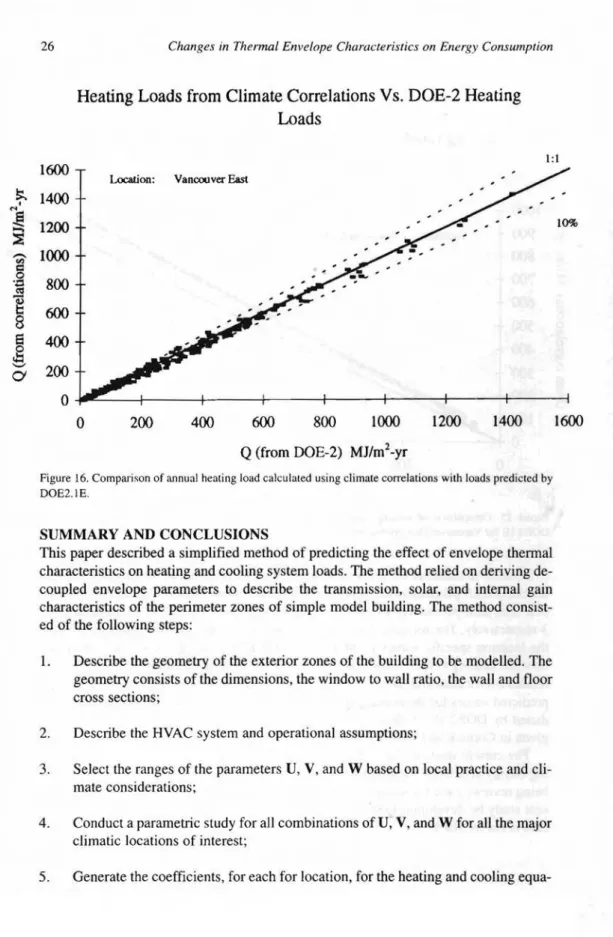
In order to calculate the reduction factors for a location not in the original database the curve shift parameters are generated from the climate data for the location in ques-tion. The shift parameters are used to modify the x and y variables of Equations 2 and 3 respectively. The reference curves for SGRF and IGRF are then used to calculate the location specific values of SGRF and IGRF. Figure 16 shows the comparison between heating system loads calculated using the heating equations with climate cor-related coefficients and the results of DOE2.1 E simulations for Vancouver. Most of the predicted values for the heating system loads are within 10% of the system loads pre-dicted by DOE2.1 E. A detailed description of the climate correlations for heating is given in Cornick and Sander (1994).

The current study is one of the steps towards developing and implementing build-ing energy efficiency standards for Australia. The results of this and other studies are being reviewed and further research is anticipated. Such research could extend the pre-sent study by developing correlations for locations for which comprehensive weather data is not available.

26 Changes in Thermal Envelope Characteristics on Energy Consumption

Heating Loads from Climate Correlations Vs. DOE-2 Heating

Loads

1:1

Location: VancouverEast 1600 !;:, ₁₄₀₀ MI .§ 1200

ｾ

... 1000

'"

c 0 800 Ｎｾ ｾ

ｾ

600

8

Ei ₄₀₀

ｾ

₂₀₀ CJ 0 0 200 400 600 800 1000 1200 1400 10% 1600

Q

(from DOE-2) MJ/m2-yr

Figure 16. Comparison of annual heating load calculated using climate correlations with loads predicted by

DOE2.1E.

SUMMARY AND CONCLUSIONS

This paper described a simplified method of predicting the effect of envelope thermal characteristics on heating and cooling system loads. The method relied on deriving de-coupled envelope parameters to describe the transmission, solar, and internal gain characteristics of the perimeter zones of simple model building. The method consist-ed of the following steps:

1. Describe the geometry of the exterior zones of the building to be modelled. The geometry consists of the dimensions, the window to wall ratio, the wall and floor cross sections;

2. Describe the HVAC system and operational assumptions;

3. Select the ranges of the parameters U, V, and W based on local practice and cli-mate considerations;

4. Conduct a parametric study for all combinations ofU, V, and W for all the major climatic locations of interest;

equa-Changes in Thermal Envelope Characteristics on Energy Consumption

tions described here;

27

6. If the database of parametric studies is large enough generate climate correla-tions to generate coefficients for locacorrela-tions not in the database;

7. Use the heating and cooling models described in this paper to predict heating and cooling system loads given values of D, V, and W.

This paper demonstrated that the methods outlined in this paper are robust. It can be used for a variety of climates, different HVACsystems, different geometry's and different operational assumptions. The method can be used to construct databases of parametric studies, climate correlations, or site specific models.

REFERENCES

AS 1668, The Use of Mechanical Ventilation and Air-conditioning in Buildings, Part 2:

Mechanical Ventilation for Acceptable Indoor Air Quality, Standards Australia, Sydney, 1991.

ASHRAE, ANSIIASHRAE Standard 62-1989. Ventilation for Acceptable Indoor Air Quality, ASHRAE, Atlanta, GA, USA, 1989.

ASHRAE. 1989 ASHRAE/IES Standard 90.I-l989, Energy Efficient Design of New Buildings

Except Low-Rise Residential Buildings. ASHRAE, Atlanta, Georgia.

Berkeley Solar Group. 1986. Regression Equations for ASHRAE Standard 90.1 Envelope

Calculations. April 30, 1986. Berkeley Solar Group, Berkeley, California.

California Energy Commission. 1990. Base Case Building Description. April 23, 1990. California Energy Commission, Sacramento, California.

Cornick, S.M., Sander, D.M. "Creating a Simplified Energy Model for Analysis of Building

Envelope Characteristics" to appear in Thermal Performance of the Exterior Envelopes of

Buildings VI Proceedings, Clearwater Beach, Florida, December 4-8, 1995.

Cornick, S.M., Sander, D.M., The Effect of Mass on the Prescriptive Levels in the Energy Code

for Buildings, Committee Paper, 31st Meeting of Standing Committee on Energy Conservation

in Buildings, Agenda 12, pp. 1181-1222, Canadian Codes Center, National Research Council of Canada, September 1995.

Cornick, S.M. Using the Calculation Method for Envelope Tradeoff Compliance for the

National Energy Code, In preparation, IRC-IR-699, National Research Council of Canada, in

press.

Cornick S.M., Sander D.M. Development of Heating and Cooling Equations to Predict Changes

in energy use Due to Changes in Building Thermal Envelope Characteristics, IRC Internal Report, IRC Internal Report, IRC-IR-656, National Research Council of Canada, I January,

1994.

Crawley,0.8.,Schliesing, J.S., Boulin, U. Standard 90.I's ENVSTD: A Tool for Evaluating

Building Envelope Designs. ASHRAE Journal, Vol. 32, No.7, July 1990, pp. 28-36.

Crawley, D.B., 1992. Development of Procedures for Determining Thermal Envelope

28 Changes in Thermal Envelope Characteristics on Energy Consumption

Report to the Institute for Research in Construction, National Research Council of Canada, Contract No. 31944-2-0002.0l-SR. November 1992, D.B. Crawley Consulting, Martin, Tennessee.

Judkoff, R.D., and Neymark, J.S., "A Procedure for Testing the Ability of Whole Building Energy Simulation Programs to Thermally Model the Building Fabric", Journal of Solar Energy

Engineering, Transactions of the ASME, Volume 117/7, February 1995.

Prasad, D.K., Thomas, Pe., Ballinger, J.A., and Morrison, Part A- Building Energy Efficiency

and Thermal Peiformance Standards for Australia, Energy Research and Development

Corporation report ERDC- 1547, March 1994.

Sander, D.M., Swinton, M.e., Cornick, S.M., Haysom, J.e. "Determination of Building

Envelope Requirements for the (Canadian) National Energy Code for Buildings" to appear in

Thermal Performance of the Exterior Envelopes of Buildings VI Proceedings, Clearwater Beach, Florida, December 4-8, 1995.

Sander, D.M., Cornick, S.M. Calculation Method for Envelope Tradeoff Compliance for the

National Energy Code, IRC Internal Report IRC-IR-657, National Research Council of Canada,

March 18, 1994.

Sander, D.M., Cornick, S., Newsham, G.R., Crawley, D.B., 1993. "Development of a Simple

Model to Relate Heating and Cooling Energy to Envelope Thennal Characteristics. " presented

at 3rd International Conference on Building Simulation. International Building Performance Simulation Association, Adelaide Australia, 16-18 August.

SRCI PIL, Development of Commercial Building Energy Code, report for Department of Energy and Minerals, Victoria 3002, Australia, July 1993.

Thomas, Pe., and Prasad, D.K., Enelgy Efficient Building Envelopes - An Australian

Perspective, to appear in Thermal Performance of the Exterior Envelopes of Buildings VI

Proceedings, Clearwater Beach, Florida, December 4-8, 1995.

Wilcox, B.A. 1991. "Development of the Envelope Load Equation for ASHRAE Standard 90.1"