HAL Id: hal-03062037
https://hal.archives-ouvertes.fr/hal-03062037
Preprint submitted on 5 Jan 2021
HAL is a multi-disciplinary open access
archive for the deposit and dissemination of
sci-entific research documents, whether they are
pub-lished or not. The documents may come from
teaching and research institutions in France or
abroad, or from public or private research centers.
L’archive ouverte pluridisciplinaire HAL, est
destinée au dépôt et à la diffusion de documents
scientifiques de niveau recherche, publiés ou non,
émanant des établissements d’enseignement et de
recherche français ou étrangers, des laboratoires
publics ou privés.
and memory-based search
Tianyi Li, Angelo Arleo, Denis Sheynikhovich
To cite this version:
Tianyi Li, Angelo Arleo, Denis Sheynikhovich. A model of a panoramic visual representation in the
dorsal visual pathway: the case of spatial reorientation and memory-based search. 2021. �hal-03062037�
A model of a panoramic visual
1representation in the dorsal visual
2pathway: the case of spatial
3reorientation and memory-based
4search
5 Tianyi Li1 , Angelo Arleo1 , Denis Sheynikhovich1* 6 *For correspondence:denis.sheynikhovich@upmc.fr(DS) 1Sorbonne Université, INSERM, CNRS, Institut de la Vision, 17 rue Moreau, F-75012 Paris,
7
France.
8
9
Abstract Primates are primarily visual animals and understanding how visual information is
10
processed on its way to memory structures is crucial to the understanding of how memory-based
11
visuospatial behavior is generated. Recent imaging data demonstrate the existence of
12
scene-sensitive areas in the dorsal visual path that are likely to combine visual information from
13
successive egocentric views, while behavioral evidence indicates the memory of surrounding visual
14
space in extraretinal coordinates. The present work focuses on the computational nature of a
15
panoramic representation that is proposed to link visual and mnemonic functions during natural
16
behavior. In a spiking artificial neuron network model of the dorsal visual path it is shown how
17
time-integration of spatial views can give rise to such a representation and how it can subsequently
18
be used to perform memory-based spatial reorientation and visual search. More generally, the
19
model predicts a common role of view-based allocentric memory storage in spatial and not-spatial
20 mnemonic behaviors. 21 22
Introduction
23Recent breathtaking advances in our understanding of rodent hippocampal memory system pave
24
the way for elucidating the organization of human spatial memory (Burgess, 2014;Moser et al.,
25
2017). One major difference between primates and rodents is the role of vision for behavior.
26
Primates are much more visual animals than rodents and understanding the link between primate
27
visual and medial temporal lobe (MTL) memory structures is an important and largely unexplored
28
open question (Meister and Buffalo, 2016). Experimental evidence indicates the existence of
29
functional and anatomical connections between these structures. Functional connections are
30
demonstrated by two principal lines of studies. First, visual behavior is informed by memory as
31
demonstrated by studies of novelty preference in both monkeys and humans (Wilson and
Goldman-32
Rakic, 1994;Manns et al., 2000;Jutras and Buffalo, 2010a). In the novelty preference paradigm,
33
the memory is assessed from looking time: well memorized stimuli are looked at less than novel
34
ones. The specific role of MTL structures in this phenomenon is derived from results showing
35
a decreased novelty preference after MTL lesions or in patients suffering from mild cognitive
36
impairment or Alzheimer’s disease, often associated with MTL dysfunction (McKee and Squire,
37
1993;Crutcher et al., 2009;Zola et al., 2013). In monkeys, restricted lesions of hippocampal and/or
parahippocampal cortices also decreased novelty preference (Zola et al., 2000;Pascalis et al., 2009;
39
Bachevalier et al., 2015). Second, the link between visual and MTL structures is manifested in
40
coherent neural activities in the two structures. For example, activity of single MTL neurons is
41
modulated by visual saccades (Sobotka et al., 1997), the onset of visual stimuli strongly affects
42
hippocampal neural responses (Jutras and Buffalo, 2010a) and hippocampal theta oscillations are
43
reset by eye movements (Jutras and Buffalo, 2010b;Hoffman et al., 2013).
44
Anatomical connections between visual and memory structures have recently been
charac-45
terized in the novel framework of the occipital–parietal–MTL pathway of visuospatial processing
46
(Kravitz et al., 2011). There are three principal stages of information processing in this pathway
47
(Figure 1A). First, the occipito-parietal circuit processes visual information through visual areas
48
V1-V6 an egocentric (retinal) frame of reference. Successive information processing in these areas
49
is thought to extract visual features of increasing complexity, including motion and depth cues and
50
relay this information to the parietal cortex. Second, a complex network of interconnected parietal
51
structures relays highly-processed visual cues to support executive, motor and spatial-navigation
52
functions. These structures include the medial, ventral and lateral intraparietal areas (MIP, VIP,
53
LIP) strongly linked with eye movements processing; the middle temporal and medial superior
54
temporal (MT, MST) thought to extract high-level visual motion cues; and the caudal part of the
55
inferior parietal lobule (cIPL), the main relay stage on the way to the medial temporal lobe. The cIPL
56
sends direct projections to the CA1 of the hippocampus as well as to the nearby parahippocampal
57
cortex (PHC). In addition, it sends indirect projections to the same structures via the posterior
58
cingulate cortex (PCC) and the retrosplenial cortex (RSC). Within this complex network, neurons
59
at different neurobiological sites have been reported to code space in a world- or object-centred
60
reference frames (Duhamel et al., 1997;Snyder et al., 1998;Chafee et al., 2007). Moreover, both
61
PCC and RSC have been repeatedly linked to coordinate transformation between egocentric and
al-62
locentric frames of reference (Vogt et al., 1992;Burgess, 2008;Epstein and Vass, 2014). Importantly,
63
information processing in this pathway is strongly affected by directional information thought to
64
be provided by a network of head-direction cells residing in several brain areas, including RSC
65
(Taube, 2007). Finally, medial temporal lobe, and in particular the hippocampus, play a key role in
66
constructing an allocentric representation of space in primates (Hori et al., 2003;Ekstrom et al.,
67
2003).
68
Given functional and anatomical connections between visual and memory structures, the
ques-69
tion arises as to the nature of neuronal representations in the dorsal visual path. In addition to the
70
well-established role of parieto-retrosplenial networks in coordinate transformations (Andersen
71
et al., 1993;Snyder et al., 1998;Salinas and Abbott, 2001;Pouget et al., 2002;Byrne et al., 2007),
72
a largely unexplored question concerns the existence of an extra-retinal neural map of the
remem-73
bered visual space (Hayhoe et al., 2003;Tatler and Land, 2011;Land, 2014). That the task-related
74
visual retinotopic space is remembered has been suggested by studies showing that when asking
75
to recall a recent visual content, eye movements (on a blank screen) closely reflected spatial
rela-76
tions of remembered images (Brandt and Stark, 1997;Johansson and Johansson, 2014). Moreover,
77
preventing subjects from making eye movements decreased recall performance (Johansson and
78
Johansson, 2014;Laeng et al., 2014). That not only the retinal egocentric space is remembered
79
but also extra-retinal map of surrounding space is stored in memory is demonstrated in studies
80
showing that during natural behavior human subjects direct saccades toward extra-retinal locations,
81
suggesting that these locations are represented in memory, potentially in an allocentric frame
82
of reference (Land et al., 1999;Hayhoe et al., 2003;Golomb et al., 2011;Melcher and Morrone,
83
2015;Robertson et al., 2016). Even though suggested by the above studies, the nature of such an
84
extra-retinal map and neural mechanisms underlying its construction and storage are currently
85
unknown.
86
The present modeling study addresses the question of how such an allocentric representation of
87
surrounding visual space can be constructed and stored by the dorsal visual path – MTL networks.
88
We propose that the existence of such a representation relies on short-term memory linking
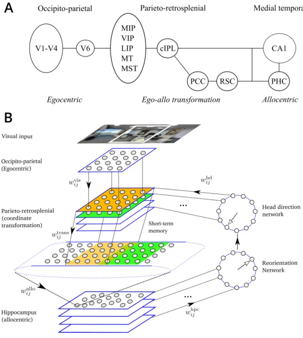
Figure 1. Model. A. Dorsal visual pathway of visuospatial information processing in primates (see text for
details). B. Schematic representation of the model. Visual features present in the limited visual field constitute the model input. The model network is composed of 6 modules: (1) Occipito-parietal (egocentric); (2)
Head-direction network; (3) Parieto-retrosplenial transformation network consists of the
coordinate-transformation network and the output layer, which encodes visual features in an allocentric directional frame and spans 2𝜋; (4) Hippocampus; (5) Reorientation network. Projections from the
occipito-parietal (visual) areas to the transformation network are topographic. Each head-direction cell activates the corresponding layer of the transformation network. Projections from the different layers of the
transformation network to the parieto-retrosplenial output layer are also organized according to head direction: any two layers project topographically to overlapping portions of the output population shifted according to head direction. Synapses between the transformation network and the parietal output network are endowed with short-term memory. Different hippocampal subpopulations project to different neurons in the
reorientation network, which in turn corrects head direction signal. Full arrows represent the flow of information in the network. Open arrows represent direction signals in the head direction and reorientation networks.
successive egocentric views and we study how the long-term memory of allocentric visual space can
90
affect behavior in spatial and non-spatial experimental paradigms. In particular, our results suggest
91
that allocentric memory effects during spatial reorientation and memory-based visual guidance
tasks can be explained by the existence of such a network.
93
Methods
94
The model is a spiking neuron network constructed to reflect information processing steps thought
95
to be performed by successive stages of neuronal processing in the primate dorsal visual path
96
described above (Figure 1A). To reflect in a simplified way the main processing stages in the pathway,
97
our model of the dorsal pathway is composed of 5 main modules or subnetworks (Figure 1B). First,
98
the module representing information processing in the occipito-parietal circuit essentially applies
99
a set of Gabor-like orientation filters to the incoming visual images, a standard assumption for
100
basic V1 processing. We do not model eye movements, and assume that a retinotopic visual
101
representations obtained at the level of V1 has been remapped, by the time it arrives into the
102
parietal cortex, to a head-fixed representation by taking into account eye position information
103
(Duhamel et al., 1997;Snyder et al., 1998;Pouget et al., 2002). Even though gaze independent,
104
this head-fixed representation is egocentric, or view-dependent, in the sense it depends on the
105
position and orientation the modeled animal (i.e., its head) in space. Second, we model the
106
directional sense by a network of cells whose activity is approximately Gaussian around their
107
preferred orientations (Taube, 2007) and that is sending projections to the parietal cortex (Brotchie
108
et al., 1995;Snyder et al., 1998). Third, both the activities of the egocentric network and the head
109
direction signal converge onto the network modeling the role of the parieto-retrosplenial network in
110
coordinate transformation. This transformation network uses head direction to convert egocentric
111
visual representations into a head-orientation-independent, or world-fixed representation. This
112
coordinate transformation is done essentially by the same mechanism as the
retinotopic-to-head-113
fixed conversion mentioned above, but in contrast to previous models it does so using low-level
114
topographic visual information. The resulting orientation-independent visual representation is
115
often referred to as spatiotopic, or allocentric, since visual features are determined a world-fixed
116
directional reference frame. Fourth, the allocentric output of the parieto-retrosplenial network
117
arrives to the hippocampus, modeled by a network of cells that learn, by a competitive mechanism,
118
allocentric visual patterns provided by the parietal network. As will be clear from the following, in the
119
context of spatial navigation these cells can be considered as place cells, whereas in a non-spatial
120
context they can be considered as representing memorised visual stimuli. Finally, the reorientation
121
module associates allocentric memories with directional reference frame and feeds back to the
122
head direction cells. The activity of this network represents the correction signal for self-orientation.
123
When the memorized information corresponds to the newly arrived one, the correction signal is
124
zero, whereas in the case of disorientation or in response to specific manipulations of visual cues, it
125
can provide fast adjustment of the self-orientation signal. In the Results section we show that a
126
similar reorientation mechanism can be responsible for behavioral decisions in spatial, as well as
127
non-spatial tasks in primates.
128
Occipito-parietal input circuit
129
The occipito-parietal network is modeled by a single rectangular sheet of 𝑁x× 𝑁yvisual neurons,
130
uniformly covering the visual field. In all simulations, except Simulation 6 below, the size of the
131
visual field was limited to 160 × 100◦, approximately representing that of a primate. The activities of
132
these visual neurons are computed in four steps. First, input images are convolved (using OpenCV
133
filter2D() function) with Gabor filters of 4 different orientations (0, 90◦,180◦,270◦) at 2 spatial
134
frequencies (0.5 cpd, 2.5 cpd), chosen so as to detect visual features in simulated experiments.
135
Second, the 8 convolution images are discretized with 𝑁x× 𝑁ygrid, and the maximal response at
136
each position is chosen, producing an array of 𝑁x𝑁yfilter responses. These operations are assumed
137
to roughly mimic retinotopic V1 processing (Heeger, 1992), transformed into a head-fixed reference
138
frame using eye-position information. Third, the vector of filter activities at time 𝑡 is normalized to
139
have maximal value of unity. Fourth, a population of 𝑁vis= 𝑁x𝑁yPoisson neurons is created with
140
mean rates given by the activity of the corresponding filters scaled by the constant maximal rate
𝐴vis(seeTable 1for the values of all parameters in the model). For a Poisson neuron with rate 𝑟, the
142
probability of emitting a spike during a small period of time 𝛿𝑡 is equal to 𝑟𝛿𝑡 (Gerstner et al., 2014).
143
Head direction
144
The head direction network is composed of 𝑁hd= 36 Poisson neurons organized in a circle, such
145
that neurons’ preferred directions 𝜙𝑘are uniformly distributed between 0 and 2𝜋. The tuning curves
146
of the modeled head-direction neurons are Gaussian with maximum rate 𝐴hdand width 𝜎hd= 8◦.
147
Thus, the rate of head-direction neuron 𝑘 when the model animal’s head is oriented in the direction
148 𝜙 is given by 149 𝑟hd𝑘 = 𝐴hdexp ( −(𝜙 − 𝜙𝑘) 2 𝜎2 hd ) (1)
Such a network generates a Gaussian activity profile centered around 𝜙. Our model does not
150
explicitly implement a line attractor dynamics hypothesized to support head direction signal (Zhang,
151
1996), but it is consistent with it. Head direction cells have been found in several brain areas
152
in rodents and primates (seeTaube, 2007, for review), and there is evidence that parietal cortex
153
receives head direction signals (Brotchie et al., 1995).
154
Parietal transformation network
155
The parietal transformation network is inspired by previous models (Becker and Burgess, 2001;
156
Byrne et al., 2007) but in contrast to them it operates directly on activities of the Gabor-like visual
157
cells. The transformation of coordinates between the head-fixed and world-fixed coordinates
158
is performed by multiple subpopulations of leaky integrate-and-fire (LIF) neurons organized as
159
two-dimensional layers of neurons (seeFigure 1). Neurons in each layer of the transformation
160
network are in a one-to-one relationship with the visual population and so at each moment 𝑡 each
161
transformation layer receives a copy of the egocentric (head-fixed) visual input. Therefore, the
162
number of neurons in each transformation layer is equal to 𝑁𝑣𝑖𝑠. Apart from the visual input, the
163
transformation network also receives input from the population of head direction cells. There
164
is a topographic relationship between the sub-populations of the transformation network and
165
different head directions: each head-direction cell sends excitatory projections to neurons only in
166
one associated layer of the transformation network. Thus, input from head-direction cells strongly
167
activates only a small subset of transformation layers which transmit visual information to the
168
downstream population. More specifically, only the layers which are associated with head directions
169
close to the actual orientation of the head are active. The number of layers in the transformation
170
network is then equal to 𝑁hd, giving the total number of neurons in the transformation network
171
𝑁trans= 𝑁vis𝑁hd.
172
Thus, in a 𝑘-th layer of the transformation network, the membrane potential 𝑣𝑖(𝑡) of the LIF
173
neuron 𝑖 in is governed by the following equation (omitting the layer index for clarity):
174 𝜏m𝑑𝑣𝑖 𝑑𝑡 = 𝑉rest− 𝑣𝑖+ 𝑔 ex 𝑖 (𝑡)(𝐸ex− 𝑣𝑖) + 𝑔 in 𝑖 (𝑡)(𝐸in− 𝑣𝑖) + 𝑅m𝐼ext (2) with the membrane time constant 𝜏𝑚, resting potential 𝑉rest, excitatory and inhibitory reversal
175
potentials 𝐸exand 𝐸in, as well as the membrane resistance 𝑅m. When the membrane potential
176
reaches threshold 𝑉th, the neuron fires an action potential. At the same time, 𝑣𝑖is reset to 𝑉reset
177
and the neuron enters the absolute refractory period Δabsduring which it cannot emit spikes. A
178
constant external current 𝐼extis added to each neuron to simulate baseline activity induced by other
179
(unspecified) neurons from the network.
180
The excitatory conductance in these neurons depends only on the visual input (and thus is
inde-181
pendent from 𝑘). It is modeled as a combination of 𝛼-amino-3-hydroxy-5-methyl-4-isoxazolepropionic
182
acid (AMPA) and N-methyl-d-aspartate (NMDA) receptor activation 𝑔ex
𝑖 = (1 − 𝛼)𝑔 ampa 𝑖 + 𝛼𝑔 nmda 𝑖 , that are 183
described by 184 𝜏ampa𝑑𝑔 ampa 𝑖 𝑑𝑡 = −𝑔 ampa 𝑖 + 𝜏ampa ∑ 𝑗∈{𝑣𝑖𝑠} 𝑤vis 𝑖𝑗 𝑠𝑗(𝑡) (3) 𝜏nmda𝑑𝑔 nmda 𝑖 𝑑𝑡 = −𝑔 nmda 𝑖 + 𝑔 ampa 𝑖 (4)
where the index 𝑗 runs over input (visual) neurons connected to it, 𝑤vis
𝑖𝑗 are the connection weights
185
and 𝑠𝑗(𝑡) = 1 if a presynaptic spike arrives at time 𝑡 and 𝑠𝑗(𝑡) = 0 otherwise. Constants 𝜏ampaand 𝜏nmda
186
determine the time scales of receptor activation.
187
In contrast, the inhibitory conductance depends only on the head-direction cells and ensures
188
that a small subset of transformation layers (i.e. those associated with nearby head directions) are
189
active. To implement it, we employ a simple scheme in which all transformation layer neurons are
190
self-inhibitory, and this inhibition is counteracted by the excitatory input from the head-direction
191
cells. Thus, the inhibitory conductance of the 𝑖-th neuron in the 𝑘-th layer is given by
192 𝜏gaba𝑑𝑔 in 𝑖 𝑑𝑡 = −𝑔 in 𝑖 + 𝐺inh+ 𝜏gaba ∑ 𝑘∈{ℎ𝑑} 𝑤hd 𝑖𝑘𝑠𝑘(𝑡) (5)
where 𝐺inh is the constant maximum amount of self-inhibition and 𝑤hd𝑖𝑘are the synaptic weights
193
of connections from the head-direction cells. In the current implementation, there is one-to-one
194
correspondence between the head-direction cells and the layers of the transformation network, so
195
𝑤𝑖𝑘= 1 only for associated head-direction cell 𝜙𝑘and 𝑤𝑖𝑘= 0 otherwise.
196
All layers of the transformation network project to the parietal output population, which codes
197
image features in an allocentric (world-fixed) directional frame. The parietal output population is
198
represented by a two-dimensional neuronal sheet spanning 360 × 100◦, that is a full panoramic view.
199
It is encoded by a grid of 𝑁allo x × 𝑁
allo
y neurons. Each layer of the transformation network projects
200
to a portion of the population according to the head direction associated with it associated with
201
this layer (seeFigure 1). Since any two nearby layers of the transformation network are associated
202
with head directions shifted relative to each other by 360◦∕𝑁
hd= 10◦, the overlap between their
203
projections on the parietal output layer is 140◦.
204
Thus, at each moment in time, a spiking representation of the current visual stream (i.e. a spiking
205
copy of the visual input, gated by the head direction cells) arrives to the allocentric neurons spatially
206
shifted according to the current head direction. For example, if two egocentric views (each spanning
207
160◦) are observed at head directions −45◦and 45◦with respect to an arbitrary north direction,
208
these two views arrive at the allocentric population spatially shifted relative to one another by 90◦,
209
so that the activated neurons in the allocentric population span 230◦. To ensure that subsequent
210
snapshots are accumulated in time (e.g. during head rotation), the synapses between neurons in
211
the transformation layers and the allocentric population are endowed with short-term memory,
212
implemented by a prolonged activation of NMDA receptors (Durstewitz et al., 2000). Such synapses
213
result in a sustained activity of allocentric output neurons during a period of time sufficient for
214
downstream plasticity mechanism to store information from accumulated snapshots.
215
The membrane potential of the 𝑖-th neuron in the allocentric output population is governed by
216
Equation 2with the synaptic conductance terms determined as follows. First, the excitatory AMPA
217
conductance is given byEquation 3but with the input provided by transformation network neurons
218
via weights 𝑤trans
𝑖𝑗 . Second, the NMDA conductance is described byEquation 4, but with the synaptic
219
time scale increased by a factor of 6. This is done to ensure sustained activation of the output
220
neurons upon changes in the visual input. Third, inhibitory input is set to zero for these neurons.
221
Learning the weights in the transformation network
222
The connection weights 𝑤vis
𝑖𝑗 from the visual neurons to the parietal transformation cells and 𝑤
trans
𝑖𝑗
223
from the parietal transformation cells to the parietal output neurons are assumed to be learned
224
during development by a supervised mechanism, similar to the one proposed to occur during
sensory-motor transformation learning (Zipser and Andersen, 1988;Salinas and Abbott, 1995). In
226
this models it is proposed that when an object is seen (i.e. its retinal position and an associated
227
gaze direction are given), grasping the object by hand (that operates w.r.t. the body-fixed reference
228
frame) provides a teaching signal to learn the coordinate transformation. A similar process is
229
assumed to occur here, but instead of learning body-based coordinates using gaze direction, the
230
model learns world-fixed coordinates using head direction.
231
More specifically, synaptic weights in the coordinate-transformation network were set by the
232
following procedure. First, the network was presented with an edge-like stimulus at a random
233
orientation and at a randomly chosen location in the visual field. Second, upon the stimulus
234
presentation, the head direction was fixed at a randomly chosen angle 𝜙. Third, neurons in the
235
transformation layers associated with the chosen head direction were activated with the average
236
firing rates equal to the rates of the corresponding visual neurons, while neurons in the parietal
237
output layer were activated with the same average rates but shifted according to the chosen head
238
direction (representing the teaching signal). Fourth, the synaptic weights in the network were set
239
according to the Hebbian prescription:
240 𝑤vis 𝑖𝑗 = 𝑟 trans 𝑖 𝑟 vis 𝑗 (6)
𝑤trans𝑖𝑗 = 𝑟trans𝑖 𝑟allo𝑗 (7)
where 𝑟vis
𝑖 , 𝑟
trans
𝑖 and 𝑟
allo
𝑖 are the mean firing rates of the corresponding visual neurons, transformation
241
network neurons and parietal output neurons, respectively. Fifth, the weight vector of each neuron
242
was normalized to have the unity norm. This procedure has been performed for edge-like stimuli
243
at 4 different orientations (corresponding to 4 Gabor filter orientations), placed in the locations
244
spanning the whole visual field and at head directions spanning 360◦. Synaptic weights (Equation 6
-245
7) were fixed to the learned values prior to all the simulation presented here. No updates were
246
performed on these weights during the simulations.
247
Hippocampal neurons
248
As a result of the upstream processing, neuronal input to the hippocampus represents visual
249
features in an allocentric directional frame. Neurons in the parietal output population are connected
250
in an all-to-all fashion to the population of modeled hippocampal cells and the connection weights
251
that are updated during learning according to an spike-timing-dependent plasticity (STDP) rule
252
below. In addition, lateral inhibition between hippocampal neurons ensures a soft winner-take-all
253
dynamics, such that sufficiently different patterns in the visual input become associated with small
254
distinct subpopulations of hippocampal neurons.
255
Thus, the membrane equation of the 𝑖-th hippocampal neurons is given byEquation 2. The
256
excitatory conductances are given byEquation 3-4, but with the input provided by the parietal
257
output neurons via weights 𝑤allo
𝑖𝑗 . Upon the initial entry to a novel environment these weights are
258
initialized to small random values. During learning, the amount of synaptic modification induced by
259
a single pair of pre- and post-synaptic spikes is given by
260 𝑑𝑤allo 𝑖𝑗 𝑑𝑡 = 𝐺max [ 𝑎pre𝑗 𝑠𝑖(𝑡) − 𝑎post𝑖 𝑠𝑗(𝑡)] (8) where 𝑠𝑖(𝑡) and 𝑠𝑗(𝑡) detect pre- and post-synaptic spikes, respectively, and
261 𝑑𝑎pre𝑗 𝑑𝑡 = − 𝑎pre𝑗 𝜏pre + 𝐴+𝑠𝑗(𝑡) 𝑑𝑎post𝑖 𝑑𝑡 = − 𝑎post𝑖 𝜏post + 𝐴−𝑠𝑖(𝑡) (9)
The inhibitory conductance of the hippocampal neuron is governed by the following equation:
262 𝜏gaba𝑑𝑔 in 𝑖 𝑑𝑡 = −𝑔 in 𝑖 + 𝜏gaba ∑ 𝑗∈{hpc} 𝑤inh 𝑖𝑗 𝑠𝑗(𝑡) (10)
in which 𝜏gabadetermines the time scale of synaptic inhibition as before, and the weights 𝑤inh
𝑖𝑗 = 𝑊inh
263
are constant and ensure that each hippocampal neuron inhibits all other hippocampal neurons
264
proportionally to its activity.
265
The hippocampal circuit is complex and consists of several interconnected populations. In our
266
simple model of hippocampal activity we consider only the first stage of hippocampal processing of
267
visual information that is likely to be the CA1, which receives direct projections from the entorhinal
268
cortex, an input gateway to the hippocampus.
269
Reorientation network
270
During one continuous experimental trial (e.g. an exploration trial in novel environment or an
271
observation of a novel image on the screen), the reference frame for head direction is fixed and all
272
processing operations in the network are performed with respect to the origin of this reference
273
frame. In particular, an allocentric information stored by the hippocampus as a result of the trial
274
can be correctly used for future action only if the origin of the reference frame is stored with it.
275
Therefore, if in a subsequent trial, the actions to be performed require memory of the previous one,
276
the network should be able to recover the original directional reference (this of course can happen
277
only the visual information received at the start of the trial is considered familiar). Reorientation is
278
the process by which the origin of the stored reference frame is recovered.
279
Our model of this process rests on the assumption that it is automatic, fast, bottom-up, and
280
does not require costly object/landmark processing. The support for this assumption comes from
281
a large body of reorientation studies in many animal species including primates, showing that
282
object identities are ignored during reorientation (Cheng and Newcombe, 2005). The conditions in
283
which most of the reorientation studies were performed usually are such that there is no single
284
conspicuous point-like cue in the environment that can be reliable associated with a reference
285
direction. For example, in many studies the directional cues come from the geometric layout of the
286
experimental room. Lesion studies in rats suggest that reorientation in such conditions requires
287
an intact hippocampus (McGregor et al., 2004). Furthermore, we propose that this reorientation
288
network is active all the time, in contrast to being consciously “turned on” when the animal “feels
289
disoriented”. Therefore, we expect that its effects can be observed even when no specific
disorien-290
tation procedure was performed. In particular, we suggest in the Results that a manipulation of
291
objects on the screen can result in automatic corrections of directional sense that can be observed
292
during visual search.
293
The reorientation network in the model is organized similarly to the head-direction network and
294
consists of 𝑁reneurons with preferred positions uniformly distributed on a circle. Therefore, the
295
difference between two nearby reorientation cells is Δ𝜙 = 2𝜋∕𝑁re. The membrane potential of the
296
𝑖-th reorientation neuron is described by the LIF equation (Equation 2). Excitatory conductances
297
are described byEquation 3-4with the input to the neuron provided by hippocampal place cells via
298
weights 𝑤hpc𝑖𝑗 . There is no inhibition in the network, and so the inhibitory conductance is set to 0.
299
The ability of the network to perform reorientation is determined by afferent connection weights
300
from the hippocampal cells, which are determined as follows.
301
Since all allocentric information learned during a trial is linked to the same directional frame, all
302
hippocampal cells learned during the trial are connected to a single neuron of the reorientation
303
network, the one with the preferred direction 0◦(Figure 2). The connection weights between the
304
hippocampal cells and the neuron are updated using STDP rule,Equation 8-9(this is not essential
305
for the model to work, so that setting the weights to a constant value will give similar results). Once
306
the training trial is finished, 𝑁𝑟𝑒copies of the learned hippocampal population are created, each
307
corresponding to a separate neuron in the reorientation network. In each copy, all cells have the
308
same input and output weights as the corresponding cells in the original population, but their
309
connection profile is different. In particular, the copy that corresponds to the reorientation neuron
310
with preferred direction Δ𝜙 is connected to pre-synaptic cells are shifted by the same angle in the
311
topographically-organized allocentric layer (Figure 2). In machine learning literature, this technique
is called “weight sharing” and it allows to achieve translation invariance for detection of objects in
313
images. Here, we apply a similar technique in order to detect familiar snapshots and head direction
314
associated with them.
315
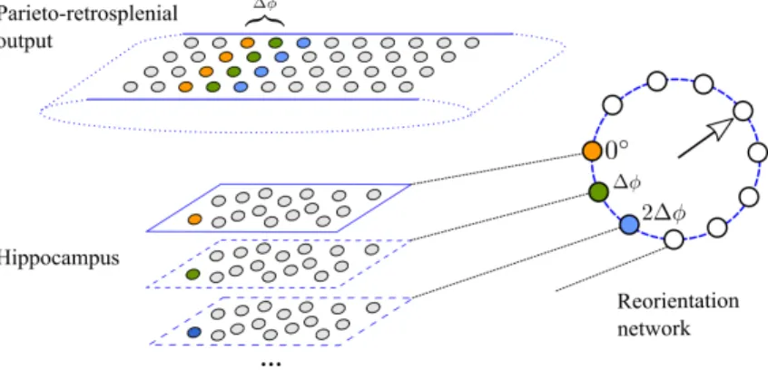
Figure 2. Implementation of the reorientation network. Top: the output population of the parieto-retrosplenial
network. Bottom: hippocampal cells. The population outlined by full lines is the original population learned during training. As a result of learning, the hippocampal cell shown in orange is connected to the presynaptic cells of the same color (connection weights not shown). All cells in the original population are connected to a single cell (𝑜◦) in the reorientation network (Right). The hippocampal populations outlined by dashed lines are
copies of the original population that implement weight sharing: the hippocampal cell shown in green (blue) has the same connection weights as the orange cell, but it is connected to pre- and post-synaptic cells shifted by Δ𝜙 (2Δ𝜙). The number of copies of the original hippocampal population is the same as the number of neurons in the reorientation network.
Suppose, for example, that as a result of learning during a trial, a hippocampal cell is associated
316
with 4 presynaptic cells in the output layer of the transformation network (cells shown in orange in
317
Figure 2). Suppose further that during an inter-trial interval the head direction network has drifted
318
(or was externally manipulated), so that at the start of the new trial the internal sense of direction
319
is off by 2Δ𝜙. When the animal sees the same visual pattern again, it will be projected onto the
320
allocentric layer shifted by the same amount (blue cells inFigure 2). This will in turn cause the
321
hippocampal subpopulation that includes the blue cell to be most strongly active, such that the
322
activity peak of the reorientation network signals the orientation error. The reorientation is then
323
performed by readjusting the head direction network to minimize the reorientation error. In the
324
current implementation this is done algorithmically by subtracting the error signal from the actual
325
head direction, but it can also be implemented by attractor dynamics in the head direction layer.
326
Simulation details
327
The spiking artificial neural network model described above was implemented using Python 2.7
328
and Brian 2 spiking neural network simulator (Stimberg et al., 2019). The time step for neuronal
329
simulation was set to 1 ms, while the sampling rate of visual information was 10 Hz, according
330
to the proposals relating oscillatory brain rhythms in the range 6–10 Hz to information sampling
331
(Hasselmo et al., 2002;Busch and VanRullen, 2010). At the start of each simulation, the weights
332
𝑤allo
𝑖𝑗 and 𝑤
hpc
𝑖𝑗 were initialized to small random values (the other weights were trained as described
333
earlier and fixed for all simulations), seeFigure 1B. Parameters of the model are listed inTable 1,
334
and the sections below provide additional details of all simulations.
335
Simulation 1: Egocentric-allocentric transformation
336
The first simulation was inspired by the study ofSnyder et al.(1998), in which monkeys observed
337
visual stimuli at identical retinal locations, but for different orientations of the head with respect
338
to the world, in order to assess whether parietal neurons were modulated by the allocentric head
339
direction. Thus, in this simulation, the head direction angle 𝜙 was varied from −50◦to 50◦in 100
340
sessions. For each trial of a session, the mean rates of the head-direction neurons were calculated
Parameter Value Description
Neuron numbers 𝑁x× 𝑁y 80 × 50 Parieto-occipital network size
𝑁hd 36 Head direction network size
𝑁allo x × 𝑁
allo
y 180 × 50 Parietal output layer size
𝑁re 36 Reorientation network size
Mean amplitudes in the input populations
𝐴vis 100 Spikes/s., Maximum rate of the parieto-occiptal network
𝐴hd 100 Spikes/s., Maximum rate of the head-direction network
Parameters of the LIF model
𝑉rest -65 mV, Resting potential
𝑉th -55 mV, Spiking threshold
𝑉reset -65 mV, Reset potential
𝐸ex 0 mV, Excitatory reversal potential
𝐸in -80 mV, Inhibitory reversal potential
𝐸in 250 mΩ, Membrane resistance
Δabs 1𝑎−𝑐, 2𝑑 ms, Absolute refractory period
𝛼 0.9𝑎,𝑏, 0.3𝑐,𝑑 Balance between AMPA and NMDA receptor
𝜏ampa 5 ms, AMPA receptor time scale
𝜏nmda 100𝑎,𝑐,𝑑600𝑏 ms, NMDA receptor time scale
𝜏x 2.5 ms, NMDA receptor time scale
𝜏m 10𝑎,𝑐,𝑑, 20𝑏 ms, Membrane time scale
𝜏gaba 10 ms, GABA receptor time scale
𝐼ext 20𝑎−𝑐, 40𝑑 mA, External input current
𝐺inh 2 Self-inhibitory conductance
STDP 𝐺max 0.05𝑐, 0.1𝑑 Maximal weight change
𝐴+ 0.005 Maximal potentiation amplitude
𝐴− 𝐴+x 1.05 Maximal depression amplitude
𝜏pre 20 ms, Potentiation time scale
𝜏post 15𝑐, 17.5𝑑 ms, Depression time scale
Other parameters
𝜎hd 8◦ Tuning curve width of head direction cells
𝑊inh 1.0 Lateral inhibition weight in the hippocampal population
Table 1. Parameters of the model. a, Occipito-parietal circuit. b, Parieto-retrosplenial transformation network.
c, Hippocampus. d, Reorientation network.
according toEquation 1and fixed for the rest of the trial. The stimulus (vertical black bar, width:
342
10◦) was shifted horizontally across the midline of the visual field (160 × 100◦) from left to right in 1◦
343
steps, such that it remained at each position for 100ms. The neuronal spikes were recorded from
344
the occipito-parietal network, the parieto-retrosplenial transformation network and its output layer,
345
for each stimulus position across 10 trials per session. Mean firing rates were then calculated from
346
these data.
347
Simulation 2: Accumulation of successive views using short-term synaptic memory
348
The aim of the second simulation was to illustrate the synaptic mechanism for an integration of
349
successive visual snapshots in time, instrumental for spatial coding. We model a monkey that
350
remains in the same spatial location and turns its head from left to right. Thus, the model was
351
presented with a set of 9 successive overlapping views (160×100◦) taken from a panoramic (360×100◦)
352
image, 100ms per view. Initial head direction was arbitrarily set to 0◦.
Simulation 3: Encoding of allocentric visual information during spatial exploration
354
In the third simulation we studied the role of temporal accumulation of visual information for
355
spatial coding. The model ran through a square 3D environment (area: 10×10 m, wall height 6 m)for
356
about 10 min so as to cover uniformly its area. The visual input was provided by a cylindrical camera
357
(160 × 100◦) placed at the location of the model animal. At each spatial location 9 successive views of
358
the environment were taken in different directions (as in the Simulation 2). The vector of mean firing
359
rates of the occipito-parietal neurons at a single spatial location and orientation constituted the
360
egocentric population vector. The mean firing rates of the the parieto-retrosplenial output neurons
361
at each location constituted the allocentric population vector (this population vector is independent
362
from orientation as a result of coordinate transformation). To compare spatial information content
363
in the two populations, we first estimated intrinsic dimensionality of the two sets of population
364
vectors. This was performed using two recent state-of-the art methods: DANCo (Ceruti et al., 2014),
365
as implemented by the intrinsicDimension R package, and ID_fit (Granata and Carnevale, 2016).
366
For both methods, the principal parameter affecting dimensionality estimation is the number of
367
neighbors for each point in the set that is used to make local estimates of the manifold dimension.
368
Second, we used two different methods to visualize the structure of the low-dimensional manifold:
369
Isomap (Tenenbaum et al., 2000) and t-SNE (van der Maaten and Hinton, 2008). To extract principal
370
axes of the manifold, we used PCA on the data points projected on two principal dimensions
371
provided by the above methods. We chose the parameter values for which the visualized manifold
372
best approximates the original space. We then determined a set of points (i.e. population vectors)
373
that lie close to the principal axes of the manifold and visualized them in the original environment.
374
If the manifold structure corresponds well to the spatial structure of the underlying environment,
375
the principal axes of the manifold should lie close to the principal axes of the environment.
376
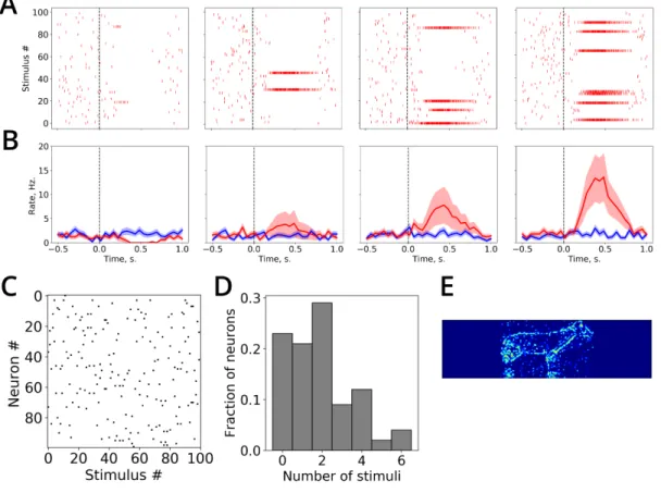
Simulation 4: Visual responses of hippocampal neurons in an image memorization task
377
This simulation was inspired by the study ofJutras and Buffalo(2010a) in which a large set of
378
novel visual stimuli was presented to monkeys on a computer screen. Neuronal activity in the
379
hippocampal formation in response to the visual stimuli was recorded. One of the results of
380
this study suggested that hippocampal neurons encode stimulus novelty in their firing rates. To
381
simulate this result, we presented to the model 100 novel stimuli randomly chosen from the dataset
382
retrieved fromhttp://www.vision.caltech.edu/Image_Datasets/Caltech101). The stimuli (resized to
383
160 × 100 pixels) were shown to the model successively in one continuous session (500ms stimulus
384
presentation time + 1000ms inter-trial interval with no stimuli) and the activities of the hippocampal
385
neurons during learning were recorded.
386
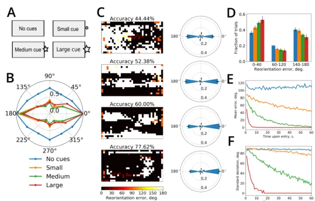
Simulation 5: Spatial reorientation
387
In this simulation of the experiment ofGouteux et al.(2001), the testing room was a rectangular
388
3D environment with area 20×10 m and wall height 6m. In the “No cues” task the only visual
389
features in the room were provided by the outlines of the walls. In the other 3 tasks, a square
390
visual cue was presented in the middle of one of the walls with the edge length equal to 1/6
391
(small cue), 1/3 (medium cue) or 1/2 (large cue) of the environment width. Each task consisted
392
of two phases, exploration and reorientation. During the exploration phase the modeled animal
393
uniformly explored the environment, as in Simulation 3. The reorientation phase composed multiple
394
trials. At the beginning of each trial, the model was placed at one of spatial locations covering
395
the environment in a uniform grid. At each of these locations, 9 successive views were taken.
396
Reorientation performance was assessed in two ways: (i) only the first view at each location was
397
used for reorientation; (ii) successive views accumulated over 60 successive positions were used for
398
reorientation.
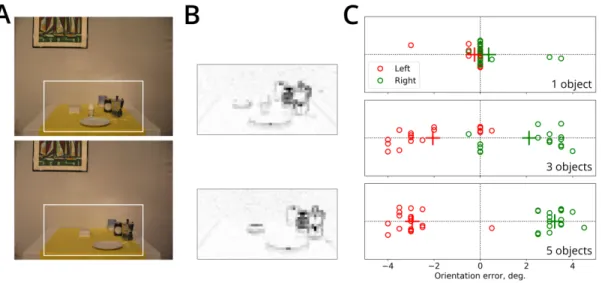
Simulation 6: Memory-based visual search
400
In this simulation we used a dataset of visual images used in the study byFiehler et al.(2014). This
401
dataset consists of 18 image sets corresponding to 18 different arrangements of the same 6 objects
402
(mug, plate, egg, jam, butter, espresso cooker). Each set includes a control image (all objects on the
403
table in their initial positions) and images in which one of the objects is missing (target object) and
404
one or more other objects displaced to the left or to the right. In the simulation we used only a
405
subset of all images in a set that included either 1, 3 or 5 of the objects mentioned above displaced
406
either to the left or to the right (referred to as “local” condition in Fiehler et al., 2014), giving rise
407
to 6 experimental conditions. In each condition, there were 18 test images of displaced objects,
408
plus the associated control images. Taking into account the distance between the animal and the
409
screen as well as the size of the image (provided byFiehler et al.(2014)), we calculated the size
410
of the image in degrees of visual field. We then determined a rectangular portion of the image
411
(30 × 15◦) that included all objects in initial and displaced positions in all images. The contents of this
412
area served as an input to the model. Thus, in this simulation the spatial resolution of the visual
413
input was higher than in the previous simulations as the visual field of the model was smaller, but
414
the size of the input network was kept the same.
415
During each simulation trial, the image of objects in initial positions was first presented to the
416
network during 2000 ms and stored by the hippocampal cells. The image of displaced objects (in
417
one of the 6 conditions above) was subsequently presented to the network for the same amount of
418
time and the orientation error was read out from the mean firing rates of the reorientation network.
419
Results
420
We first show that properties of neuronal firing along the simulated neural pathway from the
421
visual cortex to the hippocampus reflect those of biological neurons along the pathway. We then
422
demonstrate how backward projections from the hippocampus to the head direction network, can
423
explain hippocampal influence on head direction during spatial reorientation and memory-based
424
visual search.
425
Visual and parietal model neurons encode sensory representations in distinct
ref-426
erence frames
427
We start with a characterization of modeled dorsal-visual path neurons in the case when a simulated
428
animal is assumed to sit in front of a screen and is free to rotate its head (Duhamel et al., 1997;
429
Snyder et al., 1998, for simplicity, we assume that rotation occurs only in the horizontal plane). The
430
firing rate of occipito-parietal (input) neurons and the output parietal neurons as a function of the
431
allocentric position of a visual stimulus (i.e. a vertical bar moving horizontally across the visual field)
432
was measured for two different head directions (Figure 3A,B). For a neuron in the input population,
433
a change in head direction induces the corresponding change of the receptive field of the neuron,
434
since its receptive field shifts together with the head along the allocentric position axis (Figure 3C).
435
In contrast, for a parietal output neuron, a change in head direction does not influence the position
436
of its receptive field, which remains fixed in an allocentric frame (Figure 3D). To show that this is
437
also true on the population level, we measured, for all visual input cells and all parietal output cells,
438
the amount of shift in its receptive field position as a function of head direction shift, while the
439
head was rotated from −50◦to 50◦. For cells in the occipito-parietal visual area, the average linear
440
slope of the dependence is close to 1, whereas in the allocentric parietal population the average
441
slope is close to 0 (Figure 3E), meaning that these two populations encode the visual stimulus
442
in the two different reference frames: head-fixed and world-fixed. These properties of model
443
neurons reproduce well-known monkey data showing that different sub-populations of parietal
444
cortex neurons encode visual features in the two reference frames (Duhamel et al., 1997;Snyder
445
et al., 1998).
446
The receptive fields of the intermediate neurons of the coordinate transformation network
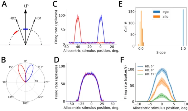
Figure 3. Properties of neurons in the coordinate-transformation network. A. A schematic representation of
the receptive field of one input visual input neuron at two head directions (HD1 and HD2). The position of the receptive field of the neuron is shown by the blue and red bar for HD1 and HD2, respectively. B. The population activity of head direction cells in the model at 20◦(HD1) and -20◦(HD2). C. Tuning curves of an input visual
neuron (±SD) for the two head directions represented in B. D. Tuning curves of an allocentric output neuron for the same head directions. E. Histograms show the distributions of the linear dependence slopes between the shift in the receptive field position and the shift in head direction, for egocentric (in blue) and allocentric (in orange) neuronal populations. F. Transformation network neurons are gain-modulated by head direction. Stimulus tuning curves of the same neuron for three different head directions are shown.
exhibit gain modulation by head direction (Figure 3F), as do monkey parietal neurons (Snyder et al.,
448
1998).The hypothesis of reference-frame conversion via gain modulation has been extensively
449
studied in both experimental and theoretical work, in the context of sensory-motor coordination
450
during vision-guided reaching (Avillac et al., 2005;Pouget and Sejnowski, 1997;Salinas and Abbott,
451
2001). While coordinate-transformation processes involved in the two cases are conceptually
452
similar, the underlying neuronal computations can differ substantially, because the former requires
453
simultaneous remapping for the whole visual field, while the latter is limited to the computation of
454
coordinates for a single target location (i.e. a representation of the point-like reaching target). This
455
difference limits the use of noise-reducing attractor-like dynamics that is an essential component
456
in point-based sensory-motor transformation models (Pouget et al., 2002), because in full-field
457
transformation the information and noise are mixed together in a single visual input stream.
458
Spatial coding using temporal accumulation of successive views
459
Because of a limited view field, at each moment in time the simulated animal can directly observe
460
only a restricted portion of visual environment (i.e. a visual snapshot, seeFigure 4A,B). That these
461
snapshot-like representations are represented in memory, has been demonstrated in a number of
462
studies showing viewpoint-dependent memory representations (Diwadkar and McNamara, 1997;
463
Christou and Bülthoff, 1999;Gaunet et al., 2001). Moreover, experimental evidence suggests that
464
visual information can be accumulated from successive snapshots during e.g. head rotation, giving
465
rise to a panoramic-like representation of the surrounding environment that can inform future
466
goal-oriented behavior (Tatler et al., 2003;Oliva et al., 2004;Golomb et al., 2011;Robertson et al.,
467
2016). A candidate neural mechanism for implementing such integration is short-term memory, i.e.
468
the ability of a neuron to sustain stimulus-related activity for a short period of time (Goldman-Rakic,
1995). In our model, this is implemented by sustained firing via prolonged NMDA receptor activation
470
(Figure 4C). Combined with STDP learning rule in the connections between the parietal output
471
neurons and the hippocampus, this mechanism ensures that a time-integrated sequence of visual
472
snapshots is stored in the synapses to hippocampal neurons. In particular, head rotation results in
473
a temporarily activated panoramic representation in the population of output parietal neurons that
474
project to CA1. STDP in these synapses ensures that these panoramic representations are stored in
475
the synapses to downstream CA1 neurons (Figure 4D).
476
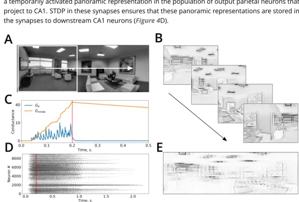
Figure 4. Temporal accumulation of successive visual snapshots in the model. A. A panoramic image of an
environment superimposed with the visual field of the simulated animal (white rectangle). The white arrow shows the direction of visual scan path. B. Several successive visual snapshots along the scan path shown in A are represented by mean firing rates of the occipito-parietal (egocentric) network. C. An example of the evolution of AMPA and NMDA receptor conductances of parieto-retrosplenial output neurons as a function of time. Stimulus onset: 𝑡 = 0, stimulus offset: 𝑡 = 200ms (red line). D. Raster plot of spiking activities of the output neurons showing short-term memory in this network. An input is presented at time 0 and is switched off at the time shown by the red vertical line. The neurons remain active after stimulus offset due NMDA-receptor mediated short-term memory. E. Synaptic weight matrix of a single hippocampal neuron after learning stores the activity of the parieto-retrosplenial output layer accumulated over several successive snapshots shown in B.
A large amount of experimental evidence suggests that many animal species encode a geometric
477
layout of the surrounding space (Cheng and Newcombe, 2005;O’Keefe and Burgess, 1996;Gouteux
478
et al., 2001;Krupic et al., 2015;Keinath et al., 2017;Bécu et al., 2019). Computational models of
479
spatial representation in rodents link this sensitivity to geometry with a postulated ability of the
480
animal to estimate distances to surrounding walls (Hartley et al., 2000) or to observe panoramic
481
visual snapshots of surrounding space (Cheung et al., 2008;Sheynikhovich et al., 2009), and rely on
482
a wide rodent visual field ( 320◦). That the width of visual field plays a role in geometric processing
483
in humans was demonstrated in the study bySturz et al.(2013), in which limiting visual field to
484
50◦impaired performance in a geometry-dependent navigation task, compared to a control group.
485
We thus studied whether activities of egocentric and allocentric neurons in the model encode
486
information about the geometry of the environment and whether snapshot accumulation over time
487
plays a role in this process.
488
To do this, we run the model to uniformly explore a square environment and we stored
popula-489
tion rate vectors of the egocentric-visual and allocentric-parietal populations at successive time
490
points during exploration. More specifically, for the egocentric population, each population vector
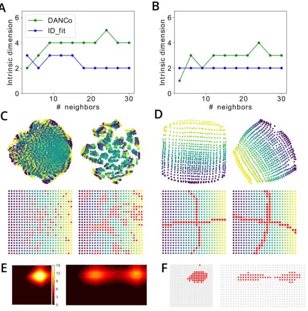
Figure 5. Representation of spatial relations by egocentric (occipito-parietal) and allocentric
(parieto-retrosplenial) visual neurons. A,B. Estimation of intrinsic dimensionality of the set of population vectors in the egocentric (A) and allocentric (B) populations by two different state-of-the-art methods (DANCo and ID_fit). C,D. Top: Projection of the population vector manifolds onto a two-dimensional plane using Isomap (left) and t-SNE (right) algorithms. Color gradient from yellow to blue corresponds to the position at which the
corresponding population vector was observed, as shown in the Bottom row. Red dots show population vectors that lie close to the principal axes of the 2D manifold of the principal space. C and D show population vectors of the egocentric and allocentric neuronal populations, respectively. E. An example of the receptive field of one hippocampal neuron after learning the environment before (left) and after (right) extension of the environment along it horizontal axis. F. For the same neuron as in E, red dots show locations in the environment where this neurons is winner in the WTA learning scheme.
corresponded to population activities evoked by the presentation of a single visual snapshot. In
con-492
trast, for the allocentric population, each population vector corresponded to a panoramic snapshot
493
obtained by accumulating several successive snapshots during head rotations (see Methods). The
494
visual information content was identical in two sets of population vectors as they were collected
495
during the same exploration trial. Population vectors in each set can be considered as data points in
496
a high-dimensional space of corresponding neural activities. These points are expected to belong to
497
a two-dimensional manifold in this space, since during exploration the model animal moves in a 2D
498
spatial plane. The analysis of the intrinsic dimensionality of both sets indeed shows that it is about
499
2 (Figure 5A,B). We then applied two different manifold visualisation techniques to see whether the