Pattern discovery allowing gaps, substitution matrices and multiple score functions

(1)

HAL Id: hal-00487245

https://hal.archives-ouvertes.fr/hal-00487245

Submitted on 28 May 2010

HAL is a multi-disciplinary open access

archive for the deposit and dissemination of

sci-entific research documents, whether they are

pub-lished or not. The documents may come from

teaching and research institutions in France or

abroad, or from public or private research centers.

L’archive ouverte pluridisciplinaire HAL, est

destinée au dépôt et à la diffusion de documents

scientifiques de niveau recherche, publiés ou non,

émanant des établissements d’enseignement et de

recherche français ou étrangers, des laboratoires

publics ou privés.

and multiple score functions

Alban Mancheron, Irena Rusu

To cite this version:

Alban Mancheron, Irena Rusu. Pattern discovery allowing gaps, substitution matrices and multiple

score functions. Workshop on Algorithms in BioInformatics (WABI), Sep 2003, Budapest, Hungary.

pp.129-145. �hal-00487245�

(2)

Substitution Matrices and Multiple Score

Functions

Alban Mancheron and Irena Rusu

I.R.I.N., Universit´e de Nantes, 2, Rue de la Houssini`ere, B.P. 92208, 44322 Nantes Cedex 3, France

{Mancheron, Rusu}@irin.univ-nantes.fr

Abstract. Pattern discovery has many applications in finding

functio-nally or structurally important regions in biological sequences (binding sites, regulatory sites, protein signatures etc.). In this paper we present a new pattern discovery algorithm, which has the following features:

- it allows to find, in exactly the same manner and without any prior specification, patterns with fixed length gaps (i.e. sequences of one or several consecutive wild-cards) and contiguous patterns;

- it allows the use of any pairwise score function, thus offering mul-tiple ways to define or to constrain the type of the searched patterns; in particular, one can use substitution matrices (PAM, BLOSUM) to compare amino acids, or exact matchings to compare nucleotides, or equivalency sets in both cases.

We describe the algorithm, compare it to other algorithms and give the results of the tests on discovering binding sites for DNA-binding proteins (ArgR, LexA, PurR, TyrR respectively) in E. coli, and promoter sites in a set of Dicot plants.

1 Introduction

In its simplest form, the pattern discovery problem can be stated as follows: given t sequences S1, S2, . . . , Ston an arbitrary alphabet, find subsequences (or

patterns) o1∈ S1, o2∈ S2, . . . , ot∈ Stsuch that o1, o2, . . . , otare similar

(accor-ding to some criterion). More complex formulations include a quorum constraint: given q, 1 ≤ q ≤ t, at least q similar patterns must be found.

The need to discover similar patterns in biological sequences is straightfor-ward (finding protein signatures, regulatory sites etc. [2]). Major difficulties are the NP-hardness of the problem, the diversity of the possible criteria of simila-rity, the possible types of patterns. All the variations in the formulation of the problem cannot be efficiently handled by the same, unique algorithm.

The consequence is that many pattern discovery algorithms have appeared during the last decade (Gibbs sampling, Consensus, Teiresias, Pratt, Meme, Mo-tif, Smile, Winnower, Splash ...). See [2] for a survey. Most of these algorithms define a quite precise model (that is, type of the searched pattern, similarity

(3)

notion, score function), even if exceptions exist (e.g., Pratt allows the use of one among five score functions). Therefore, each such algorithm treats one aspect of the pattern discovery problem, although when they are considered together these algorithms form an interesting toolkit... providing one knows to use each of the tools. Indeed, an annoying problem occurs for a biologist while using most of these algorithms: (s)he needs to have an important prior knowledge about the pattern (s)he wants to discover, in order to fix the parameters. Some algorithms do not discover patterns with gaps (Winnower [10], Projection [3]), while others need to know if gaps exist and how many are they (Smile [9], Motif [13]); some algorithms ask for the length of the searched pattern or the number of allowed errors (Smile [9], Winnower [10], Projection [3], Gibbs sampling [7]); some al-gorithms find probabilistic patterns (Gibbs Sampling [7], Meme [1], Consensus [5]); some others often return a too large number of answers (Splash [4], Teire-sias [11], Pratt [6], Smile [9]); some of them allow to use a degenerate alphabet and equivalency sets (Teiresias [11], Pratt [6]), and only one of them (Splash [4]) allows to choose a substitution matrix between amino acids or nucleic acids.

While the biologist often does not have the prior knowledge (s)he is asked for, (s)he usually has another knowledge related to the biological context: usually (s)he knows the biological significance of the common pattern (s)he is looking for (binding site, protein signature etc.); sometimes the given sequences have a particular composition (a character or family of characters appear much more often than some others); sometimes (s)he has an idea about the substitution matrix (s)he would like to use. These features could be taken into account while defining the score functions, but can we afford to propose a special algorithm for every special score function?

A way to avoid the two drawbacks cited before would be to propose an algorithm which:

i) needs a minimum prior knowledge on the type of the discovered patterns; ii) allows a large flexibility with respect to the choice of the score function, and, of course, is still able to quickly analyse the space of possible solutions in order to find the best ones. In other words, such an algorithm should be able, given a minimal description of the biological pattern, to infer a correct model (the type of the searched pattern, the similarity notion between patterns), to choose the correct score function among many possible score functions, and to (quickly) find the best patterns, that is, the ones which correspond to the searched biological patterns.

Unfortunately, when the facility of use (for a biologist) becomes a priority, and the suppleness of the algorithm (due to the need to define many types of patterns) becomes a necessity, the difficulty of the algorithmic problem grows exponentially: (1) how to deal with all the possible types of patterns, (2) what score function to use in what cases, (3) what searching procedure could be effi-cient in all these cases?

The algorithm we propose attempts to give a first (and, without a doubt, very partial) answer to these questions.

(4)

(1) Certainly, our algorithm is not able to deal with all the possible types of patterns; but it only imposes one constraint, which can be very strong or extremely weak depending on one integer parameter e. No condition on the length of the patterns, or on the number and/or the length of the gaps is needed; these features are deduced by the algorithm while analysing the input sequences and their similar regions.

(2) We use a score function f to evaluate the similarity degree between two patterns x1, x2 of the same length; f can be chosen arbitrarily, and can be

applied either to the full-length patterns x1, x2, or only to the parts of x1, x2

corresponding to significant indices. The significant indices are defined using an integer parameter Q, and are intended to identify the parts of the patterns which are common to many (at least Q%) of the input sequences.

(3) The searching procedure is supposed to discover rather general patterns, but it needs to have a minimum piece of information about the similarity notion between the patterns. There are mainly two types of similarity: the direct similarity asks that o1, o2, . . . , ot (on S1, S2, . . . , St respectively) be

similar with respect to some global notion of similarity; the indirect similarity asks that a (possibly external) pattern s exists which is similar to each of o1, o2, . . . , otwith respect to some pairwise notion of similarity. For efficiency

reasons, we chose an alternative notion of similarity, which is the indirect similarity with an internal pattern, i.e. located on one of the input sequences (unknown initially). See Remark 2 for comments on this choice.

Remark 1. The parameters e, f, Q that we introduce are needed to obtain a model (pattern type, similarity notion, score function) and to define a searching procedure, but they are not to be asked to the user (some of them could possibly be estimated by the user, and the algorithm is then able to use them, but if the parameters are not given then the algorithm has to propose default values). Remark 2. The indirect similarity with an internal pattern is less restrictive than, for instance, the direct similarity in algorithms like Pratt or Teiresias, where all the discovered patterns o1, o2, . . . , ot have to have exactly the same character

on certain positions i (every oj is, in this case, an internal pattern to which

all the others are similar). And, in general, our choice can be considered less restrictive than the direct similarity requiring the pairwise similarity of every pair (oi, oj), since we only ask for a similarity between one pattern and all the

others. Moreover, the indirect similarity with a (possibly external) pattern can be simulated using our model by adding to the t input sequences a new sequence, artificially built, which contains all the candidates (but this approach should only be used when the number of candidates is small).

Finally, notice that our algorithm is not intended to be a generalization of any of the existing algorithms. It is based on a different viewpoint, in which the priority is the flexibility of the model, in the aim to be able to adapt the model to a particular biological problem.

(5)

In Section 2 we present the algorithm and the complexity aspects. The dis-cussion of the experimental results may be found in Section 3. Further possible improvements are discussed in Section 4.

2 The algorithm

2.1 Main ideas

The algorithm is based on the following main ideas:

1.Separate the similarity notion and the score function.

That means that building similar patterns, and selecting only the interesting ones are two different things to do in two different steps. This is because we are going to define one notion of similarity, and many different score functions.

2.Overlapping patterns with overlapping occurrences form a unique pattern with a unique occurrence.

In order to speed up the treatment of the patterns, we ask the similarity notion to be defined such that if patterns x1, x2overlap on p positions and have

occurrences (that is, patterns similar with them) x′

1, x′2that overlap on the same

p positions, then the union of x′

1, x′2is an occurrence of the union of x1, x2. This

condition is similar to the ones used in alignment algorithms (BLAST, FASTA), where one needs that a pattern can be extended on the left and on the right, and still give a unique pattern (and not a set of overlapping patterns). This condition is not necessary, but is interesting from the viewpoint of the running time.

3.Use the indirect similarity with an internal pattern (say o1 on S1).

This choice allows us to define a unique search procedure for all types of patterns we consider.

4.The non-interesting positions in the internal pattern o1 (which is similar

to o2, . . . , ot) are considered as gaps.

This is already the case in some well known algorithms: in Pratt and Teire-sias a position is interesting if it contains the same character in all the similar patterns; in Gibbs sampling, a position is interesting if it contains a character whose frequency is statistically significant. In our algorithm, one can define what “interesting position” means in several different ways: occurrence of the same character in at least Q% of the patterns; or no other character but A or T in each pattern; or at least R% of A; and so on. This is a supplementary possibility offered by the algorithm, which can be refused by the user (then the searched patterns will be contiguous).

2.2 The basic notions

We consider t sequences S1, S2, . . . , St on an alphabet Σ. For simplicity, we

will assume that all the sequences have the same length n. A subsequence x of a sequence S is called a pattern. Its length |x| is its number of characters, and, for given indices (equivalently, positions) a, b ∈ {1, 2, . . . , |x|}, x[a..b] is the

(6)

(sub)pattern of x defined by the indices i, a ≤ i ≤ b. When a = b, we simply write x[a].

We assume that we have a collection of similarity sets covering Σ (either the collection of all singletons, as one often does for the DNA alphabet; or the two sets of purines and pyrimidines, as for the degenerated DNA alphabet; or equi-valency sets based on chemical/structural features; or similarity sets obtained from a substitution matrix by imposing a minimal threshold). The similarity of the characters can either be unweighted (as is usually the case for the DNA alphabet) or weighted (when the similarity sets are obtained using a substitution matrix).

Definition 1. (match, mismatch) Two patterns x, y of the same length k are said to match in position i ≤ k if x[i] and y[i] are in the same similarity set; otherwise x, y are said to mismatch in position i.

Definition 2. (similarity) Let e > 0 be an integer. Two patterns x, y are similar with respect to e if they have at most e consecutive mismatches.

From now on, we will consider that e is fixed and we will only say similar instead of similar with respect to e. Notice that the pairwise similarity notion above can be very constraining (when e is small), but can also be very weakly constraining (when e is large).

To define the indirect similarity between a set of patterns (one on each se-quence), we need to identify one special sequence among the t given sequences. Say this sequence is S1.

Definition 3. (indirect similarity, common pattern, occurrences) The patterns o1 ∈ S1, o2 ∈ S2, . . ., ot∈ St of the same length k are indirectly similar if, for

each j ∈ {1, 2, . . . , t}, o1 and oj are similar. In this case, o1 is called a common

pattern of S1, S2, . . . , St, and o1, o2, . . . , ot are its occurrences.

To define the interesting positions i of a common pattern (see 4. in subsection 2.1.), we use - in order to fix the ideas - one of the possible criteria: we ask that the character in position i in the common pattern exceed a certain threshold of matched characters in o1, o2, . . . , ot.

Definition 4. _{(consensus, gap) Let 0 ≤ Q ≤ 100 be an integer and let o}1∈ S1

of length k be a common pattern of S1, S2, . . . , Sj (1 ≤ j ≤ t) with occurrences

o1, o2, . . . , oj respectively. Denote

Ai,j= | {l , o1[i] matches ol[i], 1 ≤ l ≤ j}|, for every 1 ≤ i ≤ k

R(Q,j)= {i , Ai,j≥ Qt/100, 1 ≤ i ≤ k}.

Then the part of o1 corresponding to the indices in R(Q,j), noted o1|R(Q,j), is

the consensus with respect to Q of o1, o2, . . . , oj; the contiguous parts not in the

(7)

The use of the parameter Q allows to add (if one wishes) to the compulsory condition that o1, o2, . . . , ojhave to be similar to o1, the supplementary condition

that only the best conserved positions in o1 are to be considered as interesting

(the other positions are assimilated to wild-card positions, that is, they can be filled in with an arbitrary character). Different values of the pair (e, Q) allow to define a large range for the similar patterns and their consensus, going from a very weakly constrained notion of pairwise similarity and a very low significance of each character in the consensus, to a strongly constrained notion of similarity and a strong significance of each character in the consensus.

2.3 The main procedure

The main procedure needs a permutation π of the sequences. Without loss of generality we will describe it assuming that π is 1, 2, . . . , t. The sequences are successively processed to discover o1, o2, . . . , ot in this order such that o1 is a

maximal common pattern of S1, S2, . . . , Stwith a high score S (defined below).

Here “maximal” means with respect to extension to the left and to the right. The “high” score (as opposed to “best”) is due to the use of a heuristic to prune the search tree.

The idea of the algorithm is to consider each pattern in S1 as a possible

solution, and to successively test its similarity with patterns in S2, . . . , St. At

any step j (2 ≤ j ≤ t), either one or more occurrences of the pattern are found (and then o1 is kept), or only occurrences of some of its sub-patterns are found

(and then o1 is split in several new candidates). Each pattern is represented as

an interval of indices on the sequence where it occurs.

Definition 5. _{(offset, restriction) Let O be a set of disjoint patterns on the} sequence S1 (corresponding to a set of candidates o1), let j ∈ {1, 2, . . . , t} and

let δ ∈ {−(n − 1), . . . , n − 1} be an integer called an offset. Then the restriction of O with respect to Sj and δ is the set

O|(j, δ)={[a..b], [a..b] is a maximal subpattern of some pattern in O such that 1 ≤ a + δ ≤ b + δ ≤ n and S1[a..b] is similar to Sj[a + δ..b + δ]}.

Note that O|(j, δ) is again a set of disjoint intervals (otherwise non disjoint intervals could be merged to make a larger interval). These are the maximal parts of the intervals in O which have occurrences on Sj with respect to the

offset δ.

Each [a..b] ∈ O|(j, δ) gives a (possibly new) candidate o1 = S1[a..b] whose

occurrence on Sj is oj= Sj[a + δ..b + δ].

Every such candidate (still called o1) is evaluated using a score function,

and only the most promising of them continue to be tested in the next steps. The score function is complex, since it has to take into account both the “lo-cal” similarities between o1 and each occurrence oj (i.e. the matches and their

weights, the mismatches, the lengths of the gaps in o1 etc.) and the “global”

similarity between all the occurrences o1, o2, . . . , oj (represented by the

(8)

components: first, the similarity between o1and oj is evaluated using a Q-score;

then, a global score of o1at step j is computed based on this Q-score and on the

global score of o1 at step j − 1. The Q-score is defined below. The global score

is implicit, and is calculated by the algorithm.

Let 0 ≤ Q ≤ 100 and suppose we have a score function f defined on every pair of patterns of the same length. In order to evaluate the score of o1∈ S1and

oj ∈ Sj of length k assuming that o2 ∈ S2, . . . , oj−1 ∈ Sj−1 have already been

found, we define:

Definition 6. (Q-significant index) A Q-significant index of o1, oj is an index

i ∈ {1, . . . , k} such that either (1) i ∈ R(Q,j) and o1, oj match in position i;

or (2) i 6∈ R(Q,j) and o1, oj mismatch in position i. The set containing all the

Q-significant indices of o1, oj is noted I(Q,j).

A Q-significant index is an index that we choose to take into account when computing the Q-score between o1, oj: in case (1), the character o1[i] is

represen-tative for the characters in the same position in o1, o2, . . . , oj (since it matches

in at least Q percent of the sequences), so we have to strengthen its significance by rewarding (i.e. giving a positive value to) the match between o1[i] and oj[i];

in case (2), o1[i] is not representative for the characters in the same position in

o1, o2, . . . , oj and we have to strengthen its non-significance by penalizing (i.e.

giving a negative value to) the new mismatch.

The reward or penalization on each Q-significant index is done by the score function f , which is arbitrary but should preferably take into account the matches (with their weights) and the mismatches. As an example, it could choose to strongly reward the matches while weakly penalizing the mismatches, or the converse, depending on the type of common pattern one would like to obtain (a long pattern possibly with many gaps, or a shorter pattern with a very few gaps).

To define the Q-score, note x|I(Q,j) the word obtained from x by

concatena-ting its characters corresponding to the indices in I(Q,j).

Definition 7. (Q-score) The Q-score of o1, oj is done by

fQ(o1, oj) = f (o1|I(Q,j), oj|I(Q,j)).

The algorithm works as follows. At the beginning, the set O of candidates on S1 contains only one element, the entire sequence S1. This candidate is refined,

by comparing it to S2and building the sets of new candidates O|(2, δ2), for every

possible offset δ2 (i.e δ2 ∈ {−(n − 1), . . . , n − 1}). The most interesting (after

evaluation) of these sets are further refined by comparing each of them to S3

(with offsets δ3∈ {−(n − 1), . . . , n − 1}) and so on. A tree is built in this way,

whose root contains only one candidate (the entire sequence S1), whose internal

nodes at level L correspond to partial solutions (that is, patterns o1 on S1

which have occurrences on S2, . . . , SLand have a high value of the implicit score

function computed by the algorithm) and whose leaves contain the solutions (that is, the patterns o1 on S1 which have occurrences on S2, . . . , Stand have a

(9)

To explain and to give the main procedure, assume that we have for each node u :

- its list of offsets δ(u) = δ2δ3. . . δL(u), corresponding to the path between

the root and u in the tree (L(u) is the level of u); the offset δj signifies that if

o1= S1[a..b] then oj= Sj[a + δj..b + δj] is its occurrence on Sj with offset δj;

- its set of disjoint patterns O(u) (the current candidates on S1);

- its score score(u);

- its parent parent(u) and its (initially empty) children childp, −(n − 1) ≤

p ≤ n − 1, each of them corresponding to an offset between S1and SL(u)+1.

The procedure Choose and Refine below realizes both the branching of the tree, and its pruning. That is, it shows how to build all the children of a node u which is already in the tree, but it only keeps the most “promising” of these children. These two steps, branching and pruning, are realized simultaneously by the procedure; however, it should be noticed that, while the branching method is unique in our algorithm, the pruning method can be freely defined (according to its efficiency).

The branching of the tree is done one level at once. For each level L from 2 to t (see step 6), the list List′

contains the (already built) nodes at level L − 1, and the list List (initially empty) receives successively the most promising nodes v at level L, together with their parent u (a node from List′_{) and the corresponding}

offset δ between S1 and SL. Then, for each node u at level L − 1 (that is, in

List′_{), all its possible children v (that is, one for each offset δ) are generated and}

their set of candidates O(v) and scores score(v) are calculated (lines 10 to 13). Here comes the pruning of the tree: only the most “promising” of these nodes v will be kept in List (using an heuristics), and further developed. The objective is to find the leaves z with a high implicit score, that is, the ones for which score(z), computed successively in line 13, is high (and closed to the best score). In the present version of the procedure, we chose the simplest heuristic: we simply define an integer P and consider that a node v on level L is promising (lines 14 to 16) if it has one of the P best scores on level L. Therefore, the successively generated nodes v are successively ranged in List by decreasing order of their scores, and only the first P nodes of List are kept (line 16). These nodes are finally introduced in the tree (lines 19, 20). This simple heuristic allows to obtain, in practical situations, better results than many of the algorithms cited in Section 1 (see Section 3, where the predictive positive value and the sensibility of the results are also evaluated). Moreover, it has very low cost and provides a bound P on the number of nodes which are developed on each level of the tree. We think therefore that this heuristic represents a good compromise between the quality of the results and the running time. Further improvements, using for instance an A* approach, can and will be considered subsequently.

Finally (lines 23, 24), the sets of candidates in each leaf are considered as solutions and are ranged according to the decreasing order of their scores.

(10)

Procedure Choose and Refine

Input: a permutation π= {S1, S2, . . . , St}; integers Q (0 ≤ Q ≤ 100) and P .

Output: a set Sol of solutions o1 on S1 (decreasingly ordered w.r.t. the

final implicit score) and, for each of them, the sequence δ2δ3. . . δt.

1. begin

2. generate the root r of the tree T ; /* the tree to be built */

3. Sol:= ∅; L ← 1; /* L is the current level */

4. δ(r) ← λ; O(r) ← {[1..n]}; score(r) ← +∞; /*λ is the empty string */

5. List← {(r, 0, λ)}; List′

← List;

/* List is the decreasingly ordered list of the P most promising nodes */

6. while L < t do

7. List← ∅; L ← L + 1;

8. for each (u, a, b) ∈ List′

do

9. for δ← −(n − 1) to n − 1 do

10. generate a new node v;

11. δ(v) ← δ(u).δ; O(v) ← O(u)|(L, δ);

12. m← max {fQ(o1, oL), o1= S1[a..b], oL= SL[a + δ..b + δ]};

[a..b] ∈ O(v)

13. score(v) ← min{score(u), m};

14. if (score(v) > 0) and

(|List| < P or score(v) > minw∈Listscore(w)) then

15. insert (v, u, δ) into the ordered list List ;

16. if |List| = P + 1 then remove its last element;

17. endfor

18. endfor;

19. for each (v, u, δ) in List do

20. childδ(u) ← v; parent(v) ← u;

21. List′

← List;

22. endwhile;

23. Sol← ∪(u,a,b)∈ListO(u);

24. order the elements o1 in Sol by decreasing order of

min{score(parent(u)), fQ(o1, ot)}

(where o1∈ O(u) and ot is its occurrence on St);

25. end.

Remark 3. It can be noticed here that, if o1 is found in a leaf u, only one

occur-rence of o1is identified on each sequence Sj. In case where at least one sequence

Sj exists such that o1 has more than one occurrence on Sj, two problems can

appear: (1) the same pattern o1 is (uselessly) analysed several times at level

j + 1 and the following ones; (2) o1 counts for two or more solutions among the

P (assumed distinct) best ones we are searching for. Problem (1) can be solved by identifying, in the nodes at level L, the common candidates; this is done by fusioning the list of candidates for all the nodes of a given level. In the same way we solve problem (2) and, in order to find all the occurrences of a solution o1

on all sequences, we use a (more or less greedy) motif searching algorithm. The theoretical complexity (see Subsection 2.5) is not changed in this way.

(11)

2.4 The cycles and the complete algorithm

We call a cycle any execution of the algorithm Choose and Refine for a given permutation π (P and Q are the same for all cycles). Obviously, a cycle appro-ximates the best common patterns which are located on the reference sequence, Sπ(1). Different cycles can have different reference sequences, and can thus give

different common patterns. To find the best, say, p common patterns, indepen-dently on the sequence they are located on, at least t cycles are necessary; but they are not sufficient and it is inconceivable to perform all the t! possible cycles. Instead, we use a refining procedure (another heuristic) which tries to de-duce the p best permutations, that is, the permutations π1, π2, . . . , πp which

give the common patterns with p best scores. The main idea is to execute the procedure Choose and Refine on randomly generated permutations with refe-rence sequences respectively S1, S2, . . . , St, S1, S2, . . . and so on, until t2 cycles

are executed without modifying the p current best scores. Then the reference sequences Si1, Si2, . . . , Sipof the permutations which gave the best scores can be

fixed to obtain the first sequence of the permutations π1, π2, . . . , πp respectively.

To obtain the second sequence Sjk of the permutation πk (1 ≤ k ≤ p), the same

principle is applied to randomly generated permutations whose first sequence is Sik and second sequence is S1, S2, . . . , Sik−1, Sik+1, . . . St, S1, S2, . . . and so on.

When (t − 1)2 _{cycles have been executed without modifying the current best}

score, the second sequence of πk is fixed and, in fact, it can be noticed that it is

not worth fixing the other sequences in πk (the score will be slightly modified,

but not the common pattern). The best permutations π1, π2, . . . , πp are then

available.

The complete algorithm then consists in applying the refining procedure to approximate the p best permutations, and to return the sets Sol corresponding to these permutations. Section 3 discusses the performances of the complete algorithm on biological sequences and on randomly generated i.i.d. sequences with randomly implanted patterns.

2.5 The complexity

Our simple heuristic for pruning the tree insures that the number of developed vertices is in O(P t), so that the steps 9 to 17 are executed O(P t) times. The most expensive of them are the steps 11 and 12. They can be performed in O(n2_min{(Σ

α∈Σp2α)e, 1}) using hash tables to compute the offsets and assuming

that all Sjhave i.i.d. letters with the probability of each character α ∈ Σ denoted

pα([8], [15], [16]). Thus the running time of the procedure Choose and Refine

is in O(P tn2_min{(Σ

α∈Σp2α)e, 1}). When the letters are equiprobable, we obtain

O(P tn2_min{e|Σ|−1_{, 1}).}

The number of cycles executed by our refining procedure is limited by pt2_N

(where N is the total number of times the best scores change before the two first sequences of a permutation πk are fixed). Practically, N is always in O(t),

so that the running time of the complete algorithm, when the p best results are required, can be (practically) considered in O(pP t4_n2_min{e|Σ|−1_{, 1}). The}

(12)

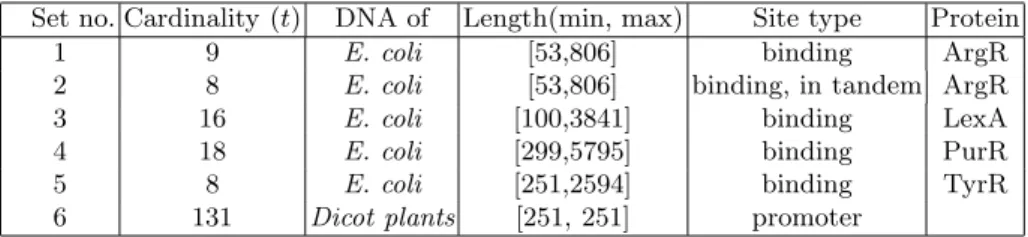
Table 1.The 6 sets of input sequences

Set no. Cardinality (t) DNA of Length(min, max) Site type Protein

1 9 E. coli [53,806] binding ArgR

2 8 E. coli [53,806] binding, in tandem ArgR

3 16 E. coli [100,3841] binding LexA

4 18 E. coli [299,5795] binding PurR

5 8 E. coli [251,2594] binding TyrR

6 131 Dicot plants [251, 251] promoter

3 Experimental results

We present here the results of the simplest implementation of the algorithm, that is, using the nucleotide alphabet {A, C, G, T } where each character is similar only to itself, and the similarity counts for 1 (while the non-similarity counts for 0). We implemented several pairwise score functions f , mainly by defining two components for each such function: a component f1 which indicates how to

reward the contiguous parts only containing matches, and a component f2which

indicates how to penalize the contiguous parts only containing mismatches. Example. For instance, if f1(a) = a√a, f2(a) = a, the value of f for x =

ACGGCT CT GGAT and y = CCGGT ACT GGCT is equal to −f2(1) + f1(3) −

f2(2) + f1(4) − f2(1) + f1(1) = 10.19 since we have mismatches in positions (1),

(5, 6), (11), and matches in positions (2, 3, 4), (7, 8, 9, 10), (12).

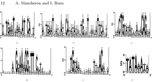
Biological sequences. To test our algorithm on DNA sequences, we used six input sets; five of them contain (experimentally confirmed) binding sites for DNA-binding proteins in E. coli and the last one contains (experimentally con-firmed) promoter sites in Dicot plants (see Table 1). For each of these sets, the sequence logo [14] of the binding (respectively promoter) sites can be seen in Fi-gure 1. Sets 1 to 5 were chosen among the 55 sets presented in [12] (whose binding sites can be found on the page http://arep.med.harvard.edu/ecoli matrices/); the only criteria of choice were the number and length of the sequences in a set (we prefered these parameters to have important values, in order to insure a large search space for our algorithm). Since the sets of sequences were not available on the indicated site, each sequence was found on GenBank by applying BLASTN on each binding site, and this is one of the reasons why we limited our tests to 5 over 55 sets of sequences. In order to enrich the type of researched patterns, we added the 6th set, whose 131 sequences (corresponding to Dicot plants) can be downloaded on http://www.softberry.com/berry.phtml.

We firstly executed our algorithm on Set 1, with different values for e and Q, and with different pairwise score functions f (including the default score function in Pratt). We learned on this first example the best values for the parameters: e = 5, Q = 70, f formed by f1(a) = f2(a) = a. With these parameters and

with P = 1, p = 1 (thus asking only for the best solution), we performed the executions on the 5 other input sets (20 executions on each set, in order to be

(13)

10

T

A

11 C T A 12 T

A

C

T

13 14 CA GT 15 T

C

T

4

G

5AG

T

6CT

A

A

CA7

T

8 G T C

A

3′ d) e) f) 1

Fig. 1.The sequence logos for the binding sites of a) ArgR; b) ArgR (binding site in

tandem); c) LexA; d) PurR; e) TyrR and for the promoter sites in f) a set of Dicot plants.

sure that different randomly generated permutations in the refining procedure do not yield different results); we found the consensi below (that means that each of the 20 executions on a given set found the same consensus). These results have to be compared with the logos, by noticing that the insignificant characters on the logos have few chances to be present in the consensus.

- For set 1, we found TGAATxAxxATxCAxxTxxxxTGxxT; the positions of the pattern on the sequences are very well found; the important length of the pattern (when compared to its logo) is explained by noticing that 8 of the 9 sequences contain the pattern in the logo twice (consecutively), while the 9th sequence contains only the beginning of the second occurrence.

- For set 2, TGAATxAxxATxCAxxTAxxxTGxxTxxxAATxCA was found; the length of the pattern is good, the locations are the good ones. The two distinct parts of the tandem are not visible here since the distance between them is simply considered as a gap in the consensus.

- For set 3, we found ACTGTATATxxAxxCAG; the length of the pattern is good, the positions on the sequences are the good ones.

- For set 4, we found GCxAxCGTTTTC; the algorithm finds very well the well conserved characters in the pattern and their positions on the sequences, but cannot find the beginning of the pattern because of the too weak similarity at this place.

- For set 5, we found TGTAAAxxAAxxTxTAC; the length of the pattern is good, the positions on the sequences are the good ones.

For these five sets, the results can be considered as being very good, when compared to the results obtained by the other pattern discovery algorithms. To make these comparisons, we restricted to the algorithms which are available via Internet (execution via a web page). We manually analysed the expected results

(14)

in each case (recall that the experimentally confirmed binding sites are known) and we fairly fixed the parameters of each algorithm, in order to insure that the solution was correctly defined. We couldn’t make comparisons in terms of real running time, since the execution conditions of these algorithms were unknown to us and some of the results were sent by email many hours later. So we limited to comparisons with concern to the quality of the results and we noticed that only Gibbs sampling and Consensus (which are probabilistic algorithms) identify the binding sites with the same precision as our algorithm. Pratt patterns obtained before refinement are shorter than the ones we find (and the ones one has to find), and they are less precise (the number of significant characters is lower); Pratt patterns obtained after refinement are really too long and very imprecise. Teiresias finds a lot of results (more than 200 for each test), and the searched result may be anywhere in the list of results; it is therefore impossible to identify it between the other results; moreover, the results are shorter than the one we find, and less precise. The too large number of results is also the drawback of Smile. Meme gives the expected result only in one case (Set 3).

- For set 6, our algorithm is the only one which identifies the pattern searched TATAAAT (good length, good significant characters), with the only problem that it finds much more locations (this is because the pattern is very frequent). The other algorithms find much longer patterns which sometimes include the searched pattern.

Conclusion. We deduce that on these examples the results of our algorithm are comparable with the best results of the best existing algorithms. The Q-significant letters are clearly found; the other ones are not indicated but they obviously could be computed by the algorithm. The identification of the biolo-gical patterns with our algorithm for P = 1, p = 1 in all these examples insures that the formal definition of the biological signals is correct; the good formal result (i.e. the one corresponding to the biological signal) is not lost in a long list of formal results (as is the case for algorithms like Teiresias and Smile). Obviously, if P, p have other values, the best result will be the same, and some other results will be added, by decreasing order of their score.

Randomly generated input sets. Our algorithm uses two heuristics (one in the procedure Choose and Refine, the other one in the refining procedure). To evaluate the performances of the algorithm (and thus of the heuristics), we eva-luated the predictive positive value (PPV) and the sensibility (S) of its results, for P = p = 1 (thus looking only for the best pattern). We executed our algorithm on 1000 arbitrarily generated input sets (at least 10 i.i.d. sequences of length at least 100 in each set) where we implanted on each sequence several randomly mutated patterns (of given scores and lengths) at randomly chosen positions. The average PPV and S values we obtained for these executions are respectively 0.95 and 0.91, which means that, on average, 95% of the pattern found by the algorithm correspond to the implanted pattern with best score, and that 91 % of the implanted pattern with best score correspond to the pattern found by the

(15)

algorithm. More precisely, that means that the found pattern is (almost) the implanted pattern with best score (it is on the same sequence, it recovers about 91 % of the indices which form the implanted pattern), but it is sometimes a little bit shifted (on the right or on the left), and one possible explanation (additionally to the one that our method is not exact) is that the insertion of the pattern with best score sometimes created in the sequence a neighboring pattern with an even better score.

4 Further improvements

We did not insisted until now on the supplementary features of some other algo-rithms with respect to ours. We already have an algorithm which is competitive with the existing ones, but it could be improved by (1) introducing a quorum q corresponding to a smaller percentage of sequences which have to contain the pattern; (2) using a better heuristic for pruning the tree (for instance, an A* approach); (3) testing the algorithm on many different biological inputs, in or-der to (non-automatically) learn the best parameters for each type of biological pattern; (4) investigating under which conditions one can improve our algorithm to use an indirect similarity with an external pattern, by introducing a supple-mentary, artificially built, sequence containing all the candidates (their number should be small enough, possibly because a pre-treatment procedure has been applied). Some of these possible ameliorations are currently in study, the other ones will be considered subsequently.

References

1. T. L. Bailey, C. Elkan: Unsupervised learning of multiple motifs in biopolymers using expectation maximization. Machine Learning, 21 (1995), 51-80.

2. B. Brejov´a, C. DiMarco, T. Vinar, S. R. Hidalgo, G. Hoguin, C. Patten: Finding

patterns in biological sequences. Tech. Rep. CS798g, University of Waterloo (2000). 3. J. Buhler, M. Tompa: Finding motifs using random projections. Proceedings of

RECOMB 2001, ACM Press (2001) 69-76.

4. A. Califano: SPLASH : Structural pattern localization analysis by sequential his-tograms. Bioinformatics 16(4) (2000) 341-357.

5. G. Hertz, G. Stormo: Identifying DNA and protein patterns with statistically sig-nificant alignments of multiple sequences. Bioinformatics 15 (1999) 563-577. 6. I. Jonassen: Efficient discovery of conserved patterns using a pattern graph.

Com-puter Applications in the Biosciences13 (1997) 509-522.

7. C. Lawrence, S. Altschul, M. Boguski, J. Liu, A. Neuwald, J. Wootton: Detecting subtle sequence signal: a Gibbs sampling strategy for multiple alignment. Science 262 (1993) 208-214.

8. D.J. Lipman, W.R. Pearson: Rapid and sensitive protein similarity search. Sciences 227 (1985) 1435-1441.

9. L. Marsan, M.-F. Sagot: Extracting structured motifs using a suffix tree. Proceed-ings of RECOMB 2000, ACM Press (2000) 210-219.

10. P. A. Pevzner, S.-H. Sze: Combinatorial approaches to finding subtle signals in DNA sequences. Proceedings of ISMB (2000) 269-278.

(16)

11. I. Rigoutsos, A. Floratos: Combinatorial pattern discovery in biological sequences: The TEIRESIAS algorithm. Bioinformatics 14(1) (1998) 55-67.

12. K. Robison, A.M. McGuire, G.M. Church: A comprehensive library of DNA-binding site matrices for 55 proteins applied to the complete Escherichia coli K-12 genome. J. Mol. Biol. 284 (1998) 241-254.

13. H.O. Smith, T. M. Annau, S. Chandrasegaran: Finding sequence motifs groups of functionally related proteins. Proc. Nat. Ac. Sci. USA 87 (1990) 826-830.

14. T.D. Schneider, R.M. Stephens: Sequence logos: a new way to display consensus sequence. Nucl. Acids Res 18 (1990) 6097-6100.

15. M. Waterman: Introduction to computational biology: maps, sequences and genomes. Chapman & Hall (2000).

16. W. Wilbur, D. Lipman: Rapid similarity searches of nucleic acid and protein data banks. Proceeding of National Academy of Science, 80 (1983) 726-730.