Discrete element modeling of the impact of granular debris flows on rigid and flexible structures

(1)

HAL Id: tel-01286617

https://tel.archives-ouvertes.fr/tel-01286617

Submitted on 11 Mar 2016

HAL is a multi-disciplinary open access archive for the deposit and dissemination of sci-entific research documents, whether they are pub-lished or not. The documents may come from teaching and research institutions in France or abroad, or from public or private research centers.

L’archive ouverte pluridisciplinaire HAL, est destinée au dépôt et à la diffusion de documents scientifiques de niveau recherche, publiés ou non, émanant des établissements d’enseignement et de recherche français ou étrangers, des laboratoires publics ou privés.

debris flows on rigid and flexible structures

Adel Albaba

To cite this version:

Adel Albaba. Discrete element modeling of the impact of granular debris flows on rigid and flexible structures. Mechanical engineering [physics.class-ph]. Université Grenoble Alpes, 2015. English. �NNT : 2015GREAI111�. �tel-01286617�

(2)

THÈSE

Pour obtenir le grade de

DOCTEUR DE L’UNIVERSITÉ GRENOBLE ALPES

Spécialité : Matériaux, Mécanique, Génie civil, Electrochimie

Arrêté ministériel : 7 août 2006

Présentée par

Adel ALBABA

Thèse dirigée par François NICOT et

codirigée par Stéphane LAMBERT et Bruno CHAREYRE préparée au sein du Laboratoire IRSTEA Grenoble

dans l'École Doctorale IMEP2

Modélisation par éléments discrets de

l’impact des laves torrentielles

granulaires sur des structures rigides

et flexibles

Thèse soutenue publiquement le 14 Décembre 2015, devant le jury composé de :

M. Jean-Yves DELENNE

Directeur de recherche, INRA Montpellier, Président du jury, Rapporteur

M. Guido GOTTARDI

Full Professor, University of Bologna, Rapporteur

M. Ali LIMAM

Professeur, INSA Lyon, Examinateur

M. François NICOT

Directeur de Recherche, IRSTEA Grenoble, Directeur de thèse

M. Stéphane LAMBERT

Ingénieur de Recherches, IRSTEA Grenoble, Co-Directeur de thèse

M. Bruno CHAREYRE

Maître de conférence (HDR), 3SR INP Grenoble, Co-encadrement de thèse

M. Thierry FAUG

(3)

(4)

Discrete element modeling of the

impact of granular debris flows

on rigid and flexible structures

(5)

Unité de Recherche Erosion Torrentielle Neige et Avalanches Domaine Universitaire, BP 76

F38402 – Saint Martin d’Hères Cedex – France [email protected]

(6)

Acknowledgement

At the end of this long journey, I would like to acknowledge the generous help and support I have received during the PhD. First, I would like to thank my thesis supervisor Prof. François Nicot for supervising and directing me during the different stages of the thesis. His commitment, passion for science and encouragement were inspirational to me. My sincere thanks go also to my co-supervisors Dr. Stéphane Lambert and Dr. Bruno Chareyre for their participation in all meetings and discussions and for their valuable contribution to the thesis development.

The thesis was funded by the People Programme (Marie Curie Actions) of the Euro-pean Unions Seventh Framework Programme FP7 under the MUMOLADE ITN project (Multiscale Modelling of Landslides and Debris Flow) grant number 289911. I would like to thank the project leader Prof. Wei Wu and the project coordinator Dr. Faqiang Qian for the perfect organization of the different schools, workshops and meeting during the project. I am also grateful to the PhD and Postdoc fellows in the project for the collaborations and discussions.

I would also like to thank my colleagues in both laboratories IRSTEA and L3SR in Grenoble for their scientific collaboration and suggestions during the internal meetings and workshops. Special thanks for Raphael Murin my office mate for helping me with different aspects of numerical coding, François Kneib for helping me with YADE open source code and its different features, and Dr. Thierry Faug for his suggestions concern-ing the granular flow impact on rigid walls.

(7)

Many contributions from engineers and researchers working with the industry of natural hazard protection were greatly supportive. These include the ones from Nicollas Villard (GTS) whose presence in many committee meetings greatly highlighted the prac-tical aspects of the numerical model of flexible barriers. Discussions with Dr. Corrina Wendler (GeoBrugg) during MuMoLaDe’s meetings and workshops were of great help, thanks to her in-depth knowledge of flexible debris flow barriers.

Finally, I would like to thank my family and friends for their unlimited support during these years, especially my wife for standing beside me throughout the thesis. A lot of work I carried out was on weekends, nights, while on vacation, and other times inconvenient for her, so I am grateful for her patience and sacrifice.

(8)

Abstract

Natural hazards such as debris flows are real threat to the urbanization of mountainous areas. Local communities and infrastructures can be exposed to large impact forces in extreme debris events. Mitigation of such threats requires, along other measures, the estimation of the impact of such flows on protection structures (rigid walls and flexible barriers). In this thesis, Discrete Element Method (DEM) is used to model the granular flow, the rigid walls and flexible barriers.

First, a dry granular flow made of non-spherical particles flowing in inclined plane is modeled using a visco-elastic contact law with Mohr-Coulomb failure criterion. Experi-mental data from the literature is used to calibrate and validate the model. The model is calibrated based on the shape of the particle, the flow thickness and the final shape of the deposit on the wall. Validation procedure is based on the impact on a rigid wall divided into six segments. The main contribution of total normal force applied on the wall is found to be due to the dynamic component. On the micro-scale, development of force chains is believed to cause heterogeneous distribution of normal force on each part of the wall, for multiple same-test conditions.

Next, a flexible barrier is modeled using cylindrical elements. The impact on the barrier is modeled using the same flow model used for wall-impact problem. The use of energy dissipators is found to be essential for minimizing the impact force on the barrier, and thus controlling the force applied on the lateral anchors.

By comparing a rigid wall and a flexible barrier for the same flow, we found that the rigid wall is exposed to higher impact force, due its high global stiffness compared with the flexible barrier. Next, different simulations are carried out to recommend design guidelines for the flexible barrier. It is found that using a mesh size as large as D90 of the

(9)

flow is acceptable in terms of mass retaining capacity. In addition, not fixing the bottom cable of flexible barriers might lead to the total loss of its retaining capacity in extreme events.

Keywords:

Discrete Element Method, Debris flows, Rigid Walls, Flexible Barriers, Protection Struc-tures, Force Chains, Granular Flows

(10)

Résumé

Les risques naturels tels que les laves torrentielles constituent des menaces réelles pour les zones urbanisées de montagne. Les bâtiments et infrastructures peuvent être exposés à de grandes forces d’impact en cas d’évènement extrême. La réduction de cette menace, par des ouvrages de protection, impose de quantifier l’impact de ces écoulements sur les structures, qu’elles soient flexibles ou rigides.

Tout d’abord, un écoulement granulaire sec, composé de particules non-sphériques glissant sur un plan incliné, est modélisé en utilisant une loi de contact visco-élastique avec critère de rupture de Mohr-Coulomb. Des données expérimentales de la littérature ont été utilisé pour calibrer et valider le modèle. À cette fin, la forme de la particule, l’épaisseur de l’écoulement et la forme finale du dépôt sur le mur sont considerés. La validation est basée sur l’impact sur un mur rigide divisé en six segments. La principale contribution de la force totale normale appliquée sur le mur est due à la composante dynamiques. La distribution hétérogène de la force normale sur chaque partie du mur est due au développement des chaînes de force différent pour chaque arrangement des particules.

Ensuite, un filet est modélisé en utilisant des éléments cylindriques. L’impact sur le filet est modélisé en utilisant le même modèle d’écoulement que précédemment. Le rôle des dissipateurs d’énergie apparaît essentiel pour réduire la force d’impact sur le filet et limiter la force appliquée sur les points d’ancrage latéraux.

Pour la première fois, des simulations montrent que pour un même écoulement granulaire la force d’impact est plus élevée pour un obstacle rigide, avec une différence de 50% par rapport à un obstacle flexible. les simulations permettent de définir quelques recommandation pour le dimensionnement des filets. Il est constaté que l’utilisation

(11)

d’un maillage de filet plus petit que D90 de l’écoulement est acceptable en termes de capacité à retenir les matériaux en écoulement. En plus, si le câble en bas du filet n’est pas fixé, le filet pourrait perdre totalement sa capacité de retenue.

Mots clés:

Modélisation par éléments discrets, Laves torrentielles granulaires, Écoulement gran-ulaire sur plan incliné, Mur rigide, Structure de protection, filet de protection, Lignes directrices pour le design des filets

(12)

Abbreviations

Ac

Reference surface area of a cylindrical element bo Bottom opening of a flexible barrier

D50 Value of the particle diameter at 50% in the cumulative_distribution DEM Discrete Element Method

des1

A flexible barrier where the lateral cables are connected to energy dissipators which are then connected to lat-eral anchors

des2 A flexible barrier where the lateral cables are directly_{connected to the lateral anchors}

DG Design guidelines

D_lc Diameter of lateral cables Dmc Diameter of main cables Dn Diameter of the net elements Dr Diameter of sliding rings

E Elastic modulus

E_b Bending modulus

Ec Elastic modulus of the cylindrical element

ED Energy Dissipator

E_kin Total kinetic energy En Elastic modulus of the net Erot Rotational kinetic energy

(13)

f bG A flexible barrier positioned in a direction parallel to the gravity vector

f bN A flexible barrier positioned in a direction normal to the channel base

f bNo Flexible barrier without energy dissipators Fa

Mean values of forces on the two anchors located at the extremities of a given main cable

F_d Dynamic component of the total normal force

F_dead Force applied by dead particles on a protection struc-ture

F_ED₋_els Elastic limit of the forces in the energy dissipators in which afterwards it starts deforming

FEM Finite Element Method

Fg Gravitational component of the total normal force F_i Resultant force applied on particle i

Fint Interaction force

Fmov

Force applied by moving particles on a protection struc-ture

Fn Normal contact force

Fr Froude number

Fres Residual force at the end of the impact Ft Tangential contact force

Ftotn Total normal force Ftott Total tangential force

G Weight of the dead zone

G Gravity vector

g Gravity acceleration

Gtw Shear modulus for the twisting moment

H Filling height of debris flows behind protection struc-tures

h Flow depth

(14)

xi h_cl Flow centerline

Hdead Height of the dead zone behind a protection structure H_{f b} Flexible barrier height

h_i Distance between the centroid of segment i of the wall and the chute base

Hmov

Height of the moving particles that are interacting with a protection structure

h_particle Particle height

Hw Height of the rigid wall I_b Bending moment of inertia I_i Moment of inertia of particle i Itw Polar moment of inertia

K Empirical factor related to the lateral earth pressure coefficient

k_b Bending stiffness

k_i Stiffness of a spring connecting two particles kn Normal stiffness of the contact

kt Tangential stiffness of the contact ktw Twisting stiffness

Lc Length of a cylindrical element l_ch Channel length

Mb Bending moment

m_dz Dead zone mass at a given time

M_i Resultant moment applied on particle i mi Mass of particle i

MPM Material Point Method

Mt Twisting moment

mtot Total mass of the granular flow

np Number of particles in the simulation nv Number of particles in a targeted volume PIV Particle image velocimetry

(15)

r Radius of a particle

Rc Radius of the cylindrical element R_i Radius of particle i

rigW Rigid wall

R1 Base reaction

R2 Wall reaction

R1t Sum of tangential contact forces between particles and_{the chute base} R1n Sum of normal contact forces between particles and_{the chute base} R2t Sum of tangential contact forces between particles and_{the wall} R2n Sum of normal contact forces between particles and_{the wall} SDEC Spherical Discrete Element Code

Sm Mesh size of the net

SPH Smoothed-Particle Hydrodynamics Svir Virtual sphere of the cylindrical element tc Collision duration

un

Normal displacement (overlapping distance between two particles)

ut Tangential displacement

Ux Average flowing velocity in the direction of the flow Uz

Average flowing velocity in the direction perpendicu-lar to the flow

˙u(0) Relative velocity before the collision ˙u(t0_c) Relative velocity after the collision

v Impact speed

v Depth-averaged velocity of the flow Vmax

Velocity of the flow at the time of maximum total nor-mal impact force on the wall, measured for particles lying in distances from 40 to 50 cm away from the wall

(16)

xiii Vs Volume of a single D50-particle of the granular sample

Vt Total volume of the granular sample

w_ch Channel width

W_{f b} Flexible barrier width

WP Work Package

YADE Yet Another Dynamic Engine ˙ω_i Angular velocity of particle i ¨

ωi Angular acceleration of particle i x_i Position of particle i

˙x_i Rotational velocity of particle i ¨x_i Rotational acceleration of particle i γs Specific weight of gravel particles γn Normal visco-elastic coefficient

γt Specific weight of the granular sample εn Normal restitution coefficient

λ Empirical factor related to the hydrodynamic pressure

∆t Time step

α Inclination angle of the base of a channel p_dyn Hydrodynamic pressure

pstat Hydrostatic pressure

ρ Flow density

φ Microscopic friction angle

θFtot Orientation of the total force applied by the flow θ_{f b} Angle between the initial position of the flexible barrier

and the gravity vector θrc Ring-cable friction angle

δ1 Angle of friction between the base and the dead mass δ2 Angle of friction between the wall and the dead mass δrc

Friction angle between the main cables and the sliding rings

(17)

δED

Mean value of deformation of the two energy dissipa-tors installed at the ends of a given main cable

δED−brk

Maximum allowable deformation of the energy dissi-pators

Ωb 12

Bending component of the relative rotation between two spheres

Ωtw 12

Twisting component of the relative rotation between two spheres

σ_nel Elastic tensile limit σ_sel Elastic shear limit

(18)

List of Figures

1.1 Areas with landslide hazards, based on opinions of national experts of European Geological Surveys ((afterESPON,2005), origin of data: EuroGeographics associa-tion for the administrative boundaries) . . . 3 1.2 The different stages of landslide and debris flow, divided into four work packages

within MuMoLaDe project . . . 5 2.1 The six investigated configurations of granular flows: (a) plane shear, (b) annular

shear, (c) vertical-chute flows, (d) inclined plane, (e) heap flow, (f) rotating drum (afterMiDi,2004) . . . 12 2.2 Profiles of the solid fraction and the velocity in the direction of the flow, as a

function of the distance from the channel base: (a) 2D simulation, (b) 3D simulation (afterSilbert et al.,2001) . . . 14 2.3 A triangular dead zone is formed upstream of a rigid wall in which moving

particles overflow it. The white horizontal arrow indicates the incoming flow direction which is made of glass beads (afterCaccamo et al.,2012) . . . 16 2.4 Schematic representation of the different parts of flexible debris flow barriers . . . 18 2.5 Snapshots at different time of falling boulder intercepted by a flexible barrier: FEM

Numerical simulation (right) compared with photograms (left) (after Gentilini et al.,2012) . . . 21 2.6 DEM modeling of a net using remote interactions (afterBertrand et al.,2012) . . . 22 2.7 Calculation cycle in DEM . . . 26 3.1 (a) Shape of gravel particles, (b) Grain size distribution of the particles (afterJiang

and Towhata,2013) . . . 31 3.2 Rigid wall division from the bottom to the top (adapted fromJiang and Towhata,

2013) . . . 32 3.3 Normal and tangential interaction forces of the contact law used in the model . . . 35 3.4 Particle shapes tested in the simulation: a clump and a simple sphere . . . 36 3.5 Static equilibrium of the dead zone accumulated behind the wall . . . 38 3.6 Schematic representation of three different granular deposits (of same volume)

showing the indirect relation between the final shape of the deposit and the residual force applied on the 6th segment of the wall . . . 39 3.7 Variation of normal force on part 6 of the wall with time for clumps and spheres

(test L44-H15-α40◦_{) . . . 40}

3.8 Ratio of rotational energy to total kinetic energy for clumps and spheres (test L44-H15-α40◦_{) . . . 41}

3.9 Snapshots of the experiment showing frictional and collisional regimes of the flow, top: before the impact, bottom: after the impact (afterJiang and Towhata,2013) . . 42

(23)

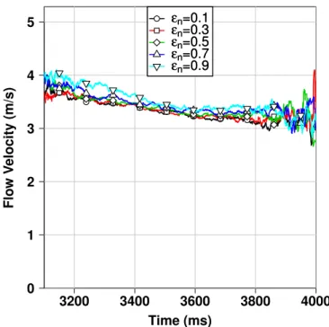
3.10 Variation of average flow thickness (flow centerline) with time using different normal restitution coefficient values (test L44-H15-α40◦_{) . . . 43}

3.11 Variation of normal force on the sixth segment of the wall with time using different normal restitution coefficient values (test L44-H15-α40◦_{) . . . 44}

3.12 Variation of average particles velocity with time, for particles in the upper half of the flow (test L44-H15-α40◦_{) . . . 45}

3.13 Cumulative frequency of particles height measured from the center (test

L44-H15-α40◦) . . . 46

3.14 Variation of particles velocity with heights (test L44-H15-α40◦_{) . . . 46}

3.15 Snapshots of the 3D view of the evolution of the calibrated flow through time (test L44-H15-α40◦_{), along with the evolution of dead particles (colored in white): (a) at}

time = 2300 ms, (b) at time = 2793 ms, (c) at time = 3583, (d) at time = 4400 ms . . . 47 3.16 Time evolution of the normal impact force on the bottom segment of the wall: raw

data and spline-treated data . . . 48 3.17 Time history of normal force variation: experiment (after Jiang and Towhata,

2013) (left) and model (right): (a) test L34-H15-α45◦_{(b) test L44-H15-α40}◦ _{(c) test}

L44-H20-α40◦ _{. . . 50}

3.18 Time history of total normal force and bending moment, test L44-H15-α40◦_:

nu-merical model and experiment (data fromJiang and Towhata,2013) . . . 52 3.19 Variation of normal residual force with wall’s height for 5 tests carried out under

the same initial conditions (test L44-H15-α40◦_{) . . . 54}

3.20 The final deposit shape for five tests that have the same initial conditions (test L44-H15-α40◦_{) . . . 54}

3.21 Residual normal contact forces between segments 1 and 2 of the wall and particles deposited on them, top: test 4, bottom: test 5 . . . 55 3.22 Time history of the evolution of total normal force and bending moment (at the

toe) for five tests that have the same initial conditions (test L44-H15-α40◦_{): (a) Total}

normal force, (b) Total bending moment . . . 57 3.23 Variation of the total normal force with time, for different ratios of Hw/d50 . . . 58

3.24 Relationship between the amplitude of the total normal force and the ratio of Hw/d50 59

3.25 Variation of total normal force components with time (test L44-H15-α40◦_{) . . . 61}

4.1 Main components of flexible debris flow barriers (a) Schematic representation, (b) YADE model . . . 66 4.2 A schematic representation of the sliding rings arrangement: (a) front view of the

net, ring and main cables, (b) cross section of the ring . . . 68 4.3 Energy dissipators: (a) Before the impact, (b) At the end of the impact (after

Bertrand et al.,2012), (c) The force:displacement response of the energy dissipators considered in our DEM model . . . 70 4.4 A sample of two connected cylindrical elements with two nodes at the ends of

each cylinder . . . 72 4.5 A representation of the sphere-cylinder interaction showing the virtual sphere of a

cylinder at the contact point . . . 74 4.6 The distance vector between two non-intersecting cylinders (adapted from

Effeind-zourou et al.,2016) . . . 76 4.7 Experimental punching test (a) cone punching element (b) rounded-concrete

punching element (afterBonati and Galimberti,2004) . . . 78 4.8 Net punching results comparison between the experiment (data fromBonati and

Galimberti,2004) and the model . . . 79 4.9 The simulated net punching test in the numerical model with DEM . . . 79

(24)

LIST OF FIGURES xxi 4.10 The evolution with time of the average deformation of each two energy dissipators

at the same cable, for different values of friction between the sliding rings and main cables . . . 81 4.11 The evolution with time of the maximum extension of main cables in the direction

of the flow, for different values of friction between the sliding rings and main cables 82 4.12 The evolution with time of the average force on each two anchors at the same cable,

for different values of friction between the sliding rings and main cables . . . 82 4.13 The evolution with time of the average flow velocity component for two cases: a

flexible barrier without energy dissipators (fbNo) and a flexible barrier with energy dissipators (fbEd): (a) in the direction of the flow, (b) perpendicular to the channel base . . . 86 4.14 The evolution with time of the total force applied on the barrier for two cases: a

flexible barrier without energy dissipators (fbNo) and a flexible barrier with energy dissipators (fbEd) . . . 87 4.15 The evolution with time of the direction of the total force vector with respect to the

channel base for two cases: a flexible barrier without energy dissipators (fbNo) and a flexible barrier with energy dissipators (fbEd). Inset: schematic representation of the total force vector direction with respect to the initial position of the barrier and the channel bed . . . 88 4.16 A side view snapshot of the the flowing material impacting the barrier showing

dead zone (in white) and moving particles (in grey) overflowing it . . . 89 4.17 The evolution with time of the dead zone mass for two cases: a flexible barrier

without energy dissipators (fbNo) and a flexible barrier with energy dissipators (fbEd) . . . 90 4.18 Snapshots of the granular flow impact on the flexible barrier with energy

dis-sipators (fbEd) showing the lateral escaping windows: (a) top view, (b) front view . . . 91 4.19 The evolution with time of the internal forces in main cables for two cases: a

flexible barrier without energy dissipators (fbNo) and a flexible barrier with energy dissipators (fbEd) . . . 93 4.20 The evolution with time of the average deformation of each two energy dissipators

at the same cable, for a flexible barrier with energy dissipators (fbEd) . . . 94 4.21 The evolution with time of the maximum extension of main cables in the direction

of the flow for two cases: a flexible barrier without energy dissipators (fbNo) and a flexible barrier with energy dissipators (fbEd) . . . 94 4.22 The evolution with time of the average force on each two anchors at the same cable,

for two cases: a flexible barrier without energy dissipators (fbNo) and a flexible barrier with energy dissipators (fbEd) . . . 95 4.23 Tensile forces in cylinders forming main cables: (a) flexible barrier without energy

dissipators (fbNo), (b) flexible barrier with energy dissipators (fbEd) . . . 97 4.24 Tensile forces in cylinders forming net elements: (a) flexible barrier without energy

dissipators (fbNo), (b) flexible barrier with energy dissipators (fbEd) . . . 98 4.25 Tensile forces larger than 50 kN in cylinders forming main cables and net elements:

(a) flexible barrier without energy dissipators (fbNo), (b) flexible barrier with energy dissipators (fbEd) . . . 101 4.26 snapshot of the top left part of the barrier: (a) flexible barrier without energy

dissipators (fbNo), (b) flexible barrier with energy dissipators (fbEd) . . . 102 4.27 The evolution with time of the average flow velocity for different values of channel

inclination angle: (a) in the direction of the flow, (b) perpendicular to the channel base . . . 104

(25)

4.28 The evolution with time of the total force applied on the barrier, for different values of channel inclination angle . . . 105 4.29 The evolution with time of the dead zone mass, for different values of channel

inclination angle . . . 106 4.30 The maximum total force and maximum average flowing velocity in the direction

of the flow, for different values of channel inclination angle . . . 107 4.31 The relation between the evolution of the total force with the evolution of the dead

zone mass, for different values of channel inclination angle . . . 108 4.32 Force per unit width measured on a wall impacted by a granular flow (made of

beads) versus time t for three slope inclinations: α =21◦, 27◦ and 33◦ (afterFaug et al.,2011) . . . 109 4.33 A schematic representation of the inclination of the flexible barrier with respect to

the gravity vector . . . 110 4.34 The evolution with time of the average flow velocity component in the direction

of the flow for different inclination angle of the barrier with respect to the gravity vector . . . 111 4.35 The evolution with time of the dead zone mass for different inclination angle of

the barrier with respect to the gravity vector . . . 111 4.36 The evolution with time of the average deformation of the two energy dissipators

at cables 3 and 4, for different inclination angle of the barrier with respect to the gravity vector . . . 112 5.1 Hydrostatic and hydrodynamic pressures applied on a barrier impacted by debris

flow (afterVolkwein,2014) . . . 118 5.2 Pressures applied on the wall: (a) Dead and moving parts of the flow, (b) Pressures

fromVolkwein(2014), (c) The equivalent pressures considered for comparison with DEM results . . . 120 5.3 Evolution of forces applied on a barrier by a granular flow calculated by the DEM

model and Volkwein load-estimation guidelines: (a) Force transmitted through the dead zone, (b) Force transmitted through the moving particles . . . 121 5.4 Side view, top view, and velocity map for different time points of a dry granular

flow impacting a rigid wall (afterJiang and Towhata,2013) . . . 123 5.5 Snapshots at given times of the velocity map of particles that that lie in the middle

of the channel . . . 125 5.6 Average flow velocity component for three structures: a flexible barrier without

energy dissipators (fbNo) and a flexible barrier with energy dissipators (fbEd) and a rigid wall (rigW): (a) in the direction of the flow, (b) perpendicular to the channel base . . . 126 5.7 Evolution of the total force applied by the flow, for three structures: a flexible

bar-rier without energy dissipators (fbNo) and a flexible barbar-rier with energy dissipators (fbEd) and a rigid wall (rigW) . . . 127 5.8 Evolution of dead zone mass, for three structures: a flexible barrier without energy

dissipators (fbNo) and a flexible barrier with energy dissipators (fbEd) and a rigid wall (rigW) . . . 129 5.9 Evolution of overflowing percentage for different values of bottom openings of

the barrier . . . 131 5.10 Evolution of maximum vertical displacement of the bottom cable with the

over-flowing percentage for different values of bottom openings of the barrier . . . 131 5.11 Evolution of overflowing percentage for different values of mesh size of the net . . 132

(26)

LIST OF FIGURES xxiii 5.12 Evolution of average flowing velocity in x-direction for two cases: a flexible barrier

parallel to gravity vector (fbG) and a flexible barrier normal to the channel base (fbN)134 5.13 Evolution of total force applied on the barrier for two cases: a flexible barrier

parallel to gravity vector (fbG) and a flexible barrier normal to channel base (fbN) 135 5.14 Evolution of dead zone mass behind the barrier for two cases: a flexible barrier

parallel to gravity vector (fbG) and a flexible barrier normal to channel base (fbN) 135 5.15 Side view of the final retained mass of a flexible barrier normal to channel base (fbN)136 5.16 Evolution of deformation of energy dissipators installed on cables 3, 4 and 5 for

two cases: a flexible barrier parallel to gravity vector (fbG) and a flexible barrier normal to channel base (fbN) . . . 137 5.17 Schematic representation of two technologies for connecting the lateral cables: (a)

lateral cables connected to energy dissipators (des1), (b) lateral cables connected

directly to the anchors (des2) . . . 138

5.18 Evolution of total force applied on barriers with two different configurations of the lateral cables: lateral cables connected to energy dissipators (des1) and lateral

cables connected directly to the anchors (des2) . . . 138

5.19 Evolution of the dead zone mass for two different configurations of the lateral cables: lateral cables connected to energy dissipators (des1) and lateral cables

connected directly to the anchors (des2) . . . 139

5.20 Evolution of the deformation of energy dissipators for two different configurations of the lateral cables: lateral cables connected to energy dissipators (des1) and lateral

5.21 Evolution of forces applied on the anchors for two different configurations of the lateral cables: lateral cables connected to energy dissipators (des1) and lateral

5.22 Snapshot at the end of the impact event showing the extra length of the net as a solution to optimize the retaining capacity . . . 142

(27)

(28)

List of Tables

(29)

(30)

Chapter 1 General Introduction

1.1 Landslides and debris flows: a threat to urbanization

Geohazards such as land slides and debris flows present a serious threat to communities and infrastructures, especially in mountainous areas. Landslides are usually triggered by heavy rainfalls which cause slope instabilities. Such instabilities, under the effect of gravity, cause landslides either partially or fully saturated which lead to the development of debris flows. As they flow down slopes, debris flows grow in volume due to the entertainment of the bed and catch the large blocks and trees along their way.

Landslides cause millions of dollars in damage and thousands of deaths and injuries each year as well as loss of productive land (Hervás,2003). They are present all over the world, especially in Europe, east Asia and the coastal parts of the Americas. In Europe, in particular, great efforts have been given over the decades to tackle this problem. How-ever, until now, several European countries are still exposed to high hazard of landslides (Fig 1.1) which cause disasters resulting in casualties and injuries and also huge damage to urbanized areas.

In Sarno (Italy), in 1998, large number of mudflows took place in the area following a heavy long-lasting rainfalls which triggered 150 landslides in 10 hours. Their destructive nature was due to their high flowing velocities (up to 14 m/s) and their total volume (several hundreds m3_{). The event caused 160 fatalities in the affected municipalities. The} total cost of the damage was estimated to be around 35 million euros including destroyed houses and infrastructure (Hervás,2003). Other examples include Stoze landslide and the Predelica torrent debris flow (2000, Slovenia), San Miguel Island landslides (1997, Portugal), Vagnharad landslide (1997, Sweden) and Ionian coast landslides and debris flows (2009, Italy).

In response to these catastrophic events, researchers have developed theories and carried out physical and numerical modeling of landslides and debris flows in order to analyze their behavior and predict their occurrence. In an effort to deepen the un-derstanding of debris flows, the European project MuMoLaDe started in 2012 to study landslides and debris flows from both experimental and numerical aspects in addition to modeling and design of debris flow mitigation structures.

(32)

1.1 Landslides and debris flows: a threat to urbanization 3

Figure 1.1:Areas with landslide hazards, based on opinions of national experts of European Geo-logical Surveys ((afterESPON,2005), origin of data: EuroGeographics association for the administrative boundaries)

(33)

1.2 Research framework (MuMoLaDe Project)

MuMoLaDe (Multiscale Modelling of Landslides and Debris Flows) is a European project within the framework of Marie Curie ITN (Initial Training Networks). It groups 13 full partners and 8 associated partners in a consortium including research institutes, universi-ties, contractors, manufacturers and software developers. The overall aim of the project, in addition to the scientific outcome, is to provide high quality training for a group of young researchers. Such training will enable them to work in multidisciplinary research of natural hazards.

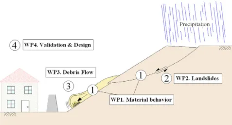
MuMoLaDe deals with the numerical and physical modeling of landslides and debris flows. 14 PhD students and 2 postdocs have been selected to study these phenomena. Their work covers the different stages of debris flow and landslides (Fig 1.2) by four work packages (WP):

• WP1: experimental testing to understand the material behavior (e.g. triaxial tests of soil samples)

• WP2: numerical (Finite element analysis) and physical modeling (centrifuge model tests) of slope stability failure to analyze the landslide initiation

• WP3: numerical (Finite Element and Discrete Element simulations) and physical modeling (rotating drum and inclined flume) of the evolution of debris flow in a channel

• WP4: the validation and design of structures protecting communities and infras-tructure (numerical Discrete Element modeling)

The role of the this thesis, within the MuMoLaDe project, lies within work packages 3 and 4. This is because part of the work of this thesis deals with the evolution of channelized debris flow (WP3) while the other half deals with the impact and design of protection structures. This is achieved through the collaboration with other PhD students in the work package and also with other members of MuMoLaDe consortium.

(34)

1.3 Thesis objectives 5

Figure 1.2:The different stages of landslide and debris flow, divided into four work packages within MuMoLaDe project

1.3 Thesis objectives

Debris flows can be classified, along other classifications, into two types: stony debris flows (coarse-grained debris flow) and muddy debris flows (fine-grained debris flow)

(Takahashi,2007). This thesis is concerned with the first type, in which stress is

domi-nated by particle collision. This granular stony-type debris flow is approximated in the DEM model as a dry granular flow.

The thesis, based on numerical simulations using Discrete Element Method (DEM), has been divided into three stages. Each stage contributes to one year of the thesis three-years period. These stages are the following:

• Modeling of dry granular flow in inclined plane impacting a rigid wall. The objective of this part is to calibrate and validate a DEM model against experimental data of dry granular flow composed of gravel particles impacting a rigid wall. As a result, we will be able to account for debris-structure impact forces and estimate the micromechanical behavior of particles during the impact process.

• Modeling the different components of flexible barriers. The objective of this part is to be able to account for the behavior of different components of flexible barriers using DEM-based model. This is to investigate the behavior of flexible barriers when impacted by the dry granular flow model calibrated/validated in the first part.

(35)

• Parametric analysis, design guidelines and best practice. The objective of this part is provide recommendations for engineers concerning the best practice in designing flexible barriers, how to optimize retaining capacity and reduce the forces applied in the different components of flexible barriers.

1.4 Thesis structure

This Thesis is divided into five chapters: the first chapter has presented a general in-troduction of the thesis. In the second chapter, the state of the art concerning granular debris flows and protection structures is presented. Special attention is given to the physical and numerical modeling of granular flows in inclined planes. Moreover, the different numerical models proposed in the literature for modeling flexible barriers (for both rockfalls and debris flows) are presented. In addition, the Discrete Element Method (DEM) is presented showing its interaction calculating cycle and time step calculation.

In the third chapter, the modeling of a dry granular flow in inclined flume is presented. The experimental data used for model calibration and validation is detailed coupled with the effect of the shape of the particles on the results. Results concerning the impact force applied on a rigid wall are analyzed. Special attention is given to the evolution of the dead zone mass which controls the gravitational part of the total force on the wall. Afterwards, microstructural analysis are carried out to investigate the reason behind the presence of microstructural heterogeneities in the impact results. The effect of the size of the particles on the total normal force signal is also analyzed.

In the fourth chapter, the impact of granular flows on flexible barriers is investigated. First, the DEM-based model used to simulate the different components of flexible bar-riers is presented. Afterwards, the different components forming the flexible barbar-riers are described along with their validation. Then, full scale simulations are carried out to present the model’s prediction of the impact behavior and the importance of the presence of energy dissipators for flexible barriers. Results concerning total impact force, forces in the anchors and load transmission within the barrier are comparatively analyzed. Parametric analysis are carried out at the end demonstrating the effect of the inclination angle of the bed on the impact force applied on the barrier and the rate of dead zone formation.

(36)

1.4 Thesis structure 7 In the fifth chapter, impact estimation models used by designers of debris flow protection structures are compared with the DEM model in terms of the impact force applied by the flow. Next, the difference is highlighted between rigid and flexible structures when impacted by the same granular flow. Afterwards, the dimensioning of flexible barriers is investigated in terms of the net mesh size and the bottom opening of the barrier. Next, the initial configuration of flexible barriers are investigated. Finally, conclusions and perspectives are globally drawn from the thesis outcomes.

(37)

(38)

Chapter 2 State of the art

2.1 Introduction . . . 10 2.2 Debris flows . . . 10 2.2.1 Physical modeling of granular flows . . . 11 2.2.2 Numerical modeling of granular flows in inclined planes . . . 13 2.3 Rigid walls for debris flow hazard mitigation . . . 14 2.3.1 Physical modeling of granular flows impact on rigid walls . . . . 15 2.3.2 Numerical modeling of granular flows impact on rigid walls . . . 17 2.4 Flexible barriers for debris flows retention . . . 18 2.4.1 Flexible barriers: Rockfalls Vs. Debris flows . . . 19 2.4.2 Numerical and physical modeling of flexible barriers . . . 20 2.5 Debris flow impact models for engineers and design guidelines . . . . 23 2.5.1 Debris flow impact models for engineering purpose . . . 23 2.5.2 Design guideliens of flexible debris flow mitigation barriers . . . 24 2.6 Discrete Element Method for modeling granular assemblies . . . 25 2.6.1 Calculation cycle in DEM . . . 25 2.6.2 Critical time step in YADE . . . 27 2.6.3 YADE-DEM code . . . 28

(39)

2.1 Introduction

In this chapter, the previous works on granular flows and protection structures are presented. For granular flows, special attentions is given to numerical and physical modeling of granular flows in inclined planes. Then, experimental and numerical modeling of the impact of granular flows on rigid walls is highlighted. Afterwards, different numerical schemes proposed for modeling flexible barriers are presented, showing the difference between the two main schemes Finite Element Method (FEM) and DEM. Next, debris flow impact models used by engineers are briefly presented along with the guidelines for designing debris flow flexible barriers. Finally, the numerical method used in this thesis (DEM) is detailed with its time step calculation, contact detection, and the implemented open source code (YADE).

2.2 Debris flows

Debris flows have been classified as one of the most hazardous landslides due to their high flow velocity and impact forces, long runout distance and poor temporal predictabil-ity (Jakob and Oldrich,2005). Scientists started studying the problem from a mechanical point of view in the late 1960’s as, prior to this date, studies of granular flows were wholly empirical (Iverson and Denlinger,1987). They define debris flows as a flow of sediment and water mixture resembling continuous fluid driven by gravity in which large saturated voids give their mobility (Takahashi,2007). After being triggered, coarse debris accumulates at the front due to grain size segregation while the rare part of the debris is finer with richer water content. Lateral levees are then formed where the debris is found to deposit in alluvial fans (Hubert and Filipov,1989;Iverson,2003).

Researchers adopted different techniques for the physical modeling of this phenom-ena including rotating drums, centrifuge testing and inclined planes. On the numerical side, different approaches have been adopted including FEM, DEM, Material Point Method (MPM), Smoothed-particle hydrodynamics method (SPH) and other numerical schemes.

(40)

2.2 Debris flows 11 In the following sections, the previous work carried out for physical and numerical modeling of granular flows will be highlighted with special attention given to DEM modeling of granular flows, as it is the most relevant to this PhD thesis.

2.2.1 Physical modeling of granular flows

In the effort of reproducing granular flows behavior, various experiments have been con-ducted ranging from studies on geological debris flows to well characterized laboratorial granular flows down an inclined plane (Campbell et al.,1995;Azanza et al.,1999;Davies

and McSaveney,1999;Okura et al.,2000;Lemieux and Durian,2000;Iverson et al.,2004;

Friedmann et al.,2006;Goujon et al.,2007;Pudasaini et al.,2007;Valentino et al.,2008;

Manzella and Labiouse,2009). Several materials have been used varying from sand (Chu

et al.,1995) to ping-pong balls (Keller et al.,1998).

Hutter et al.(1995) used spherical glass beads and different chute geometries

(incli-nation angles of 30 , 40 and 50◦_{) to carry out laboratory experiments of granular flows} down rough curved beds in order to study the motion of landslides. Observations were taken for the length and flowing velocity of the created avalanches. They were then compared and found to agree with the simple equations proposed bySavage and Hutter

(1991). Results were found to be insensitive to the numerical value of internal friction angle while they were critically sensitive to bed friction angle.

Others studied the initiation of motion of granular materials on inclined planes. For example,Pouliquen and Renaut(1996) investigated the critical angle in which granular materials on inclined rough surface would start flowing, by slowly inclining the bed. The internal friction angle was found to be greater near the surface than within the sample since the critical angle was found to increase by decreasing the height of the sample. This was connected to the dilatancy occurring for the material when it starts flowing. These results were found to be valid for both 2D cylinders and 3D glass beads.

Later on, Azanza et al.(1999) experimentally studied collisional flow of granular material down inclined planes. The aim of the study was to analyze the predictions and assumptions of kinetic theories that are used to describe such flows (Campbell,1990).

(41)

Figure 2.1:The six investigated configurations of granular flows: (a) plane shear, (b) annular shear, (c) vertical-chute flows, (d) inclined plane, (e) heap flow, (f) rotating drum (afterMiDi,2004)

Concerning dense granular flows,MiDi(2004) extensively investigated the behavior of dry grains undergoing continuous shear deformation, from both experimental and DEM modeling points of view. Different configurations were tested including annular shear cell, silos, inclined planes and rotating drums (Fig. 2.1). The aim was to get to coherent presentation of different quantities characterizing such flows, as flowing thresh-olds, kinematic profiles and effective friction. In this enormous work, the flow was found to start only after the driving force overcome threshold static value. Moreover, a wide diversity of velocity profiles was present. The shear is localized for confined flows and velocity decreases near the walls. For perfect plane shear, velocity profile remains linear. Bagnold or linear velocity profiles were present for free surface flows.

(42)

2.2 Debris flows 13

2.2.2 Numerical modeling of granular flows in inclined planes

Several researches have been carried out in order to model the flow of granular materials in inclined planes. On one hand, continuum treatment has often been adopted where flows characteristics are analyzed by the Eulerian forms of continuity and momentum equation (Hungr,1995;Hutter et al.,1995;Gray et al.,1999;Azanza et al.,1999;

Puda-saini and Hutter,2003;Pitman et al.,2003;Pitman and Le,2005;Pudasaini et al.,2005a;

Pudasaini and Hutter,2007;Moriguchi et al.,2009).

Savage and Hutter(1989) described the avalanching body in inclined planes as a

finite mass of incompressible cohesionless granular continuum which is strongly affected by Coulomb-type yield both in the interior and at the base of the channel. A Lagrangian finite difference scheme was used for the numerical integration of the depth-averaged equations. They then verified the model by comparison with experimental data of granu-lar flow in inclined (and then curved) chute (Hutter et al.,1995).

On the other hand, DEM is a powerful method in describing granular flows motion where the motion is modeled as an assembly of discrete particles obeying the basic laws of motion (Buchholtz and Pöschel,1998;Teufelsbauer et al.,2009). They are advan-tageous when the granularity of the flowing material is concerned. The avalanche is approximated by a set of particles of simple geometrical forms (disks/cylinders, spheres). DEM is able to reproduce effects far beyond the reach of continuum models (Taboada

and Estrada,2009), such as inverse segregation (Calvetti et al.,2000) or grain breakage.

In addition, the number of material parameters is rather small, making the numerical model easier to calibrate. Moreover, the spheres (in 3D) or disks (in 2D) can be combined to form more complex shapes of particles, and specific geometries can be generated

(Pastor et al.,2014).

Silbert et al.(2001) carried out 2D and 3D simulations of mono-dispersed particles

flowing in a steady-state condition where observations were taken regarding structure and rheology of the flow (Fig. 2.2). DEM was also used to simulate a rock avalanche event that took place in Italy, where comparison were made based on the position and shape of the avalanche in order to approximate the avalanche run-out (Calvetti et al.,

(43)

Figure 2.2:Profiles of the solid fraction and the velocity in the direction of the flow, as a function of the distance from the channel base: (a) 2D simulation, (b) 3D simulation (after

Silbert et al.,2001)

2.3 Rigid walls for debris flow hazard mitigation

Check dams are one of the most common types of rigid walls for mitigating debris flows and controlling the sediment transport associated with their movement (Takahashi,

1991;Armanini et al.,1991;Jakob and Oldrich,2005;Remaitre and Malet,2010). They

are usually constructed in series in the transportation zone of the debris in which they help in reducing slopes of channels and the flowing velocity subsequently. By doing so, they help in reducing the kinetic energy of debris flows and thus limit their hazard. In addition, they are effective in minimizing the entrainment along the stream, which in turn reduces the evolution of the mass of the debris along its path.

Although check dams are widely adopted in practice, their efficiency in stopping a debris event of an anticipated size maybe limited if dams have been previously filled up with sediment transport by several small-scale debris. This is anticipated in cases where frequent removal of the debris is not feasible due to economic and technical consideration. Thus, if check dams are adopted, there is a a need for further measures to be take in case the dams are filled.

(44)

2.3 Rigid walls for debris flow hazard mitigation 15 In the following sections, previous physical models of granular flows impacting rigid walls are presented. Afterwards, the corresponding numerical models of the problem are discussed.

2.3.1 Physical modeling of granular flows impact on rigid walls

With the accumulative understanding of granular flows in experimental inclined chutes, researchers focused on analyzing the impacts of such flows on obstacles, for both fun-damental and applied research purposes. Pudasaini and Kröner (2008) investigated shock waves propagation of rapid flowing dense granular flows. Such waves were propagating after the dry granular flow impacted a vertical wall at the end of a steep inclined chute. A regime change was observed in which the flow changed from being fast-thin supercritical flow to a thick stagnant heap with varying thicknesses. Results of measured shock position and the maximum velocity along the channel were compared and found to very well agree with theoretical predictions based on frictional granular flow equations.

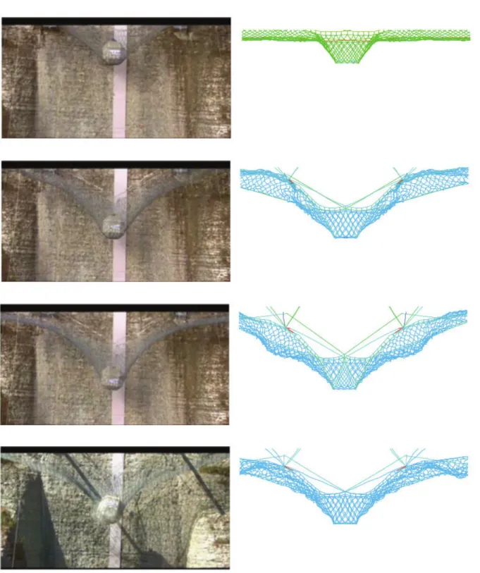
The investigation of granular flows impact on obstacles also included the physics of flows overflowing obstacles.Faug et al.(2002) experimentally investigated the dead zone formation of glass beads behind an over-passed obstacle down an inclined rough chute. The dead zone (Fig 2.3) is the zone where dead particles deposit in quasi-static condition behind the wall (Caccamo et al.,2012). Observations were taken for the length of the dead zone behind the obstacle for different slope angles and obstacles height, and was correlated with the Froude number of the flow (Fr). Froude Number is a dimensionless parameter used to indicate the influence of gravity on fluid motion (Pudasaini and

Domnik, 2009;Domnik and Pudasaini,2012;Faug et al., 2012). It measures the ratio

between the inertia force on a fluid element to the weight of that element, and is calculated as follows:

Fr = v

p g h cosα (2.1)

where v is the depth-averaged velocity of the flow, g is the gravity acceleration, h is the flow depth and α is the inclination angle of the base.

(45)

Figure 2.3:A triangular dead zone is formed upstream of a rigid wall in which moving particles overflow it. The white horizontal arrow indicates the incoming flow direction which is made of glass beads (afterCaccamo et al.,2012)

The length of the dead zone was found to increase when increasing the obstacle height, especially for low values of the inclination angles. Low values of α reduce the overflowing of the obstacle and thus increase the dead zone length. The dead zone formation will be investigated in details in the following chapters, due to its importance in characterizing the flow and impact behavior of granular flows.

Faug et al.(2011) continued investigating the dry granular flows over-topping

obsta-cles in inclined channels. First, the flow velocity and thickness were measured (in the absence of an obstacle) and dimensionlessly verified withMiDi(2004). Then, the impact force applied by dry granular flow (made of glass beads) on an overrun rigid wall was measured in the normal direction with time. The aim was to compare these results with a set of equations forming a hydrodynamic model, based on depth-averaged momentum conservation. The model takes into account the dead zone formation behind the wall and the inertial flow zone above it, and can thus predict the force applied on the wall with time (Faug et al.,2009;Chanut et al.,2010). The model’s prediction of the normal force applied on the wall, with its different components, was found to reproduce well the experimental data.

(46)

2.3 Rigid walls for debris flow hazard mitigation 17 The previous works using glass beads helped in giving an insight into the physics of dry granular flows and their impact on obstacles. However, others carried out experi-ments with real granular material (sand, gravel ..etc). Jiang and Towhata(2013) recently studied the impact behavior of dry granular flow against a rigid retaining wall using a poly-dispersed mixture of limestone gravel. Measurements of normal impact force versus time were recorded for different heights of the wall, i.e different segments forming the wall. In addition, observations of flow thickness and flow velocity were taken at the time where the total normal force on the wall reached its maximum value. These experimental data were selected for our model calibration and validation. This is because it considers elongated coarse-grained flow of angular particles rather than the simple spherical glass beads commonly used in literature. Such large-sized particles resemble a granular debris flow (coarse-grained debris) which is the aim of this thesis. In addition, the study provided detailed measurements of the time evolution of the normal impact force for different heights (different segments of the rigid wall). More details on this experiment will be given in Chapter 3.

2.3.2 Numerical modeling of granular flows impact on rigid walls

DEM has been an active method in recent years for studying the impact of granular flows on rigid walls. Faug et al.(2009) used 2D DEM simulation of spherical particles flowing in inclined channel and overflowing a rigid wall to verify their hydrodynamic model based on depth-averaged momentum conservation. In the DEM results, the normal force applied on the wall was characterized with high fluctuations due to the force chains developing in the dead zone behind the obstacle. These fluctuations are common feature of DEM modeling of impact forces. They are usually dealt with by averaging the data over small windows (Valentino et al.,2008).

Researchers also used non-spherical shape for modeling granular flows. Mollon et al.

(2012) used non-spherical particles in DEM to numerically investigate the propagation of granular masses down a slope where energy evolution was studied along with run-out mechanism. The model was validated against experimental granular flow data. Due to the limited number of particles permitted by DEM for cost considerations, the model is

(47)

Anchorage A1 A2 A3 A4 A5 Net mesh Main cable

Bottom cable (fixed to the ground) _cab1 cab2 cab3 cab4 cab5 Energy dissipator Lateral cable

W

fb

H

fb

Figure 2.4:Schematic representation of the different parts of flexible debris flow barriers

suited for small to medium sized volumes. Continuum models cannot reproduce such small sized cases involving small number of blocks as the assumption of continuous kinematic field becomes too strong.

2.4 Flexible barriers for debris flows retention

Flexible barriers are ideal for stopping debris flows due to their high deformation capacity and their water permeability (Guasti et al.,2011). In addition, in comparison with rigid walls, they distribute the impact energy over longer impact duration and thus reduce the peak impact force (Boetticher et al.,2011). Furthermore, they are advantageous for their short construction times and ease of installation in hard-to-reach terrains. Flexible barriers for debris flows mitigation are mainly composed of net elements, sliding rings, main cables, lateral cables, energy dissipators and lateral anchors (Fig. 2.4), where a good design evaluates the forces in each component. One flexible net barrier system can retain up to 2000 m3_{of debris (}_{Wendeler et al.}_,₂₀₀₈_).

(48)

2.4 Flexible barriers for debris flows retention 19

2.4.1 Flexible barriers: Rockfalls Vs. Debris flows

Flexible barriers for debris flows are similar in principle to the ones of rockfalls. However, their design is different due to the difference in their loading mechanism (Segalini et al.,

2013). For rockfalls, an energy approach is adopted for the design assuming that the kinetic energy of the boulder is instantaneously transferred to the barrier which com-pletely stops the boulder. In contrast, for debris flow flexible barriers, energy dissipation is rather gradual and thus the design approach can not be solely dependent on energy balance since the barrier loading rate can be heavily influenced by flow velocity, duration of impact .. etc. Moreover, rockfalls apply very high concentrated load at the impact point, while debris flow apply uniform load over the surface area of the barrier. As a result, different design approach better be adopted for debris flow flexible barriers as they are different in loading rate and induced stresses.

Another drawback of energy approach for debris flow flexible barriers design is that it is too conservative as it does not take into account the energy dissipated by collision due to the formation of dead zone behind the barrier (Segalini et al.,2013). In a recently published guidleinse (Volkwein,2014), this approach has been unfavored for debris flow flexible barriers design.

Instead of energy approach, the force approach can be used for the design of debris flow protection barriers (Wendeler, 2008; Segalini et al., 2013; Volkwein, 2014). It is based on the determination of the impact force applied by the flow and consequently comparing them to the barrier resistance to impact forces. The impact force is assumed to have three components: static force (due to the weight of the material), dynamic force (due to kinetic energy of the flow) and a shear force on the top cable of the barrier (in case of overflowing). More details on load estimation models on protection structures, based on the force approach, will be presented in Section 2.5.1.

(49)

2.4.2 Numerical and physical modeling of flexible barriers

The use of numerical modeling of flexible barriers enabled a more innovative design of these barriers. This is because such simulations reduce the number of required physical prototype and can test loading conditions that sometimes can not be tested on-site due to some technical and economical challenges (Volkwein,2005). In addition, numerical modeling of flexible barriers can analyze the loads in each component, and test innova-tive designs accordingly (e.g.Bertrand et al.,2012).

For the aim of modeling flexible barriers, two numerical methods have been mainly used: FEM (Cazzani et al.,2002;Castro-Fresno et al.,2008;Gentilini et al.,2012) and DEM (Nicot et al.,1999,2001;Bertrand et al.,2008,2012;Bourrier et al.,2015). Volkwein

(2005) developed an FEM-based software named "FARO" to model highly flexible bar-riers (made of ring nets) against rockfall impact. The software was calibrated against quasi-static and dynamic laboratory and field experiments and validated against data of full scale testing (Grassl,2002).

Gottardi and Govoni (2010) carried out full scale experiments of rockfall impact

on flexible barriers with kinetic energies from 500 to 5,000 kJ. Such data formed an extensive database for the calibration of numerical models of rockfall flexible barriers. Detailed results were obtained concerning the boulder breaking time, evolution of the kinetic energy, the barrier deformation and the forces applied on the anchorage and post foundations. Gentilini et al.(2012) later on used these experimental data to calibrate and validate an FEM based numerical model of rockfall flexible barriers (Fig. 2.5). The falling boulder was simulated as a set of lumped masses using the commercial software ABAQUS. Connecting cables were modeled as elasto-plastic, behaving bi-linearly.

On the other hand, DEM as a more recent numerical method, was recently deployed for modeling flexible barriers. DEM is well adapted to describe the behavior of granu-lar materials whereas FEM is mostly dedicated to modeling continuous media. Large displacements and failures between elements are easy to simulate and thus DEM is very well suited to model protection nets where important strains and failure may occur during a loading test.

(50)

2.4 Flexible barriers for debris flows retention 21

Figure 2.5:Snapshots at different time of falling boulder intercepted by a flexible barrier: FEM Numerical simulation (right) compared with photograms (left) (afterGentilini et al.,

(51)

Figure 2.6:DEM modeling of a net using remote interactions (afterBertrand et al.,2012)

The first attempt to model rockfall fences using DEM was carried out byMustoe and

Huttelmaier(1993), who used rigid connecting bodies in DEM to approximate a rockfall

fence made of truck tires. The fence was composed of a horizontal steel rod in which several hanging columnar attenuator masses composed of used tires where hanging on it.

Later,Hearn et al.(1995) andNicot et al.(2001) used DEM to develop a model for highly flexible rockfall barriers where the approach was proved to be relevant in cap-turing the dynamics of the impact of a rockfall on flexible barriers made of ring nets. Afterwards, other types of nets were efficiently modeled in DEM, including for example hexagonal meshes (Bertrand et al.,2008;Thoeni et al.,2011).

An example of the recent DEM models of flexible barriers is the work ofBertrand et al.

(2012), who modeled the net elements using remote interactions between nodes. These nodes are spherical particles placed at the intersection between the cable forming the net and the rigid clips. After detecting the contact, an elasto-plastic contact model is applied, for both loading and unloading phases. For the aim of calibrating the model, micro and meso scale experiments on single cables and punching tests of net meshes were carried out. The model was easy to calibrate as it only includes two parameters to fit: the stiffness and ultimate strength of the system. The model was then used to investigate the impact of a rigid boulder on a full-scale flexible barrier, using different loading conditions.

Discrete element modeling of the impact of granular debris flows on rigid and flexible structures

HAL Id: tel-01286617

https://tel.archives-ouvertes.fr/tel-01286617

debris flows on rigid and flexible structures

Adel Albaba

To cite this version:

THÈSE

DOCTEUR DE L’UNIVERSITÉ GRENOBLE ALPES

Adel ALBABA

Modélisation par éléments discrets de

l’impact des laves torrentielles

granulaires sur des structures rigides

et flexibles

Discrete element modeling of the

impact of granular debris flows

on rigid and flexible structures

Acknowledgement

Abstract

Résumé

Abbreviations

Contents

List of Figures

List of Tables

Chapter 1

General Introduction

Contents

1.1

Landslides and debris flows: a threat to urbanization

1.2

Research framework (MuMoLaDe Project)

1.3

Thesis objectives

1.4

Thesis structure

Chapter 2

State of the art

Contents

2.1

Introduction

2.2

Debris flows

2.2.1

Physical modeling of granular flows

2.2.2

Numerical modeling of granular flows in inclined planes

2.3

Rigid walls for debris flow hazard mitigation

2.3.1

Physical modeling of granular flows impact on rigid walls

2.3.2

Numerical modeling of granular flows impact on rigid walls

W

H

2.4

Flexible barriers for debris flows retention

2.4.1

Flexible barriers: Rockfalls Vs. Debris flows

2.4.2

Numerical and physical modeling of flexible barriers